Abstract
In recent studies, the Contrastive Language–Image Pretraining (CLIP) model has showcased remarkable versatility in downstream tasks, ranging from image captioning and question-answering reasoning to image–text similarity rating, etc. In this paper, we investigate the effectiveness of CLIP visual features in predicting perceptual image quality. CLIP is also compared with competitive large multimodal models (LMMs) for this task. In contrast to previous studies, the results show that CLIP and other LMMs do not always provide the best performance. Interestingly, our evaluation experiment reveals that combining visual features from CLIP or other LMMs with some simple distortion features can significantly enhance their performance. In some cases, the improvements are even more than 10%, while the prediction accuracy surpasses 90%.
1. Introduction
In the dynamic realm of visual content, various types of distortions are inherent in its life cycle, such as generation, processing, and delivery [1,2,3]. This has given rise to an increasing need for evaluating image quality without any reference points. In the domain of image quality assessment, particularly in the blind image quality assessment task, the emphasis has historically been on leveraging distortion features exclusively [1,2,4,5]. Recent developments have witnessed significant progress in the alignment of images with accompanying text, such as Contrastive Language–Image Pretraining (CLIP) [6]. In addition to the multimodal uses of CLIP [7,8,9,10,11], the visual features provided by CLIP have showcased remarkable versatility in diverse applications, such as captioning [12,13,14,15], object detection [16], semantic image segmentation [17], cross-modal retrieval tasks [18,19,20], etc. This wide-ranging utilization underscores the broad applicability and robust performance of CLIP and its derivatives across a spectrum of interdisciplinary challenges. Fueling this progress is the availability of massive training data used to train the image and text encoder blocks.
In this paper, our goal is to investigate how effective CLIP visual features work in image quality assessment. This is an interesting issue because, although CLIP was trained with a huge number of images and associated texts, there could be few hints for CLIP to learn which images have distortions or artifacts. So, it is not clear whether CLIP’s visual features can represent the perceptual distortions present in images.
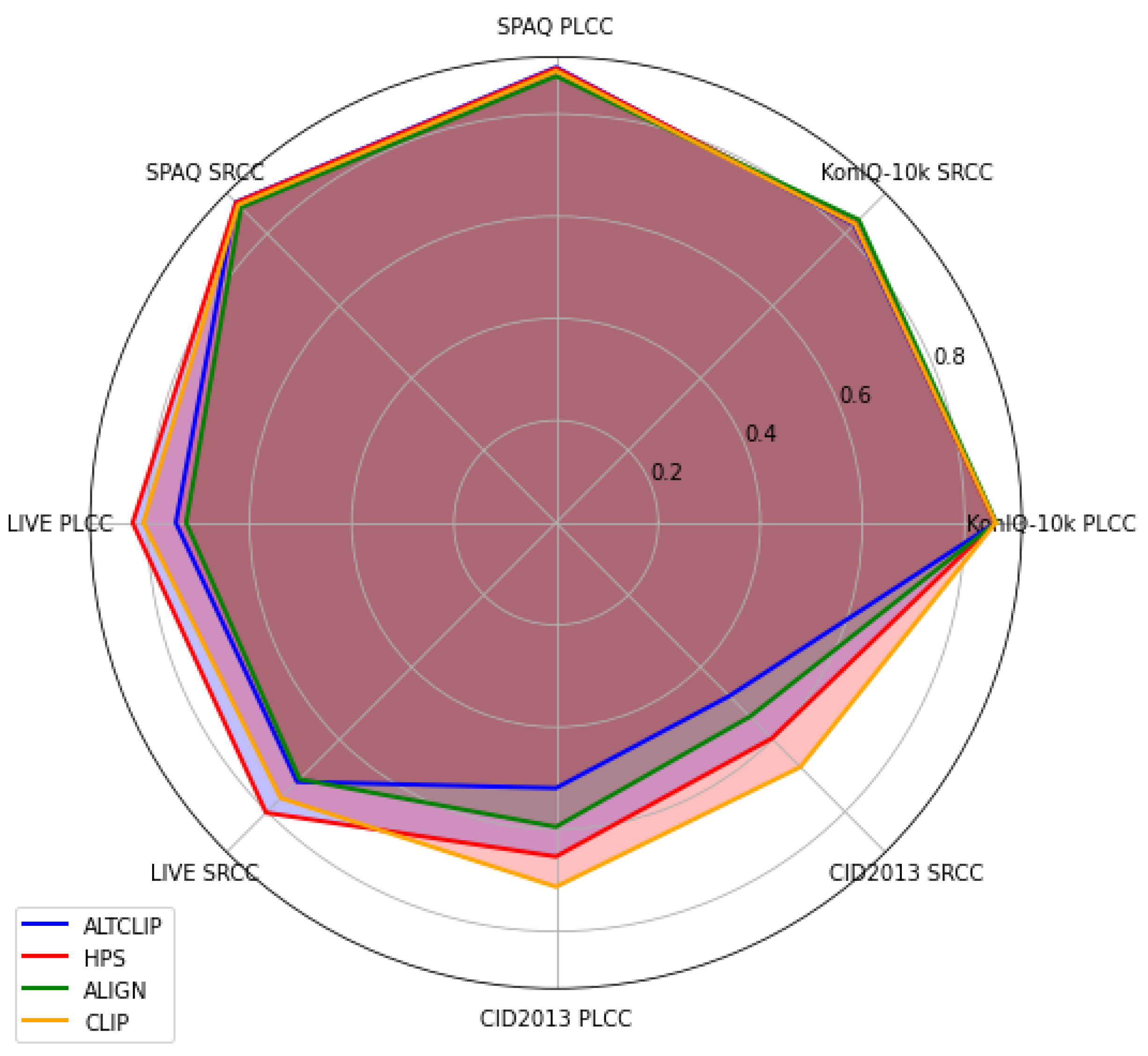
To this end, an evaluation of CLIP’s visual features for the image quality assessment (IQA) task is carried out. In particular, CLIP’s features are compared with those of related large multimodal models (LMMs), such as HPS [21], ALTCLIP [22], and ALIGN [23], and conventional features of image quality models. Through extensive experiments, it is shown that CLIP does not always provide the best performance, as seen in Figure 1. Here, the performance metrics are the Pearson Linear Correlation Coefficient (PLCC) and the Spearman Ranking Correlation Coefficient (SROCC) [24].

Figure 1.
Performance of CLIP visual features compared with other LMMs on four public natural datasets.
Remarkably, it has been observed that augmenting LMMs with simple distortion features yields a substantial enhancement in performance. This implies that service providers can efficiently extract feature vectors using various APIs and then incorporate these vectors for the purpose of quality assessment. The synergistic combination of large pretrained models with more straightforward distortion features showcases a promising avenue for assessing image qualities. To the best of our knowledge, this is the first work that comprehensively evaluates the image features of CLIP and related models for image quality assessment.
The remainder of this paper is organized as follows. Section 2 reviews and analyzes related research works, while Section 3 describes our evaluation architecture, the datasets used, and our implementation details. In Section 4, the evaluation results and the experimental findings are presented. Finally, concluding remarks are given in Section 5.
2. Related Work
This section highlights the relevant related literature in image quality assessment. Additionally, LMMs and recent research that explores using their features are presented.
2.1. Perceptual Quality Assessment
Perceptual image quality evaluation takes into account human perception factors to assess how well an image reproduces the content, colors, textures, and overall visual experience. It can be divided into three broad categories: full-reference (FR), reduced-reference (RR), and no-reference (NR) or blind image quality assessment (BIQA) [25,26]. BIQA refers to the process of evaluating the quality of a distorted image without using a reference image for comparison. It is a challenging task, as it requires the model to analyze the image content and identify potential artifacts or distortions that may affect its quality. There are various approaches to IQA, ranging from hand-crafted features [27,28,29,30] to deep learning-based methods [24,31,32,33,34,35,36].
Deep learning-based approaches have shown remarkable success in accurately evaluating image quality by leveraging the power of deep neural networks. However, a common challenge faced by deep learning methods is the availability of large-scale training datasets. In some cases, the limited availability of annotated image samples can affect the performance of IQA models [2,33]. To address this, transfer learning has been proposed as an effective solution [37,38]. Transfer learning involves pretraining a neural network on a large-scale image dataset. Subsequently, the pretrained model is fine-tuned on the IQA task using the available annotated IQA data. This approach was successfully applied in [33,34,35], where the models were pretrained on ImageNet [39] and then adapted to predict image quality scores. Additionally, the meta-learning approach in [2] can be applied to enhance the ability of IQA models to learn other distortion types prevalent in images. By employing meta-learning, the model can acquire knowledge about a wide range of distortions, improving their generalization capabilities and adaptability to diverse image datasets [2].
2.2. Large Multimodal Models
In recent times, multimodal or cross-modal learning has emerged as a thriving research area, particularly for downstream tasks like image–text similarity evaluation and image retrieval tasks. Researchers have made significant contributions by proposing robust learning models such as CLIP [6], ALIGN [23], HPS [21], ALTCLIP [22], etc., all of which aim to uncover and understand the intricate relationship between vision and language. These models often leverage advanced architectures, such as vision transformers [40], CNNs, or pretrained ResNet models [41], to effectively capture and analyze complex relationships within and between different modalities. The development of large multimodal models has been facilitated by advancements in deep learning, computational resources, and the availability of vast and diverse datasets.
The visual features of LMMs trained by text supervision can be applied for various downstream tasks. Notably, recent research conducted in [12] underscores the “unreasonable effectiveness” of the CLIP features for image captioning. They discovered that CLIP is currently one of the best visual feature extractors. Also, the research in [42] showed that CLIP can understand image aesthetics better. In their experiment, the authors trained a linear regression model using the CLIP visual features extracted from AVA datasets. Their finding shows that CLIP visual features outperform features from an ImageNet classification model. Similar to [12], the frozen CLIP features were employed in [43] for the video recognition task. It was also found that CLIP features are very effective in representing spatial features at the frame level. In the context of embodied AI tasks (e.g., robotics) [44], the use of CLIP features has been shown to be very simple but more effective than the features of ImageNet-pretrained models.
In this paper, we explore another important question: are CLIP visual features effective for perceptual image quality assessment? For this purpose, CLIP is compared with related large multimodal models, and its features are compared with those of conventional quality models.
3. Evaluation Methodology
In this section, we present a description of our evaluation architecture, LMM features, and distortion features. Also, an overview of the datasets and implementations used in our evaluation is provided.
3.1. Evaluation Architecture
Our purpose is to evaluate features from LMMs such as CLIP and related models. So, the selection and comparison of features are important for a meaningful evaluation. For this, the features were selected from various models with different degrees of complexity, as presented in Section 3.2 and Section 3.3. Also, similar to [12], as a large number of models and their feature combinations were considered in our study, we adopted a simple architecture, as depicted in Figure 2. The flow of feature processing and quality prediction is as follows. First, we extract and compare visual features from each LMM. Distorted images are passed through the image encoder block, and the visual features are extracted and input into the fully connected (FC) layer block, which serves as a regressor. Features from three typical image quality models (namely, a pretrained image quality metric, a statistical metric, and a lightweight CNN metric) are also included for comparison purposes. Second, visual features from each LMM are concatenated with the distortion features of a certain quality model, which is controlled by a switch in our architecture. Then, the vector of concatenated features is processed by the FC block to predict a quality score. The final output from the FC block is pass through a sigmoid function. The output of the sigmoid function is interpreted as the quality score between 0 and 1. During training, the objective is to minimize the Mean Squared Error (MSE) to measure the difference between the predicted score and Mean Opinion Score. The Mean Opinion Score (MOS) is a measure of perceived quality. It is an average score obtained through subjective experiments where subjects are asked to rate the images. According to the ITU-T standard P.800.1 [45], the rating typically has five levels: 5 (excellent), 4 (good), 3 (fair), 2 (poor), and 1 (bad). For image quality prediction, the MOS serves as the ground truth to judge the predicted quality score.

Figure 2.
Architecture of our evaluation study.
3.2. LMM Features
Image features are obtained by applying the respective model encoder directly to the input image in Figure 2. These model encoders are pretrained on large-scale image–text datasets such as CC-3M [46], WebText [47], Laion-400M and 5B [48,49], ALIGN training data [23], and COYO-700M [50], and they are evaluated on downstream datasets (e.g., MsCOCO [51], PascalVOC2007 [52], Flickr30k [53]) They have the capability of capturing high-level visual representations from the image data. In our study, the LMMs include CLIP [6], HPS [21], ALIGN [23], and AltCLIP [22].
3.2.1. CLIP (Contrastive Language–Image Pretraining)
CLIP [6] is a powerful model created by OpenAI for learning visual representations from natural language supervision. Trained on a vast dataset pairing images with textual descriptions, CLIP excels in tasks like visual classification and image–text retrieval [6]. CLIP is trained on WebImageText datasets [6] created by collecting 400 M image–text pairs publicly available on the Internet. It has both ViT- [40] and ResNet-based [41] backbones. For ViT-based CLIP models, CLIP ViT-/14 has 304 million parameters. CLIP ViT-B/32 and CLIP ViT-B/16 have 87.8 million and 86.2 million parameters, respectively. ResNet-based CLIP versions include RN50, RN101 (where 50 and 101 indicate the model depth), RN50x4, RN50x16, and RN50x64 (where x denotes up-scaling). CLIP-RN50x64 is the largest, with 420 million parameters, while CLIP-RN50 is the smallest, with 38.3 million parameters. CLIP-RN101 has 56.2 million parameters.
3.2.2. ALTCLIP (Alter Ego CLIP)
ALTCLIP [22] is a bilingual model designed to understand both English and Chinese. It enhances the text encoder of CLIP with XLM-R [54], a multilingual pretrained model. This means that the text encoder is a student text encoder that has learned from a teacher training stage. It uses the Conceptual Captions (CC-3M) [46] and TSL2019-5M [55] datasets as training data. The student text encoder possesses similar capabilities to the multilingual model that is used as its teacher model. Comparing both CLIP and ALTCLIP on downstream tasks like image classification using both the English and Chinese languages, CLIP outperformed ALTCLIP on the English language, while ALTCLIP outperformed CLIP on the Chinese language [22]. ALTCLIP enables cross-language understanding, allowing it to process and interpret information in both English and Chinese [22].
3.2.3. HPS (Human Preference Score)
HPS is a model designed to solve the misalignment issues (artifacts) inherent in generated images using human preferences. The study was divided into two parts: firstly, the authors [21] collected a large-scale dataset guided by human preference. Second, they designed a human preference classifier (HPC) using the collected dataset as training data [21]. The dataset is made up of 98,807 images created by 25,205 prompts of human choices. For each prompt, multiple images are provided. The user selects one image as the preferred choice, while the remaining images are considered non-preferred negatives [21]. The classifier was designed by fine-tuning CLIP ViT-L/14 with a few modifications. For both image and text encoder blocks, they used only the last 10 and 6 layers. The collected dataset was used as training data to achieve accurate semantic understanding and preference scoring. HPS was designed to guide models to generate human-preferred images.
3.2.4. ALIGN (A Large-Scale ImaGe and Noisy-Text Embedding)
ALIGN is an LMM that aligns images and noisy texts using straightforward dual encoders. It was developed as an LMM competitive with CLIP. Its image encoder backbone was designed using EfficientNet [56]. For the text encoder, the BERT base model was used. Its training data are approximately one billion noisy image alt-text pairs [23]. For image and text encoders, it has approximately 480 M and 340 M parameters, respectively. ALIGN also employs a contrastive loss to train image and text encoders. This approach facilitates the alignment of visual and textual information, making it an effective model for understanding the relationships between images and their associated noisy texts. ALIGN outperformed CLIP in downstream tasks such as image–text retrieval (Flickr30k-1K test set and MsCOCO-5K test set) and the image classification task (ImageNet) [23]. In this study, the implementation in [57], which is available in the transformer library, was used.
3.3. Distortion Features
For comparison, we also employed perceptual distortion features provided by various models that focus on the perceptual image quality. Three models were selected with increasing levels of complexity, namely, a statistical model, a lightweight CNN model, and a meta-learning model. This is important for understanding how effective LMM features are in comparison to the features that have been conventionally used to predict the quality of images.
3.3.1. Statistical Features
We used the BRISQUE (Blind/Referenceless Image Spatial Quality Evaluator) algorithm [28]. BRISQUE was developed based on the observation that the normalized luminance coefficients of natural images follow a nearly Gaussian distribution. This means that the presence of distortions can be attributed to the possible loss of naturalness. The authors designed BRISQUE [28] by using the scene statistics of locally normalized luminance coefficients to account for losses of naturalness. BRISQUE features are generated by applying the BRISQUE algorithm to each image sample. The resulting feature vector has a size of 36.
3.3.2. Lightweight CNN Features
A very simple CNN model for image quality assessment, denoted by CNNIQA [31], was employed. It is one of the earliest models developed for no-reference quality assessment. The structure is simple, with only one convolutional layer. The pooling operations include both max pooling and min pooling to pool features. For regression, 2 fully connected layers with a vector size of 800 are used. In training, both feature learning and the regression process are jointly optimized.
3.3.3. Meta-Learning Features
The state-of-the-art MetaIQA model [2] was included for our quality evaluation. This approach is based on meta-learning, which involves learning the shared meta-knowledge inherent in diverse image distortions, thereby mimicking the human visual system (HVS). The meta-learning model is based on a ResNet-18 model extensively trained on the TID2013 [58] and KADID-10k [59] datasets to learn the essential aspects of image quality distortions. The model uses bi-level gradient optimization to learn the shared meta-knowledge. To adapt to unknown data, we fine-tuned the pretrained MetaIQA model. Compared to BRISQUE and CNNIQA, the features of MetaIQA provide a much deeper representation of image quality characteristics.
3.4. Combined Features
In this study, the combined features between an LMM and a quality model were also considered. It is possible that LMMs may not have been trained with distorted images as image quality models. Therefore, augmenting LMM features with distortion features could be effective. This results in twelve (12) different combinations between the above four LMMs (CLIP, ALTCLIP, HPS, ALIGN) and the three IQA models (BRISQUE, CNNIQA, MetaIQA). As shown later in the experiments, it turns out that even the simple hand-crafted features of BRISQUE are surprisingly effective in boosting the performance of every LMM’s features.
3.5. Datasets and Implementation Details
In our evaluation, four authentically distorted IQA datasets were used. They are KonIQ-10k [60], LIVE [61], SPAQ [62], and CID2013 [63]. Through this thorough assessment, we are able to see how well the features of each LMM perform across a wide range of authentic distorted IQA datasets. Table 1 shows the characteristics of each of the selected IQA datasets. It also highlights some properties of the datasets used in our evaluation, such as the MOS range, the number of samples, and the type of subjective experiment conducted.

Table 1.
Summary of IQA datasets.
Our evaluation was implemented in PyTorch 1.10.2 for the training and testing tasks. The experimental settings, such as the learning rate, epochs, and batch size, were similar to those of MetaIQA [2]. To extract CLIP features, we used CLIP ViT-B/16 with a feature size of 512. ALTCLIP and HPS models were designed with CLIP ViT-L/14, resulting in a feature size of 768. The ALIGN model is based on EfficientNet B7 and outputs an image feature size of 640. For distortion features, the CNNIQA [31] model was adapted by resizing the default feature vector size from 800 to 512. The feature vector is passed through an FC block consisting of 3 layers. Layer 1 takes the feature vector as input, layer 2 has a size of 512, and layer 3 culminates in a single scalar value, which represents the quality score. Due to the small feature size of BRISQUE features (36), the number of FC layers was reduced to 2, with an input size of 36 and an output size of 1. The Adam optimizer [64] was used in all experiments.
4. Experiments
This section presents the experimental settings and the evaluation results. Also, the trends of different feature combination cases are discussed in detail.
4.1. Experimental Settings
In our experiment, two widely recognized metrics, SROCC and PLCC, were used to evaluate the no-reference quality assessment [1,24]. These metrics are used to quantify non-linear and linear relationships between the ground-truth MOS and the predicted scores. The scale spans from −1 to 1, where higher values signify superior predictive accuracy.
For LIVE and KonIQ-10k, we used the splitting described in [2]. For SPAQ, similar splitting to that in [62] was used. In each of the three datasets, 80% of the images were used as training samples, while the remaining 20% was used for testing. CID2013 contains 6 subsets in each set; we used four (4) subsets from each set for training and two (2) subsets for testing. For each dataset, we performed the random train–test splitting procedure 10 times and report the mean PLCC and SROCC values, along with the corresponding standard deviation (std) values. The experiment was carried out on a computer with an NVIDIA RTX 3090 GPU.
4.2. Evaluation Results
In this part, we first compare features from different LMMs and quality models. Then, the combinations of LMM features with distortion features are investigated. Also, the performance trends and behaviors of the features are discussed in detail.
The performance comparison of the features is shown in Table 2. The results reveal that MetaIQA consistently achieves the highest performance in most cases. The performance of LMM features is good but usually lower than that of MetaIQA. The only exceptions are the SRCC values of CLIP features on the CID2013 dataset and the HPS features on the LIVE dataset, which are a little higher than those of MetaIQA. Anyway, LMM features perform significantly better than the features of BRISQUE and CNNIQA. This means that large models, though trained in a general manner, can extract more distortion information than the hand-crafted or simple features of BRISQUE and CNNIQA.
Table 2.
Performance comparison using only LMM visual features on the four selected datasets. Red and blue boldfaced entries indicate the best and second best for EACH model.
The results also show that using CLIP features does not always provide the best results. More specifically, it is interesting that, when considering LMMs only, each LMM has the best performance on only one dataset (i.e., CLIP on CID2013, ALIGN on KonIQ-10k, ALTCLIP on SPAQ, and HPS on LIVE). So, no LMM can be considered the best model in this experiment.
The above results suggest that these LMMs might not have been as extensively trained with various visual distortions as MetaIQA. So, LMM features may be augmented by distortion-oriented features. For this reason, we further investigated various cases of feature combinations between an LMM and a conventional quality model. Table 3, Table 4 and Table 5 show the results of LMM features combined with the features of BRISQUE, CNNIQA, and MetaIQA, respectively.
Table 3.
Performance comparison using LMM visual features and the BRISQUE model on the four selected datasets. Red and blue boldfaced entries indicate the best and second best for each fusion type.
Table 4.
Performance comparison using LMM visual features and CNNIQA on the four selected datasets. Red and blue boldfaced entries indicate the best and second best for each fusion type.
Table 5.
Performance comparison using LMM visual features and METAIQA on the four selected datasets. Red and blue boldfaced entries indicate the best and second best for each fusion type.
In Table 3, Table 4 and Table 5, it is interesting to see that adding distortion features can significantly boost the performance of all LMMs. For instance, examining Table 3 (last row), the combination of HPS features and BRISQUE (hand-crafted) features provides the best results on three datasets (LIVE, KonIQ-10k, SPAQ), which are higher than those of MetaIQA. Meanwhile, on CID2013, the combination of CLIP and BRISQUE is the best among all LMMs and better than MetaIQA.
It should be noted that BRISQUE’s features are simply hand-crafted, and its own performance is very low, as shown in Table 2. However, it is surprisingly effective in improving the performance of LMM features. The reason could be that BRISQUE features contain low-level distortion information, which is missed by the high-level features of LMMs.
When the features of CNNIQA or MetaIQA are combined with the features of an LMM, the performance, in most cases, is further improved. This can be explained by the fact that the distortion features of CNNIQA or MetaIQA are learned features, so they are better than the hand-crafted features of BRISQUE.
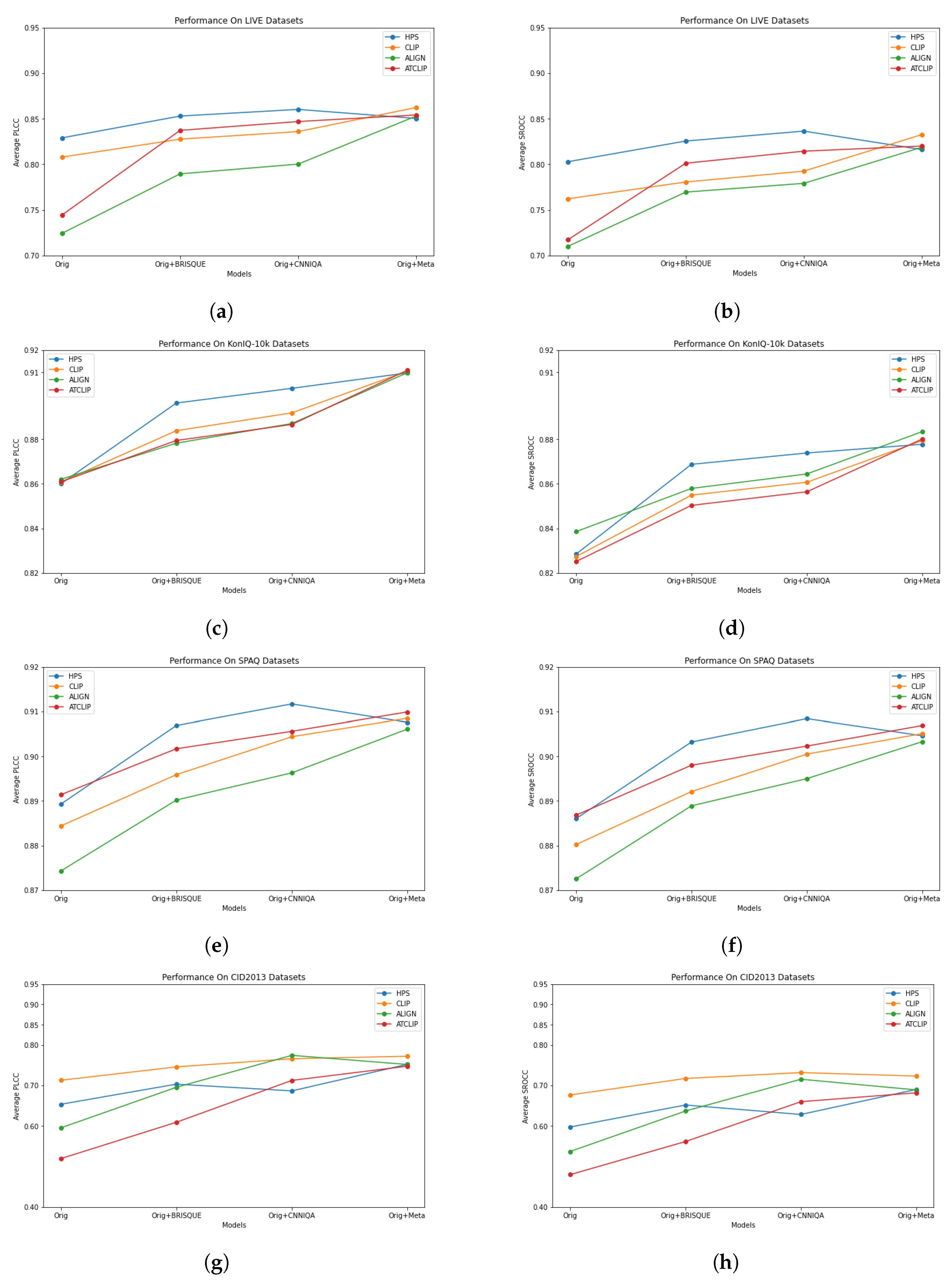
The visualization of the data in Table 2, Table 3, Table 4 and Table 5 is provided in Figure 3, where each curve shows the performance (in terms of PLCC and SROCC) for each LMM. The horizontal axis of each graph represents four cases: (1) original (denoted by “Orig”), (2) combination with BRISQUE (denoted by “Orig + BRISQUE”, (3) combination with CNNIQA (denoted by “Orig + CNNIQA”), (4) combination with MetaIQA (denoted by “Orig + Meta”). In Figure 3, the performance trends of LMM features when combined with distortion features can be more easily recognized. It is obvious that, in most cases, the gains obtained by combining features with BRISQUE, CNNIQA, or MetaIQA features increase in ascending order. This means that distortion features learned by meta-learning (i.e., MetaIQA) are richer than those by lightweight CNN learning (i.e., CNNIQA), which are, in turn, better than the simple hand-crafted features of BRISQUE. Some exception cases occur with HPS, where some combinations do not follow this trend. For example, on the LIVE dataset (Figure 3a,b), when HPS features are combined with BRISQUE features and CNNIQA features, the PLCC value is improved from 0.8290 to 0.8529 (approx. 3%) and 0.8602 (approx. 4%), respectively. But the result of the combination with MetaIQA features is just 0.8503, which is lower than that of the combination with BRISQUE. Similar behavior can be found with HPS on the SPAQ dataset. Anyway, the results of such exception cases are still better than those of using only HPS features. This phenomenon can be explained as follows. The combination of MetaIQA and HPS features may not effectively exploit the combination because both MetaIQA and HPS produce rich features, which are possibly not complementary to each other. The evaluation results suggest that LMMs only need to be combined with simple distortion features to compete with state-of-the-art quality metrics.
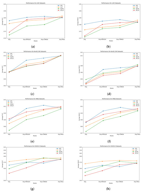
Figure 3.
Performance trends of feature combinations between LMM visual features and distortion features on the four IQA datasets. (a) PLCC on LIVE. (b) SROCC on LIVE. (c) PLCC on KonIQ-10k. (d) SROCC on KonIQ-10k. (e) PLCC on SPAQ. (f) SROCC on SPAQ. (g) PLCC on CID2013. (h) SROCC on CID2013.
From Figure 3, it can also be seen that the performance of LMM features when augmented by distortion features varies across datasets. In particular, CLIP features are only the best the on CID2013 dataset. On other datasets, the performance of HPS features is mostly higher than or comparable to that of other LMMs’ features. Notably, though the ALIGN model is the main competitor of CLIP, the performance of its features is usually lower than that of CLIP features. One exception case is the SROCC curve of ALIGN on KonIQ-10k (Figure 3d). This suggests that CLIP should be preferred to ALIGN in IQA tasks.
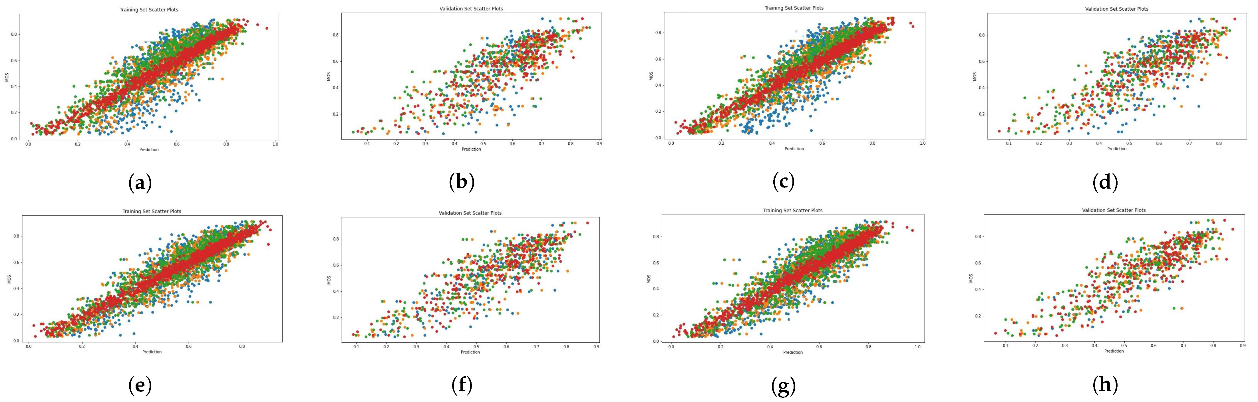
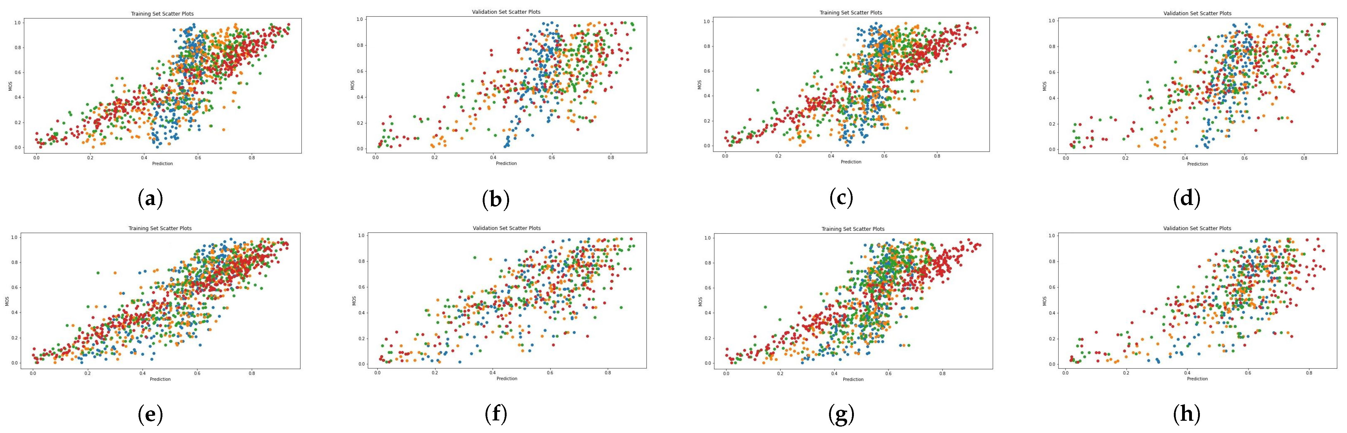
Figure 4, Figure 5, Figure 6 and Figure 7 present scatter plots, which are used to elucidate the relationship between the predicted quality score produced by our evaluation architecture and the ground-truth MOS. The scatter plots can also be used to identify anomalous patterns, outliers, or clusters that exist between the two values. As previously mentioned, our experiment involved 10 random data splits, and in this presentation, we show the results of the last split (10) and epoch 25. The scatter points marked in red, orange, and green signify the results provided by the combination of MetaIQA + LMM, BRISQUE + LMM, and CNNIQA + LMM, respectively. The results of using only LMM visual features are represented in blue color. Despite the observation of a positive relationship, it is notable that there is sparsity along the diagonal line when only LMM visual features are utilized during training. Notably, as we transition from utilizing only LMM visual features to combining them with distortion features, there is a discernible enhancement in the correlation between the predicted quality score and the ground-truth MOS values.
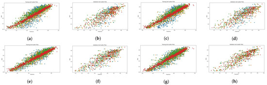
Figure 4.
Scatter diagrams showing the combination of LMM and perceptual features on the LIVE dataset. Blue: LMM visual features; orange: LMM + BRISQUE; green: LMM + CNNIQA features; red: LMM + MetaIQA. (a) ALIGN training. (b) ALIGN validation. (c) ALTCLIP training. (d) ALTCLIP validation. (e) CLIP training. (f) CLIP validation. (g) HPS training. (h) HPS validation.

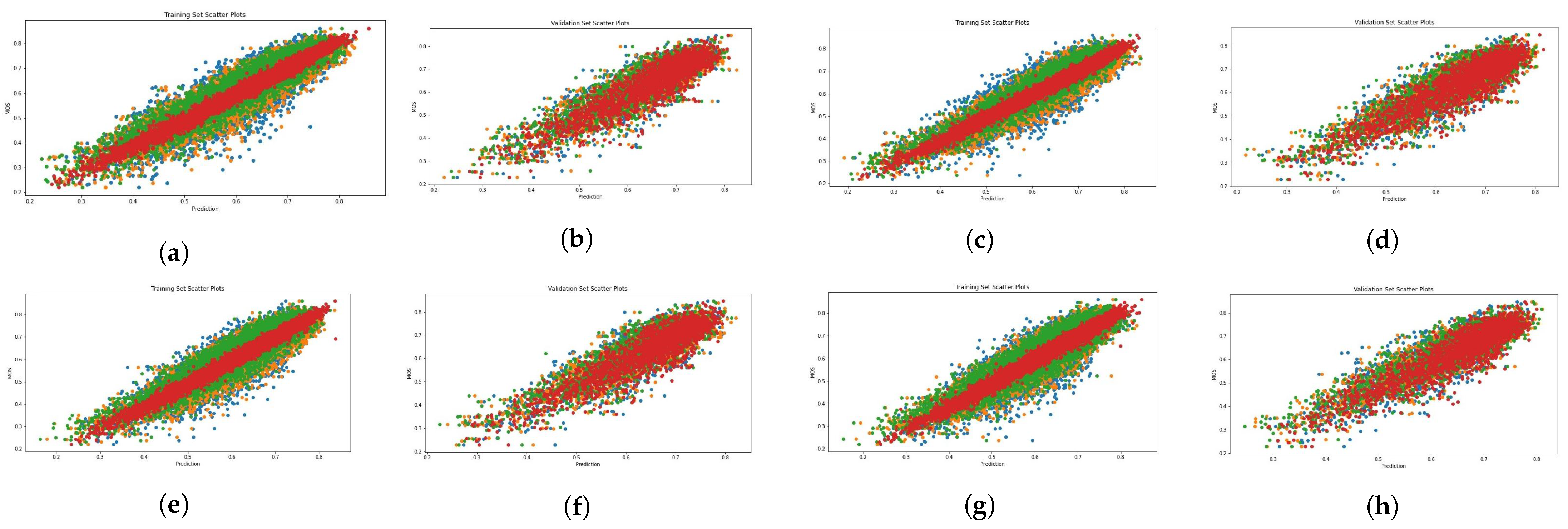
Figure 5.
Scatter diagrams showing the combination of LMM and perceptual features on the KonIQ-10k dataset. Blue: LMM visual features; orange: LMM + BRISQUE; green: LMM + CNNIQA features; red: LMM + MetaIQA. (a) ALIGN training. (b) ALIGN validation. (c) ALTCLIP training. (d) ALTCLIP validation. (e) CLIP training. (f) CLIP validation. (g) HPS training. (h) HPS validation.
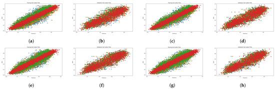
Figure 6.
Scatter diagrams showing the combination of LMM and perceptual features on the SPAQ dataset. Blue: LMM visual features; orange: LMM + BRISQUE; green: LMM + CNNIQA features; red: LMM + MetaIQA. (a) ALIGN training. (b) ALIGN validation. (c) ALTCLIP training. (d) ALTCLIP validation. (e) CLIP training. (f) CLIP validation. (g) HPS training. (h) HPS validation.
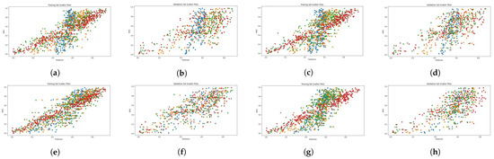
Figure 7.
Scatter diagrams showing the combination of LMM and perceptual features on the CID2013 dataset. Blue: LMM visual features; orange: LMM + BRISQUE; green: LMM + CNNIQA features; red: LMM + MetaIQA. (a) ALIGN training. (b) ALIGN validation. (c) ALTCLIP training. (d) ALTCLIP validation. (e) CLIP training. (f) CLIP validation. (g) HPS training. (h) HPS validation.
5. Conclusions
Recently, the Contrastive Language–Image Pretraining (CLIP) model and related large multimodal models (LMMs) have been introduced as key achievements in the deep learning era. In this study, we investigated the use of the visual features of CLIP and related LMMs for perceptual image quality assessment. Based on the obtained results and above discussions, the key findings from this evaluation study can be summarized as follows:
- The features of LMMs still cannot be as effective as those of state-of-the-art IQA models. This could be because the training data of these models do not specifically include distorted images with quality scores as labels. However, the performance of LMM features is much better than that of hand-crafted features or that of lightweight CNN.
- CLIP features have the best results on only one dataset. In fact, the performance of different LMMs varies widely, depending on the given dataset and the feature combination.
- The features of ALIGN, which is the main competitor of CLIP, usually are not as effective as the features of CLIP and its variants in image quality assessment. In addition, the cases involving features from HPS demonstrate exceptional performance, especially on large IQA datasets.
- An important finding is that distortion features can be combined with LMM features to significantly boost performance. Even the very basic distortion features of BRISQUE are useful in improving the performance of LMM features.
The above findings suggest that, in practice, developers may just extract LMM features and simple distortion features using some existing APIs, without having to build new and complex models for IQA. The synergistic combination of LMM visual features with traditional distortion features showcases a promising and efficient approach to image quality assessment. In future work, we will extend our investigation to the quality assessment of video contents.
Author Contributions
Conceptualization, C.O., J.F. and T.C.T.; methodology, C.O., J.F. and T.C.T.; software, C.O. and J.F.; validation, C.O. and T.C.T.; investigation, C.O., J.F., and T.C.T.; resources, C.O. and J.F.; data curation, C.O. and J.F.; writing—original draft preparation, C.O., J.F. and T.C.T.; visualization, C.O.; supervision, T.C.T.; project administration, T.C.T.; funding acquisition, T.C.T. All authors have read and agreed to the published version of the manuscript.
Funding
This research was supported in part by JSPS KAKENHI, Grant No. 22K12299.
Data Availability Statement
Derived data supporting the findings of this study are available from the corresponding author on request.
Conflicts of Interest
The authors declare no conflicts of interest.
References
- Nguyen, D.; Tran, H.; Thang, T.C. An ensemble learning-based no reference qoe model for user generated contents. In Proceedings of the 2021 IEEE International Conference on Multimedia & Expo Workshops (ICMEW), Shenzhen, China, 5–9 July 2021; IEEE: Piscataway, NJ, USA, 2021; pp. 1–6. [Google Scholar]
- Zhu, H.; Li, L.; Wu, J.; Dong, W.; Shi, G. MetaIQA: Deep meta-learning for no-reference image quality assessment. In Proceedings of the IEEE/CVF Conference on Computer Vision and Pattern Recognition, Seattle, WA, USA, 13–19 June 2020; pp. 14143–14152. [Google Scholar]
- Nguyen, H.N.; Vu, T.; Le, H.T.; Ngoc, N.P.; Thang, T.C. Smooth quality adaptation method for VBR video streaming over HTTP. In Proceedings of the 2015 International Conference on Communications, Management and Telecommunications (ComManTel), DaNang, Vietnam, 28–30 December 2015; IEEE: Piscataway, NJ, USA, 2015; pp. 184–188. [Google Scholar]
- Tran, H.T.; Nguyen, D.; Thang, T.C. An open software for bitstream-based quality prediction in adaptive video streaming. In Proceedings of the 11th ACM Multimedia Systems Conference, Istanbul, Turkey, 8–11 June 2020; pp. 225–230. [Google Scholar]
- Tran, H.T.; Ngoc, N.P.; Hoßfeld, T.; Seufert, M.; Thang, T.C. Cumulative quality modeling for HTTP adaptive streaming. ACM Trans. Multimed. Comput. Commun. Appl. (TOMM) 2021, 17, 1–24. [Google Scholar] [CrossRef]
- Radford, A.; Kim, J.W.; Hallacy, C.; Ramesh, A.; Goh, G.; Agarwal, S.; Sastry, G.; Askell, A.; Mishkin, P.; Clark, J.; et al. Learning transferable visual models from natural language supervision. In Proceedings of the International Conference on Machine Learning, Virtual, 18–24 July 2021; pp. 8748–8763. [Google Scholar]
- Alpay, T.; Magg, S.; Broze, P.; Speck, D. Multimodal video retrieval with CLIP: A user study. Inf. Retr. J. 2023, 26, 6. [Google Scholar] [CrossRef]
- Wu, H.H.; Seetharaman, P.; Kumar, K.; Bello, J.P. Wav2clip: Learning robust audio representations from clip. In Proceedings of the ICASSP 2022–2022 IEEE International Conference on Acoustics, Speech and Signal Processing (ICASSP), Singapore, 23–27 May 2022; IEEE: Piscataway, NJ, USA, 2022; pp. 4563–4567. [Google Scholar]
- Flaherty, J.; Onuoha, C.; Paik, I.; Thang, T.C. AI to Judge AI-Generated Images: Both Semantics and Perception Matter. In Proceedings of the 2023 IEEE 13th International Conference on Consumer Electronics-Berlin (ICCE-Berlin), Berlin, Germany, 3–5 September 2023; IEEE: Piscataway, NJ, USA, 2023; pp. 51–52. [Google Scholar]
- Lan, Y.; Li, X.; Liu, X.; Li, Y.; Qin, W.; Qian, W. Improving Zero-shot Visual Question Answering via Large Language Models with Reasoning Question Prompts. In Proceedings of the 31st ACM International Conference on Multimedia, Ottawa, ON, Canada, 29 October–3 November 2023; pp. 4389–4400. [Google Scholar]
- Zhao, M.; Li, B.; Wang, J.; Li, W.; Zhou, W.; Zhang, L.; Xuyang, S.; Yu, Z.; Yu, X.; Li, G.; et al. Towards video text visual question answering: Benchmark and baseline. Adv. Neural Inf. Process. Syst. 2022, 35, 35549–35562. [Google Scholar]
- Barraco, M.; Cornia, M.; Cascianelli, S.; Baraldi, L.; Cucchiara, R. The unreasonable effectiveness of CLIP features for image captioning: An experimental analysis. In Proceedings of the IEEE/CVF Conference on Computer Vision and Pattern Recognition, New Orleans, LA, USA, 18–24 June 2022; pp. 4662–4670. [Google Scholar]
- Tang, M.; Wang, Z.; Liu, Z.; Rao, F.; Li, D.; Li, X. Clip4caption: Clip for video caption. In Proceedings of the 29th ACM International Conference on Multimedia, Virtual Event, China, 20–24 October 2021; pp. 4858–4862. [Google Scholar]
- Shen, S.; Li, L.H.; Tan, H.; Bansal, M.; Rohrbach, A.; Chang, K.W.; Yao, Z.; Keutzer, K. How much can clip benefit vision-and-language tasks? arXiv 2021, arXiv:2107.06383. [Google Scholar]
- Mokady, R.; Hertz, A.; Bermano, A.H. Clipcap: Clip prefix for image captioning. arXiv 2021, arXiv:2111.09734. [Google Scholar]
- He, Y.; Huang, Z.; Liu, Q.; Wang, Y. Incremental Object Detection with CLIP. arXiv 2023, arXiv:2310.08815. [Google Scholar]
- Wang, Z.; Lu, Y.; Li, Q.; Tao, X.; Guo, Y.; Gong, M.; Liu, T. Cris: Clip-driven referring image segmentation. In Proceedings of the IEEE/CVF Conference on Computer Vision and Pattern Recognition, New Orleans, LA, USA, 18–24 June 2022; pp. 11686–11695. [Google Scholar]
- Wang, J.; Wang, H.; Deng, J.; Wu, W.; Zhang, D. Efficientclip: Efficient cross-modal pre-training by ensemble confident learning and language modeling. arXiv 2023, arXiv:2109.04699. [Google Scholar]
- Huang, S.; Gong, B.; Pan, Y.; Jiang, J.; Lv, Y.; Li, Y.; Wang, D. VoP: Text-Video Co-operative Prompt Tuning for Cross-Modal Retrieval. In Proceedings of the IEEE/CVF Conference on Computer Vision and Pattern Recognition, Vancouver, BC, Canada, 17–24 June 2023; pp. 6565–6574. [Google Scholar]
- Xia, X.; Dong, G.; Li, F.; Zhu, L.; Ying, X. When CLIP meets cross-modal hashing retrieval: A new strong baseline. Inf. Fusion 2023, 100, 101968. [Google Scholar] [CrossRef]
- Wu, X.; Sun, K.; Zhu, F.; Zhao, R.; Li, H. Better aligning text-to-image models with human preference. arXiv 2023, arXiv:2303.14420. [Google Scholar]
- Chen, Z.; Liu, G.; Zhang, B.W.; Ye, F.; Yang, Q.; Wu, L. Altclip: Altering the language encoder in clip for extended language capabilities. arXiv 2022, arXiv:2211.06679. [Google Scholar]
- Jia, C.; Yang, Y.; Xia, Y.; Chen, Y.T.; Parekh, Z.; Pham, H.; Le, Q.; Sung, Y.H.; Li, Z.; Duerig, T. Scaling up visual and vision-language representation learning with noisy text supervision. In Proceedings of the International Conference on Machine Learning, Virtual, 18–24 July 2021; pp. 4904–4916. [Google Scholar]
- Bosse, S.; Maniry, D.; Müller, K.R.; Wiegand, T.; Samek, W. Deep neural networks for no-reference and full-reference image quality assessment. IEEE Trans. Image Process. 2017, 27, 206–219. [Google Scholar] [CrossRef]
- He, L.; Gao, F.; Hou, W.; Hao, L. Objective image quality assessment: A survey. Int. J. Comput. Math. 2014, 91, 2374–2388. [Google Scholar] [CrossRef]
- Akhtar, Z.; Falk, T.H. Audio-visual multimedia quality assessment: A comprehensive survey. IEEE Access 2017, 5, 21090–21117. [Google Scholar] [CrossRef]
- Gao, X.; Gao, F.; Tao, D.; Li, X. Universal blind image quality assessment metrics via natural scene statistics and multiple kernel learning. IEEE Trans. Neural Netw. Learn. Syst. 2013, 24, 2013–2026. [Google Scholar]
- Mittal, A.; Moorthy, A.K.; Bovik, A.C. No-reference image quality assessment in the spatial domain. IEEE Trans. Image Process. 2012, 21, 4695–4708. [Google Scholar] [CrossRef]
- Moorthy, A.K.; Bovik, A.C. A two-step framework for constructing blind image quality indices. IEEE Signal Process. Lett. 2010, 17, 513–516. [Google Scholar] [CrossRef]
- Saad, M.A.; Bovik, A.C.; Charrier, C. Blind image quality assessment: A natural scene statistics approach in the DCT domain. IEEE Trans. Image Process. 2012, 21, 3339–3352. [Google Scholar] [CrossRef] [PubMed]
- Kang, L.; Ye, P.; Li, Y.; Doermann, D. Convolutional neural networks for no-reference image quality assessment. In Proceedings of the IEEE Conference on Computer Vision and Pattern Recognition, Columbus, OH, USA, 23–28 June 2014; pp. 1733–1740. [Google Scholar]
- Zhang, W.; Ma, K.; Yan, J.; Deng, D.; Wang, Z. Blind image quality assessment using a deep bilinear convolutional neural network. IEEE Trans. Circuits Syst. Video Technol. 2018, 30, 36–47. [Google Scholar] [CrossRef]
- Bianco, S.; Celona, L.; Napoletano, P.; Schettini, R. On the use of deep learning for blind image quality assessment. Signal Image Video Process. 2018, 12, 355–362. [Google Scholar] [CrossRef]
- Zeng, H.; Zhang, L.; Bovik, A.C. A probabilistic quality representation approach to deep blind image quality prediction. arXiv 2017, arXiv:1708.08190. [Google Scholar]
- Talebi, H.; Milanfar, P. NIMA: Neural image assessment. IEEE Trans. Image Process. 2018, 27, 3998–4011. [Google Scholar] [CrossRef]
- Ma, K.; Liu, W.; Zhang, K.; Duanmu, Z.; Wang, Z.; Zuo, W. End-to-end blind image quality assessment using deep neural networks. IEEE Trans. Image Process. 2017, 27, 1202–1213. [Google Scholar] [CrossRef]
- Zhuang, F.; Qi, Z.; Duan, K.; Xi, D.; Zhu, Y.; Zhu, H.; Xiong, H.; He, Q. A comprehensive survey on transfer learning. Proc. IEEE 2020, 109, 43–76. [Google Scholar] [CrossRef]
- Ribani, R.; Marengoni, M. A survey of transfer learning for convolutional neural networks. In Proceedings of the 2019 32nd SIBGRAPI Conference on Graphics, Patterns and Images Tutorials (SIBGRAPI-T), Rio de Janeiro, Brazil, 28–31 October 2019; IEEE: Piscataway, NJ, USA, 2019; pp. 47–57. [Google Scholar]
- Deng, J.; Dong, W.; Socher, R.; Li, L.J.; Li, K.; Fei-Fei, L. ImageNet: A large-scale hierarchical image database. In Proceedings of the 2009 IEEE Conference on Computer Vision and Pattern Recognition, Miami, FL, USA, 20–25 June 2009; pp. 248–255. [Google Scholar] [CrossRef]
- Dosovitskiy, A.; Beyer, L.; Kolesnikov, A.; Weissenborn, D.; Zhai, X.; Unterthiner, T.; Dehghani, M.; Minderer, M.; Heigold, G.; Gelly, S.; et al. An image is worth 16x16 words: Transformers for image recognition at scale. arXiv 2020, arXiv:2010.11929. [Google Scholar]
- He, K.; Zhang, X.; Ren, S.; Sun, J. Deep residual learning for image recognition. In Proceedings of the IEEE Conference on Computer Vision and Pattern Recognition, Las Vegas, NV, USA, 27–30 June 2016; pp. 770–778. [Google Scholar]
- Hentschel, S.; Kobs, K.; Hotho, A. CLIP knows image aesthetics. Front. Artif. Intell. 2022, 5, 976235. [Google Scholar] [CrossRef] [PubMed]
- Lin, Z.; Geng, S.; Zhang, R.; Gao, P.; de Melo, G.; Wang, X.; Dai, J.; Qiao, Y.; Li, H. Frozen clip models are efficient video learners. In Proceedings of the European Conference on Computer Vision, Tel Aviv, Israel, 23–27 October 2022; Springer: Cham, Switzerland, 2022; pp. 388–404. [Google Scholar]
- Khandelwal, A.; Weihs, L.; Mottaghi, R.; Kembhavi, A. Simple but effective: Clip embeddings for embodied ai. In Proceedings of the IEEE/CVF Conference on Computer Vision and Pattern Recognition, New Orleans, LA, USA, 18–24 June 2022; pp. 14829–14838. [Google Scholar]
- RECOMMENDATION P.800.1; Mean Opinion Score (MOS) Terminology. ITU-T: Geneva, Switzerland, 2016.
- Sharma, P.; Ding, N.; Goodman, S.; Soricut, R. Conceptual captions: A cleaned, hypernymed, image alt-text dataset for automatic image captioning. In Proceedings of the 56th Annual Meeting of the Association for Computational Linguistics (Volume 1: Long Papers), Melbourne, Australia, 15–20 July 2018; pp. 2556–2565. [Google Scholar]
- Radford, A.; Wu, J.; Child, R.; Luan, D.; Amodei, D.; Sutskever, I. Language models are unsupervised multitask learners. OpenAI Blog 2019, 1, 9. [Google Scholar]
- Schuhmann, C.; Vencu, R.; Beaumont, R.; Kaczmarczyk, R.; Mullis, C.; Katta, A.; Coombes, T.; Jitsev, J.; Komatsuzaki, A. Laion-400m: Open dataset of clip-filtered 400 million image-text pairs. arXiv 2021, arXiv:2111.02114. [Google Scholar]
- Schuhmann, C.; Beaumont, R.; Vencu, R.; Gordon, C.; Wightman, R.; Cherti, M.; Coombes, T.; Katta, A.; Mullis, C.; Wortsman, M.; et al. Laion-5b: An open large-scale dataset for training next generation image-text models. Adv. Neural Inf. Process. Syst. 2022, 35, 25278–25294. [Google Scholar]
- Byeon, M.; Park, B.; Kim, H.; Lee, S.; Baek, W.; Kim, S. COYO-700M: Image-Text Pair Dataset. 2022. Available online: https://github.com/kakaobrain/coyo-dataset (accessed on 20 November 2023).
- Lin, T.Y.; Maire, M.; Belongie, S.; Hays, J.; Perona, P.; Ramanan, D.; Dollár, P.; Zitnick, C.L. Microsoft coco: Common objects in context. In Proceedings of the Computer Vision–ECCV 2014: 13th European Conference, Zurich, Switzerland, 6–12 September 2014; Proceedings, Part V 13. Springer: Cham, Switzerland, 2014; pp. 740–755. [Google Scholar]
- Everingham, M.; Van Gool, L.; Williams, C.K.I.; Winn, J.; Zisserman, A. The PASCAL Visual Object Classes Challenge 2007 (VOC2007) Results. Available online: http://www.pascal-network.org/challenges/VOC/voc2007/workshop/index.html (accessed on 20 November 2023).
- Young, P.; Lai, A.; Hodosh, M.; Hockenmaier, J. From image descriptions to visual denotations: New similarity metrics for semantic inference over event descriptions. Trans. Assoc. Comput. Linguist. 2014, 2, 67–78. [Google Scholar] [CrossRef]
- Conneau, A.; Khandelwal, K.; Goyal, N.; Chaudhary, V.; Wenzek, G.; Guzmán, F.; Grave, E.; Ott, M.; Zettlemoyer, L.; Stoyanov, V. Unsupervised cross-lingual representation learning at scale. arXiv 2019, arXiv:1911.02116. [Google Scholar]
- Xu, B. Nlp chinese corpus: Large scale chinese corpus for nlp. Zenodo 2019. [Google Scholar]
- Tan, M.; Le, Q. Efficientnet: Rethinking model scaling for convolutional neural networks. In Proceedings of the International Conference on Machine Learning, 2019, Long Beach, CA, USA, 9–15 June 2019; 2019; pp. 6105–6114. [Google Scholar]
- Yoon, B.; Lee, Y.; Baek, W. COYO-ALIGN. 2022. Available online: https://github.com/kakaobrain/coyo-align (accessed on 13 August 2023).
- Ponomarenko, N.; Ieremeiev, O.; Lukin, V.; Egiazarian, K.; Jin, L.; Astola, J.; Vozel, B.; Chehdi, K.; Carli, M.; Battisti, F.; et al. Color image database TID2013: Peculiarities and preliminary results. In Proceedings of the European Workshop on Visual Information Processing (EUVIP), Paris, France, 10–12 June 2013; IEEE: Piscataway, NJ, USA, 2013; pp. 106–111. [Google Scholar]
- Lin, H.; Hosu, V.; Saupe, D. KADID-10k: A Large-scale Artificially Distorted IQA Database. In Proceedings of the 2019 Tenth International Conference on Quality of Multimedia Experience (QoMEX), Berlin, Germany, 5–7 June 2019; IEEE: Piscataway, NJ, USA, 2019; pp. 1–3. [Google Scholar]
- Hosu, V.; Lin, H.; Sziranyi, T.; Saupe, D. KonIQ-10k: An ecologically valid database for deep learning of blind image quality assessment. IEEE Trans. Image Process. 2020, 29, 4041–4056. [Google Scholar] [CrossRef] [PubMed]
- Ghadiyaram, D.; Bovik, A.C. Massive online crowdsourced study of subjective and objective picture quality. IEEE Trans. Image Process. 2015, 25, 372–387. [Google Scholar] [CrossRef] [PubMed]
- Fang, Y.; Zhu, H.; Zeng, Y.; Ma, K.; Wang, Z. Perceptual quality assessment of smartphone photography. In Proceedings of the IEEE/CVF Conference on Computer Vision and Pattern Recognition, Seattle, WA, USA, 13–19 June 2020; pp. 3677–3686. [Google Scholar]
- Virtanen, T.; Nuutinen, M.; Vaahteranoksa, M.; Oittinen, P.; Häkkinen, J. CID2013: A database for evaluating no-reference image quality assessment algorithms. IEEE Trans. Image Process. 2014, 24, 390–402. [Google Scholar] [CrossRef]
- Kingma, D.P.; Ba, J. Adam: A method for stochastic optimization. arXiv 2014, arXiv:1412.6980. [Google Scholar]


Disclaimer/Publisher’s Note: The statements, opinions and data contained in all publications are solely those of the individual author(s) and contributor(s) and not of MDPI and/or the editor(s). MDPI and/or the editor(s) disclaim responsibility for any injury to people or property resulting from any ideas, methods, instructions or products referred to in the content. |
© 2024 by the authors. Licensee MDPI, Basel, Switzerland. This article is an open access article distributed under the terms and conditions of the Creative Commons Attribution (CC BY) license (https://creativecommons.org/licenses/by/4.0/).