Hierarchical Classification for Large-Scale Learning

Abstract

Deep neural networks (DNNs) have drawn much attention due to their success in various vision tasks. Current DNNs are used on data with a relatively small number of classes (e.g., 1000 or less) and employ a fully connected layer for classification, which allocates one neuron for each class and thus, per-example, the classification scales as $O\left(K\right)$ with the number of classes K. This approach is computationally intensive for many real-life applications where the number of classes is very large (e.g., tens of thousands of classes). To address this problem, our paper introduces a hierarchical approach for classification with a large number of classes that scales as $O\left(\sqrt{K}\right)$ and could be extended to $O\left(\log K\right)$ with a deeper hierarchy. The method, called Hierarchical PPCA, uses a self-supervised pretrained feature extractor to obtain meaningful features and trains Probabilistic PCA models on the extracted features for each class separately, making it easy to add classes without retraining the whole model. The Mahalanobis distance is used to obtain the classification result. To speed-up classification, the proposed Hierarchical PPCA framework clusters the image class models, represented as Gaussians, into a smaller number of super-classes using a modified k-means clustering algorithm. The classification speed increase is obtained by Hierarchical PPCA assigning a sample to a small number of the most likely super-classes and restricting the image classification to the image classes corresponding to these super-classes. The fact that the model is trained on each class separately makes it applicable to training on very large datasets such as the whole ImageNet with more than 10,000 classes. Experiments on three standard datasets (ImageNet-100, ImageNet-1k,and ImageNet-10k) indicate that the hierarchical classifier can achieve a superior accuracy with up to a 16-fold speed increase compared to a standard fully connected classifier.

1. Introduction

Deep learning models emerged to surpass human performance on multiple vision tasks [1,2]. Artificial neural networks employ layers of biologically inspired neurons that are learned by different variants of gradient descent [3,4]. Despite their success, deep learning models are regarded as a black box because the process in which the individual neurons generate outputs is not interpretable [5,6]. Moreover, deep learning classifiers do not construct a hierarchy of concepts explicitly and use a fully connected layer for classification, which predicts a score for each of the existing classes, thus scaling as $O\left(K\right)$ with the number K of classes. While this approach is reasonable for current datasets with up to $K=1000$ classes, it becomes cumbersome and computationally expensive when the number of classes increases to tens of thousands of classes or more.

On the other hand, humans can establish hierarchical semantic relations between categories, which are learned by much fewer samples than deep learning models. In this respect, [7] stated that the human cognitive architecture is composed of substructures for hierarchical processing. Using this hierarchical representation, humans are capable of easily recognizing millions of classes of objects and can add new classes with just a few examples and no retraining.

Models like symbolic systems attempted to simulate the high-level reasoning processes of humans (classification logic and temporal logic). For example, ref. [8] has proposed that rule-based hierarchical classification is biologically inherited by humans or other non-human mammals like baboons. Furthermore, ref. [9] proposed a framework known as neural symbolic system artificial neural networks (ANNs). It provides the framework for parallel computation and robust learning while logic units provide interpretability. However, most symbolic systems often require problem-specific manual tuning features [10], and are not able to learn features from raw input data [11].

In this context, the research question that this paper tries to address is the following:

Can image classification models be organized hierarchically to speed-up per example classification from $O\left(K\right)$ to $O\left(\sqrt{K}\right)$ or faster, where K is the number of classes?

To address this question, we introduce a hierarchical framework for object classification called Hierarchical PPCA, which is inspired by our understanding of human hierarchical cognition. In this work, a two-level taxonomy is used to model the semantic hierarchy of image classes, but more levels could also be used if desired. Image classes are conceptualized as Gaussian distributions with Probabilistic Principal Component Analysis (PPCA) models. Instead of standard neurons, the classifier is constructed using PPCA neurons. We assume that image classes with similar semantic information will cluster together, each semantic cluster being characterized by its centroid (a Gaussian), which we refer to as a super-class. For this purpose, we introduce a modified k-means clustering algorithm to explore underlying semantic relations between image classes and build the class hierarchy. In the classification stage, an image of a cat will first be assigned to a super-class like ‘animal’ and then classified among the image classes associated with the ‘animal’ super-class. This hierarchical scheme facilitates sparse neuron firing and requires considerably less computation resources than the traditional flat structure. If the dataset contains K classes, the hierarchical model can classify images in $O\left(\sqrt{K}\right)$ time instead of $O\left(K\right)$ as in standard classification. Experiments have shown that Hierarchical PPCA can applied to large-scale datasets with superior accuracy and efficiency.

The main contributions of the proposed Hierarchical PPCA method are:

• It introduces a hierarchical classification model for learning from datasets with a large number of classes, without hierarchical annotation. The image classes are modeled as Gaussian distributions based on Probabilistic PCA (PPCA). The model reduces the per-observation classification time for K classes from $O\left(K\right)$ to $O\left(\sqrt{K}\right)$, and potentially to $O\left(\log K\right)$ when using more hierarchy levels.
• It presents an efficient training procedure based on a generalization of k-means clustering that clusters image classes instead of features. This design can handle unbalanced data where the number of observations in each class differs widely.
• It conducts experiments on large-scale datasets that show that indeed the hierarchical approach can speed-up classification without any loss in accuracy.

The paper is organized as follows. Section 2 presents a review of the literature on hierarchical clustering and hierarchical models for vision. Section 3 presents an overview of our Probabilistic PCA, which is the foundation on which the proposed Hierarchical PPCA is built. Section 4 presents the proposed Hierarchical PPCA method that clusters the PPCA Gaussians into a smaller number of super-classes and uses the super-classes to speed-up classification for a given example. Section 5 presents experiments on three datasets with 100, 1000 and 10,450 classes to evaluate the increase in speed and accuracy of the proposed method. Finally, Section 6 finishes with conclusions and a discussion on future work.

2. Related Work

The related work can be divided into hierarchical clustering work and hierarchical models in computer vision.

2.1. Hierarchical Clustering

Hierarchical clustering (HCA) is an unsupervised method of cluster analysis that seeks to build a hierarchy of clusters [12]. Much early work on hierarchical clustering was in the field of biological taxonomy.

Agglomerative clustering [13] is a dominant HCA method that works in a bottom-up manner. The main idea behind agglomerative clustering is to find the closest pair of clusters and merge them together. This process is repeated until all the data points are merged into a single cluster. The distance between two clusters is usually measured using a distance metric, such as the Euclidean distance or cosine similarity. The most common method for merging two clusters is the single linkage method, which merges the two clusters that are closest to each other. One of the main advantages of agglomerative clustering is its simplicity and ease of implementation. It is also useful for identifying hierarchical structures within the data, as it produces a dendrogram that shows how the clusters are nested within each other. This can be useful for visualizing the relationships between different groups of data. However, agglomerative clustering can be computationally expensive and may not scale well to large datasets. Agglomerative clustering for n data points has a time complexity of $O\left(n^3\right)$ and requires $O\left(n^2\right)$ memory, which makes it unpractical for even medium size datasets.

Another variant of HCA is divisive clustering [5], which works in a top-down manner. The algorithm starts at the top with all observations in one cluster. The cluster is split using a flat clustering algorithm. This procedure is applied recursively until each observation is in its own singleton cluster. Top-down clustering is conceptually more complex than bottom-up clustering. Divisive clustering with an exhaustive search is $O\left(2^n\right)$, but it is common to use faster heuristics to choose the splits, such as k-means, which is $O\left(n\right)$. However, divisive clustering is more efficient if it does not generate a complete hierarchy all the way down to individual observations. Hierarchical clustering has the distinct advantage that any valid measure of distance can be used. However, due to its limitations in time complexity, it might not be applicable to large-scale datasets.

The proposed clustering method is a variant of the k-means algorithm, adapted to cluster Gaussians instead of observations. In that respect it differs from the standard k-means in that it uses a different distance measure between observations (the Bhattacharyya distance instead of the Euclidean distance), a different distance measure between observations and the cluster models (the KL-divergence instead of the Mahalanobis distance), and an explicit analytic formula for the cluster centroid (that minimizes the average KL divergence to the cluster elements).

2.2. Hierarchical Models for Vision Tasks

Some efforts aim to explore the hierarchical semantic nature for vision tasks [14].

A manually defined hierarchy of concepts is used in [15] for class recognition. It combines image classifiers from different hierarchical levels into a single classifier to improve classification accuracy. However, since the hierarchies are defined by hand, they might not be optimal for computation considerations and could become impractical when dealing with tens of thousands of classes.

Word semantics of image labels are used in [16] to integrate prior information about inter-class relationships into visual concept learning. They built a semantic hierarchy of discriminative classifiers for object detection. The hierarchy used is inherited from the word hierarchy, which might not be computationally optimal.

A hierarchical framework capable of learning visual abstraction from a small number of images is proposed in [17]. The hierarchy is learned from the confusion matrix of a flat classifier on the learned classes. However, this hierarchy is not used to speed up classification, but is evaluated for the quality of its nodes (called concepts) using human annotators.

Ref. [18] propose a method that benefits from CNNs and hierarchical prior knowledge when the training set is small. They have shown that the prior label tree can be used to transfer knowledge between classes and boost performance when insufficient training examples are available.

Ref. [19] propose a model that learns the visual similarities between various clothing categories and predicts a tree of categories. They propose a novel object detection method that can handle newer categories without the need for obtaining new labeled data and retraining the network.

This work relies heavily on Principal Component Analysis (PCA), which is a popular method used in many applications. For example, [20] uses PCA for feature processing to improve the diagnosis accuracy of non-severe depression (NSD), while [21] uses Spectral–Spatial and SuperPCA (S${}^3$-PCA) to classify pixels of hyper-spectral images.

The Mahalanobis distance and k-means were also used in [22] to improve the clustering accuracy for Laplacian matrix eigenvectors.

The same feature extractor as the one used in this paper (called CLIP) was employed for classification in [23] using a simple k-nearest neighbor classifier. The CLIP feature extractor will be described in Section 5.2.

This work proposes a new framework applicable to the classification of large-scale datasets with thousands or even millions of classes. By utilizing PPCA to construct the classification units, the Hierarchical PPCA method is capable of controlling and localizing the information encoded for each image class. A special k-means clustering algorithm is introduced to build a hierarchy between image classes and a small number of super-classes to speed up classification. Experiments show that Hierarchical PPCA can obtain superior accuracy with less computational expense.

3. Preliminary: Incremental PPCA

The proposed Hierarchical PPCA method builds on our previous work, the Incremental PPCA [24]. Its main components are summarized in this section for completeness.

3.1. Feature Extraction

The feature extractor $\mathbf{f}:\mathsf{\Omega }\to {\mathbb{R}}^d$ aims to generate informative features from the input images, where $\mathsf{\Omega }$ is the space of input images. In practice, Incremental PPCA adopts a CNN pretrained on a large dataset as a feature extractor. The reason for this choice is that with proper training, the feature extractor is able to generate features that are invariant enough to different transformations such as rotation, translation, and scaling, yet contain enough information about objects without training on a specific dataset. The implementation of the feature extractor is described in more detail in Section 5.2.

3.2. PPCA Models

The class models are Probabilistic Principal Component Analysis (PPCA) models [25], which are a special type of Gaussian distribution. The Gaussian for class k has mean ${\mathsf{\mu }}_k$ and covariance matrix ${\mathsf{\Sigma }}_k$. In this case, the negative log-likelihood without the common factor ${\left(2\pi \right)}^{d/2}$ is:

$$s_k\left(\mathbf{x}\right)=-2\log p\left(\mathbf{x}\right|y=k)=\log \left|{\mathsf{\Sigma }}_k\right|+{(\mathbf{x}-{\mathsf{\mu }}_k)}^T{\mathsf{\Sigma }}_k^{-1}(\mathbf{x}-{\mathsf{\mu }}_k),$$

(1)

which we call the class k score, where a smaller value is better.

In practice, we use a simpler score (the Mahalanobis distance):

$$r_k\left(\mathbf{x}\right)={(\mathbf{x}-{\mathsf{\mu }}_k)}^T{\mathsf{\Sigma }}_k^{-1}(\mathbf{x}-{\mathsf{\mu }}_k)\ge 0,$$

(2)

which differs from $s_k\left(\mathbf{x}\right)$ in Equation (1) by the log determinant term $\log |{\mathsf{\Sigma }}_k|$. We observed that slightly better results are obtained this way.

3.3. Training PPCA Models

If the feature vectors of all training observations of class k are gathered as $X_k$, the mean ${\mathsf{\mu }}_k$ of the PPCA model for class k is:

$${\mathsf{\mu }}_k=\frac{1}{|X_k|}\sum _{x\in X_k}\mathbf{x}$$

(3)

and the full covariance matrix is

$${\mathbf{C}}_k=\frac{1}{|X_k|-1}\sum _{\mathbf{x}\in X_k}(\mathbf{x}-{\mathsf{\mu }}_k){(\mathbf{x}-{\mathsf{\mu }}_k)}^T.$$

(4)

Then, the PPCA covariance matrix is obtained from the sample covariance matrix ${\mathbf{C}}_k$, via SVD

$$\mathbf{V}\mathbf{S}{\mathbf{V}}^T={\mathbf{C}}_k,$$

(5)

as

$${\mathsf{\Sigma }}_k=\mathbf{L}\mathbf{D}{\mathbf{L}}^T+\lambda {\mathbf{I}}_d,$$

(6)

where $\lambda >0$ is a small number (e.g., $\lambda =0.01$ in our experiments) and $\mathbf{L}$ consists of the first $q<d$ columns of $\mathbf{V}$ and $\mathbf{D}$ is the $q\times q$ diagonal matrix containing the first q rows and columns of $\mathbf{S}$. The parameter q represents the dimension of the linear subspace that models the variability of the class k observations.

3.4. Efficient PPCA Score Computation

When d is large (e.g., $d=1000$), computing the score for each observation involves multiplication with a large $d\times d$ matrix, which can be expensive.

Fortunately, denoting the vector containing the first q elements of the diagonal matrix $\mathbf{D}$ from Equation (6) by $\mathbf{d}\in {\mathbb{R}}^q$, the score (2) can be computed faster using the following.

Theorem 1

(Wang and Barbu [24]). The score (2) can also be written as:

$$r(\mathbf{x};\mathsf{\mu },\mathbf{L},\mathbf{d})={\parallel \mathbf{x}-\mathsf{\mu }\parallel }^2/\lambda -{\parallel \mathbf{u}\left(\mathbf{x}\right)\parallel }^2/\lambda ,$$

(7)

where $\mathbf{u}\left(\mathbf{x}\right)=\mathrm{diag}\left(\frac{\sqrt{\mathbf{d}}}{\sqrt{\mathbf{d}+\lambda {\mathbf{1}}_q}}\right){\mathbf{L}}^T(\mathbf{x}-\mathsf{\mu })$.

Here, $\mathrm{diag}\left(\mathbf{v}\right)$ constructs a square matrix with diagonal elements $\mathbf{v}$, and $\sqrt{\mathbf{v}}$ for a vector $\mathbf{v}$ is computed element-wise. Observe that computing $r\left(\mathbf{x}\right)$ using Equation (7) could be 10–100 times faster than (2) since it only involves multiplication with the $q\times d$ skinny matrix ${\mathbf{L}}^T$, where q is usually 10–100 times smaller than d.

Given class models $({\mathsf{\mu }}_k,{\mathbf{L}}_k,{\mathbf{d}}_k)$, the Incremental PPCA classifier predicts the class label $\widehat{y}$ for an image $\mathbf{I}\in \mathsf{\Omega }$ through the feature vector $\mathbf{x}=\mathbf{f}\left(\mathbf{I}\right)$ as:

$$\widehat{y}=\underset{k}{\mathrm{argmin}}r(\mathbf{x};{\mathsf{\mu }}_k,{\mathbf{L}}_k,{\mathbf{d}}_k)$$

(8)

We will also refer to the Incremental PPCA classifier (8) as the flat classifier, in contrast with the hierarchical classifier that will be introduced next.

4. Proposed Method

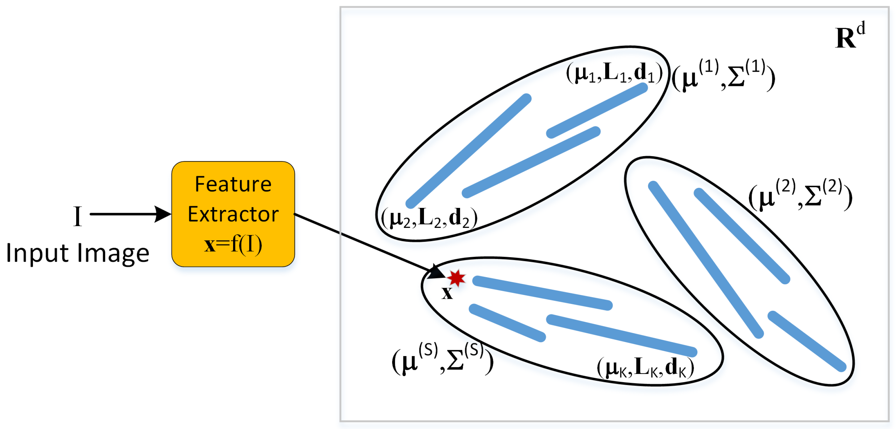
Inspired by our understanding of the human hierarchical representation of objects, this work proposes a hierarchical classification framework called Hierarchical PPCA that exploits the semantic information of image classes. Figure 1 illustrates the hierarchical classification process, where an observation $\mathbf{x}=\mathbf{f}\left(\mathbf{I}\right)$ is first classified and assigned to a super-class $({\mathsf{\mu }}^{\left(s\right)},{\mathsf{\Sigma }}^{\left(s\right)})$ and then classified and assigned to an image class from the image classes belonging to that super-class.

4.1. Hierarchical Classifier

In [26], it was stated that the human cognitive architecture is built up of a hierarchy of multiple system levels. Humans, even babies, use the hierarchical cognition system to conduct categorization without training with huge numbers of images. Inspired by this finding about human hierarchical cognition, the classifier is modeled as a two-level taxonomy. It aims to organize the information with two levels of abstraction.

In the Hierarchical PPCA model, each image class is conceptualized as a Gaussian distribution by Probabilistic Principal Component Analysis (PPCA) [25], as described in Section 3.2.

The first level of the classifier consists of PPCA neurons representing super-classes. The second level of the classifier consists of PPCA neurons encoding information about image classes. The essential assumption is that image classes with similar semantic information cluster together. A cluster is characterized by its centroid, a PPCA Gaussian that we call a super-class. A super-class maintains the least distance to the image classes belonging to the same cluster. If there are K image classes to be classified (e.g., $K=1000$ for ImageNet), they are clustered into S disjoint sets $K_1,\dots ,K_S$ such that:

$${\cup }_{s=1}^S{K}_s=\{1,\dots ,K\}$$

In the framework of Hierarchical PPCA, the first level models (the super-classes) are represented as $({\mathsf{\mu }}^{\left(k\right)},{\mathsf{\Sigma }}^{\left(k\right)})$, with $k\in \{1,\dots ,S\}$, where S is the number of super-classes. For a super-class $s\in \{1,\dots ,S\}$, the corresponding image classes are represented as $({\mathsf{\mu }}_k,{\mathsf{\Sigma }}_k)$ with $k\in K_s$.

4.2. Hierarchical Classification

Given an observation $\mathbf{x}\in {\mathbb{R}}^d$ (obtained from an image $\mathbf{I}\in \mathsf{\Omega }$ using the feature extractor as $\mathbf{x}=\mathbf{f}\left(\mathbf{I}\right)$), the first level classifier aims to find the most likely super-class s for the observation, a process called super-classification. After the sample $\mathbf{x}$ is assigned to a super-class s, the second level of the classifier will find the most likely image class among image classes $k\in K_s$ associated with super-class s. This process is called image classification. Since both level models are Gaussians, we will use the Mahalanobis distance,

$$r(\mathbf{x};\mathsf{\mu },\mathsf{\Sigma })={(\mathbf{x}-\mathsf{\mu })}^T{\mathsf{\Sigma }}^{-1}(\mathbf{x}-\mathsf{\mu })\ge 0,$$

(9)

to measure how well an observation $\mathbf{x}\in {\mathbb{R}}^d$ fits the Gaussian model $(\mathsf{\mu },\mathsf{\Sigma })$, where a smaller score is better. In practice, for classification involving high-dimensional features and PPCA models, we use Equation (7) from Theorem 1 as a computation efficient score computation method.

However, any super-classification failure would result in the failure of the whole classifier. To minimize the impact of such failures, instead of considering a single most likely super-class, the hierarchical classifier will consider a number T of the most likely super-classes, as described in Algorithm 1. In experiments, T was taken in the range of $T\in \{1,2,3,4,5\}$.

Algorithm 1 Hierarchical classification

Input: Observation $\mathbf{x}\in {\mathbb{R}}^d$, super-class models $({\mathsf{\mu }}^{\left(s\right)},{\mathbf{L}}^{\left(s\right)},{\mathbf{d}}^{\left(s\right)}),s\in \{1,\dots ,S\}$, image class models $({\mathsf{\mu }}_k,{\mathbf{L}}_k,{\mathbf{d}}_k),k\in \{1,\dots ,K\}$, clusters $K_s$ such that ${\cup }_{s=1}^S{K}_s=\{1,\dots ,K\}$

Output: Predicted class label $\widehat{k}\in \{1,\dots ,K\}.$

1: Compute the super-class scores $v_s=r(\mathbf{x};{\mathsf{\mu }}^{\left(s\right)},{\mathbf{L}}^{\left(s\right)},{\mathbf{d}}^{\left(s\right)}),s\in \{1,\dots ,S\}$ 2: Find the indices $J\subset \{1,\dots ,S\},\left|J\right|=T$ of the T lowest scores $v_j,j\in J$ 3: Compute the index set $U={\cup }_{j\in J}{K}_j$ 4: Obtain the predicted class label $$\widehat{k}=\underset{k\in U}{\mathrm{argmin}}r(\mathbf{x};{\mathsf{\mu }}_k,{\mathbf{L}}_k,{\mathbf{d}}_k)$$ (10)

4.3. Computation Complexity

The computation demand of a model can be measured by the average number of neurons used in the classification. For an incoming sample feature, a flat classifier requires the computation of the scores for all K image classes to generate the classification output. In contrast, Hierarchical PPCA requires the score computation for all S super-classes and the score computation of the image classes corresponding to the top T super-classes. Let A denote the average number of image classes associated with one super-class. The computation cost for one classification in Hierarchical PPCA is therefore $S+TA$ neurons (score computations).

We use two measures to evaluate the computational cost of Hierarchical PPCA compared with flat classification. The density is defined as

$$\mathrm{density}=\frac{S+TA}{K}.$$

(11)

The inverse of the density measures the increase in speed of Hierarchical PPCA compared to flat classification:

$$\mathrm{speed-up}=K/(S+TA).$$

(12)

Assuming the K image classes are uniformly distributed for the S clusters, then $A\sim K/S$ and the density is

$$\mathrm{density}\sim \frac{S+KT/S}{K}=\frac{S}{K}+\frac{T}{S}.$$

(13)

From an efficiency perspective, the density reaches a minimum when $S=\sqrt{KT}$, where the increase in speed reaches a maximum of $O\left(\sqrt{K/T}\right)$. The experimental results in Section 5.6 match our theoretical derivation.

4.4. Training the Hierarchical Classifier

One important assumption is that image classes with similar semantic information form clusters in the feature space. With this assumption, we adopt a variant of the k-means algorithm to explore the semantic structure of image classes and train the hierarchical classifier. The difference to the standard k-means is that instead of clustering observations, the proposed algorithm clusters image classes encoded as Gaussian distributions. The advantage of this approach is that it only needs to cluster a small number of elements (e.g., 1000 Gaussian distributions for ImageNet) instead of millions of observations. Moreover, this kind of clustering is robust to data imbalances in the classes. The training algorithm is summarized in Algorithm 2.

Algorithm 2 Hierarchical PPCA training

Input: Training observations $({\mathbf{x}}_i,y_i)\in {\mathbb{R}}^d\times \mathbb{Z}$, number S of super-classes, number q of PCs for the image class models, number r of PCs for the super-class models.

Output: Super-class models $({\mathsf{\mu }}^{\left(s\right)},{\mathbf{L}}^{\left(s\right)},{\mathbf{d}}^{\left(s\right)}),s\in \{1,\dots ,S\}$, image class models $({\mathsf{\mu }}_k,{\mathbf{L}}_k,{\mathbf{d}}_k),k\in \{1,\dots ,K\}$.

1: Train the image class Gaussian models $({\mathsf{\mu }}_k,{\mathsf{\Sigma }}_k)$ using Equations (3) and (4). 2: Initialize S super-class models using k- means++ (Section 4.4.1). 3: while not converged do 4:    Assign the image classes $({\mathsf{\mu }}_k,{\mathsf{\Sigma }}_k),k\in \{1,\dots ,K\}$ to the super-classes using Equation (15) 5:    Update the super-class models $({\mathsf{\mu }}^{\left(s\right)},{\mathsf{\Sigma }}^{\left(s\right)}),s\in \{1,\dots ,S\}$ based on the image classes in the same clusters (Section 4.4.3). 6: end while 7: Train the image class PPCA models $({\mathsf{\mu }}_k,{\mathbf{L}}_k,{\mathbf{d}}_k),k\in \{1,\dots ,K\}$ (Section 3.3). 8: Update the super-class PPCA models $({\mathsf{\mu }}^{\left(s\right)},{\mathbf{L}}^{\left(s\right)},{\mathbf{d}}^{\left(s\right)}),s\in \{1,\dots ,S\}$

The training procedure is a generalization of k-means clustering. The clustering subjects are image classes encoded as Gaussian distributions $({\mathsf{\mu }}_k,{\mathsf{\Sigma }}_k)$ instead of vectors. The covariance matrices used for clustering the image classes are the full image covariances ${\mathsf{\Sigma }}_k={\mathbf{C}}_k$ from Equation (4) instead of the PPCA covariances (6).

We innovate with the following modification for the new clustering subjects:

• The distance measure between the image classes, which is used for the k-means++ initialization [27], is replaced by the Bhattacharyya distance (instead of the Mahalanobis distance) between Gaussians (Section 4.4.1).
• The distance measure between an image class and a Gaussian super-class model is the KL divergence, described in Section 4.4.2.
• The Gaussian super-class models are parameterized to minimize the sum of the KL-divergences of the image class models, as described in Section 4.4.3.

These steps will be presented in the following sections.

The second level of the Hierarchical PPCA model contains PPCA models representing information for the image classes. The PPCA neurons are trained by SVD decomposition separately for each class, as described in Section 3.3. The same approach is used to obtain super-class PPCA models from the super-class covariance matrices.

4.4.1. Initialization by k-Means++

The performance of k-means relies significantly on its initialization. In [28], it was shown that the case with the worst running time of the k-means algorithm is super-polynomial in the input size. We adopt the k-means++ [27] initialization method to accelerate the convergence speed and improve clustering performance. The process of k-means++ is detailed in Algorithm 3.

The elements that are clustered are the image classes represented by Gaussian distributions. We adopt the Bhattacharyya distance to measure the pairwise distance between two distributions. For Gaussian distributions $({\mathsf{\mu }}_i,{\mathsf{\Sigma }}_i)$ and $({\mathsf{\mu }}_j,{\mathsf{\Sigma }}_j)$, the Bhattacharyya distance is

$$D_{ij}=\frac{1}{8}{({\mathsf{\mu }}_i-{\mathsf{\mu }}_j)}^T{\mathsf{\Sigma }}^{-1}({\mathsf{\mu }}_i-{\mathsf{\mu }}_j)+\frac{1}{2}ln\frac{\left|\mathsf{\Sigma }\right|}{\sqrt{|{\mathsf{\Sigma }}_i\left|\right|{\mathsf{\Sigma }}_j|}},$$

(14)

where $\mathsf{\Sigma }=\frac{{\mathsf{\Sigma }}_i+{\mathsf{\Sigma }}_j}{2}$.

Algorithm 3 k-means++ centroid initialization

Input: Image classes represented as $({\mathsf{\mu }}_k,{\mathsf{\Sigma }}_k)$$k\in \{1,\dots ,K\}$, number S of clusters

Output. Initial super-class models (centroids) $C_s=({\mathsf{\mu }}^{\left(s\right)},{\mathsf{\Sigma }}^{\left(s\right)})$, $s\in \{1,\dots ,S\}$

1: Randomly pick the first centroid $C_1$ 2: for $i=2$ to S do 3:    Compute the distance between all image classes and the newly selected centroid $C_{i-1}$ using Equation (14) 4:    Generate the discrete distribution on image classes proportional to the distance from each image class to its closest centroid from $\{C_1,\dots ,C_{i-1}\}$ 5:    Sample the image class $({\mathsf{\mu }}_j,{\mathsf{\Sigma }}_j)$ from the discrete distribution generated 6:    Obtain initial centroid $C_i=({\mathsf{\mu }}_j,{\mathsf{\Sigma }}_j)$ 7: end for

4.4.2. Assignment of Image Classes to Clusters

In the training process, the image classes are assigned to the nearest cluster. A distance measure is needed to measure the distance from image classes to the clusters, both of which are characterized by Gaussian distributions. We adopt the Kullback–Leibler (KL) divergence [29], denoted by $D_{KL}(P\Vert Q)$, to measure the distance between image classes and super-classes.

Since all classes are encoded as Gaussian distributions, the KL divergence between a super-class $Q=(\mathsf{\mu },\mathsf{\Sigma })$ and an image class $P=({\mathsf{\mu }}_i,{\mathsf{\Sigma }}_i)$ is [30]

$$\begin{array}{c}\hfill D_{KL}(P\Vert Q)=\frac{1}{2}\{\log \frac{\left|\mathsf{\Sigma }\right|}{|{\mathsf{\Sigma }}_i|}-d+\mathrm{Tr}\left[{\mathsf{\Sigma }}^{-1}{\mathsf{\Sigma }}_i\right]\}+{({\mathsf{\mu }}_i-\mathsf{\mu })}^T{\mathsf{\Sigma }}^{-1}({\mathsf{\mu }}_i-\mathsf{\mu })/2\end{array}$$

(15)

4.4.3. Super-Class Model Update

By our assumption of image classes, the super-class model is the centroid of the corresponding cluster, i.e., the Gaussian distribution that has the smallest sum of the distances to the image classes within the same cluster.

The image classes within a cluster C are normal distributions $\mathcal{N}({\mathsf{\mu }}_i,{\mathsf{\Sigma }}_i),i\in C$. The corresponding super-class model is a normal distribution $\mathcal{N}(\mathsf{\mu },\mathsf{\Sigma })$ so that the sum of the distances from the image classes to the super-class

$$D(\mathsf{\mu },\mathsf{\Sigma })=\sum _{i\in C}{D}_{KL}(\mathcal{N}({\mathsf{\mu }}_i,{\mathsf{\Sigma }}_i)\Vert \mathcal{N}(\mathsf{\mu },\mathsf{\Sigma }))$$

(16)

is minimized, where $D_{KL}(P\Vert Q)$ is defined in Equation (15).

The following theorem gives a closed-form solution of the minimization.

Theorem 2.

The Gaussian distribution $\mathcal{N}(\mathsf{\mu },\mathsf{\Sigma })$ that minimizes $D(\mathsf{\mu },\mathsf{\Sigma })$ from Equation (16) has mean

$$\mathsf{\mu }=\frac{1}{\left|C\right|}\sum _{i\in C}{\mathsf{\mu }}_i,$$

(17)

and covariance

$$\mathsf{\Sigma }=\frac{1}{\left|C\right|}\sum _{i\in C}[({\mathsf{\mu }}_i-\mathsf{\mu }){({\mathsf{\mu }}_i-\mathsf{\mu })}^T+{\mathsf{\Sigma }}_i].$$

(18)

Proof. 

From [30], the KL divergence between normal distributions $P=\mathcal{N}({\mathsf{\mu }}_i,{\mathsf{\Sigma }}_i)$ and $Q=\mathcal{N}(\mathsf{\mu },\mathsf{\Sigma })$ is

$$D_{KL}\left(P\right|\left|Q\right)=\frac{1}{2}[\log \frac{\left|\mathsf{\Sigma }\right|}{|{\mathsf{\Sigma }}_i|}-d+{({\mathsf{\mu }}_i-\mathsf{\mu })}^T{\mathsf{\Sigma }}^{-1}({\mathsf{\mu }}_i-\mathsf{\mu })+Tr\left\{{\mathsf{\Sigma }}^{-1}{\mathsf{\Sigma }}_i\right\}],$$

(19)

so the sum is

$$D(\mathsf{\mu },\mathsf{\Sigma })=\frac{1}{2}\sum _{i\in C}\{\log \frac{\left|\mathsf{\Sigma }\right|}{|{\mathsf{\Sigma }}_i|}-d+{({\mathsf{\mu }}_i-\mathsf{\mu })}^T{\mathsf{\Sigma }}^{-1}({\mathsf{\mu }}_i-\mathsf{\mu })+Tr\left({\mathsf{\Sigma }}^{-1}{\mathsf{\Sigma }}_i\right)\}.$$

(20)

Setting the partial derivative of $D(\mathsf{\mu },\mathsf{\Sigma })$ with respect to $\mathsf{\mu }$,

$$\frac{\partial }{\partial \mathsf{\mu }}D(\mathsf{\mu },\mathsf{\Sigma })=\sum _{i\in C}{\mathsf{\Sigma }}^{-1}({\mathsf{\mu }}_i-\mathsf{\mu }),$$

(21)

to zero, we obtain $\mathsf{\mu }=\frac{1}{\left|C\right|}{\sum }_{i\in C}{\mathsf{\mu }}_i$.

${(\mathbf{x}-\mathsf{\mu })}^T{\mathsf{\Sigma }}^{-1}(\mathbf{x}-\mathsf{\mu })$ can be written as $Tr\left[{(\mathbf{x}-\mathsf{\mu })}^T{\mathsf{\Sigma }}^{-1}(\mathbf{x}-\mathsf{\mu })\right]$; thus, the third term of Equation (20) can be written as

$$\sum _{i\in C}Tr\left[{({\mathsf{\mu }}_i-\mathsf{\mu })}^T{\mathsf{\Sigma }}^{-1}({\mathsf{\mu }}_i-\mathsf{\mu })\right]=\sum _{i\in C}Tr\left[({\mathsf{\mu }}_i-\mathsf{\mu }){({\mathsf{\mu }}_i-\mathsf{\mu })}^T{\mathsf{\Sigma }}^{-1}\right]$$

(22)

Thus, the distance (20) can be written as

$$\begin{array}{cc}\hfill D(\mathsf{\mu },\mathsf{\Sigma })& =\frac{1}{2}\sum _{i\in C}\left(\log \frac{\left|\mathsf{\Sigma }\right|}{|{\mathsf{\Sigma }}_i|}+Tr\left[({\mathsf{\mu }}_i-\mathsf{\mu }){({\mathsf{\mu }}_i-\mathsf{\mu })}^T{\mathsf{\Sigma }}^{-1}\right]+Tr\left\{{\mathsf{\Sigma }}^{-1}{\mathsf{\Sigma }}_i\right\}\right)\hfill \\ \hfill & =\frac{1}{2}\sum _{i\in C}\log \frac{\left|\mathsf{\Sigma }\right|}{|{\mathsf{\Sigma }}_i|}+\frac{1}{2}Tr\left\{\sum _{i\in C}[({\mathsf{\mu }}_i-\mathsf{\mu }){({\mathsf{\mu }}_i-\mathsf{\mu })}^T+{\mathsf{\Sigma }}_i]{\mathsf{\Sigma }}^{-1}\right\}\hfill \end{array}$$

(23)

Therefore, the partial derivative of $D(\mathsf{\mu },\mathsf{\Sigma })$ with respect to $\mathsf{\Sigma }$ is

$$2\frac{\partial }{\partial \mathsf{\Sigma }}D(\mathsf{\mu },\mathsf{\Sigma })=\left|C\right|{\mathsf{\Sigma }}^{-1}-{\mathsf{\Sigma }}^{-1}\sum _{i\in C}[({\mathsf{\mu }}_i-\mathsf{\mu }){({\mathsf{\mu }}_i-\mathsf{\mu })}^T+{\mathsf{\Sigma }}_i]{\mathsf{\Sigma }}^{-1}$$

(24)

Setting $\frac{\partial }{\partial \mathsf{\Sigma }}D(\mathsf{\mu },\mathsf{\Sigma })=0$ and multiplying the left and the right by $\mathsf{\Sigma }$, we obtain

$$\mathsf{\Sigma }=\frac{1}{\left|C\right|}\sum _{i\in C}[({\mathsf{\mu }}_i-\mathsf{\mu }){({\mathsf{\mu }}_i-\mathsf{\mu })}^T+{\mathsf{\Sigma }}_i].$$

(25)

□

The super-class PPCA models $({\mathsf{\mu }}^{\left(s\right)},{\mathbf{L}}^{\left(s\right)},{\mathbf{d}}^{\left(s\right)})$ can be computed by writing $\mathbf{V}\mathbf{S}{\mathbf{V}}^T={\mathsf{\Sigma }}^{\left(s\right)}$ by SVD, and obtaining ${\mathbf{L}}^{\left(s\right)}$ as the first q columns of $\mathbf{V}$ and ${\mathbf{d}}^{\left(s\right)}$ as the first q diagonal elements of $\mathbf{S}$.

5. Experiments

Experiments were conducted to compare the accuracy and computation efficiency of Hierarchical PPCA with the flat PPCA classifier, i.e., the one-level classifier containing the same PPCA image models but where the classification $y={\mathrm{argmin}}_{k}r(\mathbf{x};{\mathsf{\mu }}_k,{\mathbf{L}}_k,{\mathbf{d}}_k)$ finds the minimum score for an observation $\mathbf{x}=\mathbf{f}\left(\mathbf{I}\right),\mathbf{I}\in \mathsf{\Omega }$ among all classes $k\in \{1,...,K\}$. The experiments were designed to explore how some of the main parameters such as the number S of super-classes, the number of principal components, and the parameter T from Algorithm 1 influence accuracy and computation efficiency.

5.1. Datasets

Experiments were conducted on three standard datasets: ImageNet-100, ImageNet-1k (ILSVRC 2016) [31], and ImageNet-10k. ImageNet-100 is a subset of ImageNet-1k with only 100 classes, randomly sampled from the original 1000 classes. ImageNet-10k is the subset of the whole ImageNet [31] that contains all 10,450 classes with at least 450 training observations. They are standard image datasets that are adopted to prove the robustness and facilitate comparisons. All results are reported as averages of five independent runs for better reproducibility. Each of these datasets has a separate test set with 50 observations per class; thus, the ImageNet-1k has 50,000 test observations, and so on.

5.2. Feature Extractor

The feature extractor $\mathbf{f}:\mathsf{\Omega }\to {\mathbb{R}}^d$ used in this work is the ResNet50x4 from CLIP (Contrastive Language-Image Pre-Training) [32]. CLIP models are pairs of image embedding and language embedding models, trained on 400 million pairs of images and their corresponding captions. They are trained on a wide variety of images with a wide variety of natural language supervision that is abundantly available on the internet. By design, the network can be instructed in natural language to perform a great variety of classification benchmarks, without directly optimizing for the benchmark’s performance. As such, it was not trained or fine-tuned on the three evaluation datasets. CLIP models with different numbers of parameters were also used in [23] for classification using a simple k-nearest neighbor classifier.

The choice of the feature extractor is important for the validity of the assumption made for Hierarchical PPCA, which is that semantically similar classes cluster together.

5.3. Evaluation Measures

• Efficiency Measure. There are two efficiency measures: density and speed increase. The density evaluates how much less computation is required for classification using Hierarchical PPCA compared to flat classification. The theoretical definition and analysis were presented in Section 4.3. In practice, density is defined as

  $$\mathrm{density}=\frac{S+A}{K}$$

  (26)

  where A is the average number of image classes used, S is the number of super-classes, and K is the total number of classes. The speed increase is the inverse of density and measures the computational efficiency of Hierarchical PPCA. The theoretical analysis from Section 4.3 indicates that the density reaches a minimum and the speed increase is at a maximum when $S=\sqrt{KT}$.
• Super-class accuracy. The super-classes are constructed without human annotation, using k-means clustering, by exploring the semantic relations between the image classes. Classifying an observation to the wrong super-class would result in a failure in the overall classification of this observation. The super-class accuracy measures the top-T classification accuracy of the level 1 (super-class) classifier.

5.4. Raw Data Clustering

In Hierarchical PPCA, the super-classes are learned by clustering the image classes, which are parameterized as Gaussian distributions. Another hierarchical method that will be evaluated is raw data clustering, which is similar to Hierarchical PPCA, but the super-class models are obtained from clustering a subsample of observations from the image classes instead of clustering the Gaussian models of image classes.

In this experiment, 20 images are randomly sampled from each image class, obtaining a sample of $20K$ images, where K is the number of image classes. The images are clustered in S clusters using the standard k-means clustering algorithm. Then, each image class is assigned to the cluster containing the maximum number of its images. The super-class models are updated for each cluster as described in Section 4.4.3.

5.5. Main Results

For completeness, we will also evaluate a standard linear projection head, which is a fully connected layer trained to predict the class label from the same feature vector $\mathbf{x}=\mathbf{f}\left(\mathbf{i}\right)\in {\mathbb{R}}^d$ as the Hierarchical PPCA classifiers for an image $\mathbf{I}$. These linear projection classifiers were trained using the Adam optimizer [33] and the cross-entropy loss, starting with a learning rate of 0.03. The models on ImageNet-100 and ImageNet-1k were trained for 300 epochs and the learning rate was reduced by 5 every 50 epochs, while the model on ImageNet-10k was trained for 100 epochs and the learning rate was reduced by 5 every 15 epochs.

The main comparison of the Hierarchical PPCA, Hierarchical PPCA with raw data clustering, flat PPCA and the linear projection head in terms of test accuracy and computational efficiency is shown in

Table 1. Evaluation in terms of test accuracy and speed increase vs. flat classification and linear projection head of the proposed Hierarchical PPCA Algorithm 1 with $T=1$ and $T=5$ and $q=r=50$. Shown also are the raw data clustering test accuracy and speed increase results. Results are averages over five independent runs and the standard deviations are shown in parentheses.

	ImageNet-100		ImageNet-1k		ImageNet-10k
	Accuracy	Speed Increase	Accuracy	Speed Increase	Accuracy	Speed Increase
Linear Proj. Head	0.923 (0.009)	1.0	0.720 (0.000)	1.0	0.370 (0.000)	1.0
Flat PPCA Clf.	0.920 (0.013)	1.0	0.736	1.0	0.384	1.0
HPPCA $T=1$	0.902 (0.019)	3.9 (0.4)	0.672 (0.005)	13.8 (0.3)	0.319 (0.003)	41.6 (3.8)
HPPCA $T=5$	0.920 (0.013)	1.4 (0.1)	0.734 (0.000)	4.7 (0.2)	0.376 (0.000)	14.1 (0.9)
Raw data clust. $T=1$	0.902 (0.017)	4.5 (0.4)	0.664 (0.005)	14.7 (0.2)	0.308 (0.001)	47.6 (0.4)
Raw data clust. $T=5$	0.920 (0.013)	1.5 (0.1)	0.734 (0.000)	5.1 (0.1)	0.372 (0.000)	16.1 (0.2)

. The results are averages of five independent runs with the standard deviation shown in parentheses. The flat PPCA classifier is deterministic (being obtained by SVD from the observations of each class independently), so only the ImageNet-100 accuracy has non-zero variance, due to the random subsampling of the 100 classes out of 1000.

From Table 1, we see that for ImageNet-1k and ImageNet-10k datasets, when $T=5$, the Hierarchical PPCA surpasses the linear projection classifier both in terms of accuracy and computational efficiency. Compared to flat PPCA, the Hierarchical PPCA results are slightly inferior.

Table 2. Comparison between the accuracy of Hierarchical PPCA when clustering Gaussians vs. clustering raw data.

	ImageNet-100			ImageNet-1k			ImageNet-10k
$\mathit{T}$	Flat	Raw Data	Gaussians	Flat	Raw Data	Gaussians	Flat	Raw Data	Gaussians
1	0.920 (0.013)	0.902 (0.017)	0.902 (0.019)	0.736	0.664 (0.005)	0.672 (0.005)	0.384	0.308 (0.001)	0.319 (0.003)
2	-	0.918 (0.013)	0.918 (0.013)	-	0.715 (0.003)	0.718 (0.003)	-	0.348 (0.001)	0.356 (0.001)
3	-	0.920 (0.013)	0.919 (0.013)	-	0.727 (0.001)	0.728 (0.001)	-	0.361 (0.001)	0.368 (0.001)
4	-	0.920 (0.013)	0.920 (0.013)	-	0.732 (0.000)	0.732 (0.000)	-	0.368 (0.000)	0.373 (0.000)
5	-	0.920 (0.013)	0.920 (0.013)	-	0.734 (0.000)	0.734 (0.000)	-	0.372 (0.000)	0.376 (0.000)

shows detailed results on Hierarchical PPCA with raw data and with Gaussians with $T\in \{1,2,3,4,5\}$. It indicates that clustering Gaussians is usually better than clustering raw data. On ImageNet-1k, the performance of clustering from raw data is slightly inferior to Hierarchical PPCA for $T\in \{1,2,3\}$. On ImageNet-10k, clustering raw data is consistently inferior to clustering Gaussians.

5.6. Hyperparameter Analysis

A hyperparameter analysis investigates the importance of the number S of super-classes, the parameter T of Algorithm 1, and the number of PCA directions of the PPCA models in the speed and accuracy of the Hierarchical PPCA method.

5.6.1. Number S of Super-Classes

The super-classes represent the general concepts in the Hierarchical PPCA approach, which are used to speed up classification. The number of super-classes S is an important factor for computation efficiency and overall accuracy.

Table 3. Evaluation of speed increases and accuracy for different numbers S of super-classes, when the number of PCA components is $q=r=50$.

S	Density	Speed Increase	Accuracy	Super Accuracy
ImageNet-100, $T=4$
Flat	1.0	1.0	0.920 (0.013)	-
5	0.905 (0.039)	1.1 (0.0)	0.920 (0.013)	1.000 (0.000)
10	0.607 (0.070)	1.7 (0.2)	0.920 (0.013)	0.999 (0.000)
20	0.492 (0.025)	2.0 (0.1)	0.920 (0.013)	0.996 (0.002)
ImageNet-1k, $T=5$
Flat	1.0	1.0	0.736	-
10	0.567 (0.019)	1.8 (0.1)	0.736 (0.000)	0.998 (0.000)
20	0.313 (0.019)	3.2 (0.2)	0.735 (0.000)	0.989 (0.002)
33	0.212 (0.007)	4.7 (0.2)	0.734 (0.000)	0.979 (0.003)
40	0.192 (0.010)	5.2 (0.3)	0.734 (0.000)	0.976 (0.002)
50	0.178 (0.007)	5.6 (0.2)	0.733 (0.000)	0.973 (0.002)
66	0.166 (0.003)	6.0 (0.1)	0.733 (0.001)	0.968 (0.002)
100	0.165 (0.003)	6.1 (0.1)	0.734 (0.000)	0.963 (0.001)
ImageNet-10k, $T=5$
Flat	1	1	0.384	-
50	0.117 (0.003)	8.6 (0.2)	0.379 (0.000)	0.952 (0.002)
100	0.071 (0.005)	14.1 (0.9)	0.376 (0.000)	0.927 (0.003)
200	0.050 (0.001)	20.0 (0.3)	0.375 (0.000)	0.898 (0.002)
300	0.050 (0.000)	19.9 (0.1)	0.375 (0.000)	0.883 (0.001)

shows an evaluation of the test accuracy and speed increases for different numbers of super-classes for the three datasets.

ImageNet-100 contains 100 image classes. The experiment adopts three values for S, namely, $S\in \{5,10,20\}$. The density does not decrease monotonically with increasing S. The speed increase reaches a maximum of 2.0 when $S=20$. The super-class test accuracy for the three values of S is larger than the flat accuracy, indicating unsupervised generated super-classes are interpretable for classification. The super accuracy decreases monotonically with an increase in S. The result indicates that the overall accuracy has a negative correlation with the speed increase coefficient.

For ImageNet-1k, we adopted seven values for S, $S\in \{10,20,33,40,50,66,100\}$, since $K=1000$. From the perspective of efficiency, the speed increase coefficient reaches a maximum when $S=100$, which is higher than $\sqrt{K}$, the theoretical optimum derived in Section 4.3. The efficiency approximately conforms to the theoretical derivation. The accuracy and super accuracy reach their maximum when $S=10$ and are negatively correlated with S. The result follows a similar pattern to the result of ImageNet-100.

For ImageNet-10k, considering that K = 10,450, we consider the following S values: $S\in \{50,100,200,300\}$. From the perspective of efficiency, the speed increase coefficient reaches the optimum of 20 when $S=200$, which is approximately $\sqrt{K}$. The Hierarchical PPCA reaches the best accuracy of 0.379 when $S=50$ with a speed increase of $8.6$.

In summary, the S experiments indicate that the efficiency of the Hierarchical PPCA for $T=5$ reaches an optimum when $S=\sqrt{K}$. Overall, the accuracy and super accuracy have a negative correlation with S. The overall accuracy of Hierarchical PPCA is slightly inferior to flat classification. The super accuracy results indicate that super-classes are interpretable for classification.

5.6.2. Improving the Super Accuracy

Hierarchical PPCA assigns the samples to the T most likely super-classes. Super-classification failure significantly damages the overall classification accuracy. The overall error is composed of errors from image classification and errors from super-class classification. The Hierarchical PPCA can increase its super-class accuracy by considering samples from multiple most likely clusters. Experiments aim to explore whether increasing T benefits the overall accuracy and the impact on the classification speed.

Table 4. Evaluation of speed increases and accuracy for different values of the parameter T from Algorithm 1, when the number of PC components is $q=r=50$.

T	Density	Speed Increase	Accuracy	Super Accuracy
ImageNet-100, $S=10$
Flat	1.0	1.0	0.920 (0.013)	-
1	0.257 (0.029)	3.9 (0.4)	0.902 (0.019)	0.953 (0.011)
2	0.391 (0.057)	2.6 (0.4)	0.918 (0.013)	0.989 (0.002)
3	0.502 (0.062)	2.0 (0.3)	0.919 (0.013)	0.996 (0.001)
4	0.607 (0.070)	1.7 (0.2)	0.920 (0.013)	0.999 (0.000)
5	0.713 (0.074)	1.4 (0.1)	0.920 (0.013)	0.999 (0.000)
ImageNet-1k, $S=33$
Flat	1.0	1.0	0.736	-
1	0.073 (0.002)	13.8 (0.3)	0.672 (0.005)	0.822 (0.008)
2	0.108 (0.004)	9.2 (0.3)	0.718 (0.003)	0.922 (0.004)
3	0.144 (0.006)	7.0 (0.3)	0.728 (0.001)	0.954 (0.003)
4	0.178 (0.006)	5.6 (0.2)	0.732 (0.000)	0.970 (0.002)
5	0.212 (0.007)	4.7 (0.2)	0.734 (0.000)	0.979 (0.003)
ImageNet-10k, $S=100$
Flat	1.0	1.0	0.384	-
1	0.024 (0.002)	41.6 (3.8)	0.319 (0.003)	0.694 (0.010)
2	0.037 (0.003)	27.5 (2.0)	0.356 (0.001)	0.827 (0.007)
3	0.048 (0.003)	20.8 (1.4)	0.368 (0.001)	0.880 (0.005)
4	0.060 (0.004)	16.8 (1.1)	0.373 (0.000)	0.909 (0.004)
5	0.071 (0.005)	14.1 (0.9)	0.376 (0.000)	0.927 (0.003)

shows the effectiveness of this strategy. The overall accuracy increases monotonically with T. For ImageNet-100, Hierarchical PPCA reaches the flat classification accuracy when $T=4$. Meanwhile, the super-class accuracy increases significantly, from 0.95 to 0.999. Compared to flat classification, Hierarchical PPCA can reach a similar accuracy while only using $61\%$ of the PPCA neurons. Table 4 also indicates that the density increases linearly with T.

The results on ImageNet-1k with $S=33$ follow a similar pattern. The accuracy and super accuracy follow a positive correlation with T. The overall accuracy increased from 0.672 to 0.718 as T increased to 2. The Hierarchical PPCA achieves a performance close to that of flat classification when T reaches 5 while the density is 0.212. Hierarchical PPCA can achieve a similar performance with less than $25\%$ of neurons.

The experiment on ImageNet-10k was conducted with $S=100$. The overall accuracy increased from 0.319 to 0.376 as T increased to 5. The density increases linearly with T.

In summary, the strategy of increasing T elevates the super-class accuracy and overall accuracy by sacrificing some computational efficiency. The experimental results indicate that for medium datasets like ImageNet-100 and ImageNet-1k, Hierarchical PPCA can achieve equivalent results with no more than $20\%$ of the neurons used. The computational cost increases approximately linearly with increasing T.

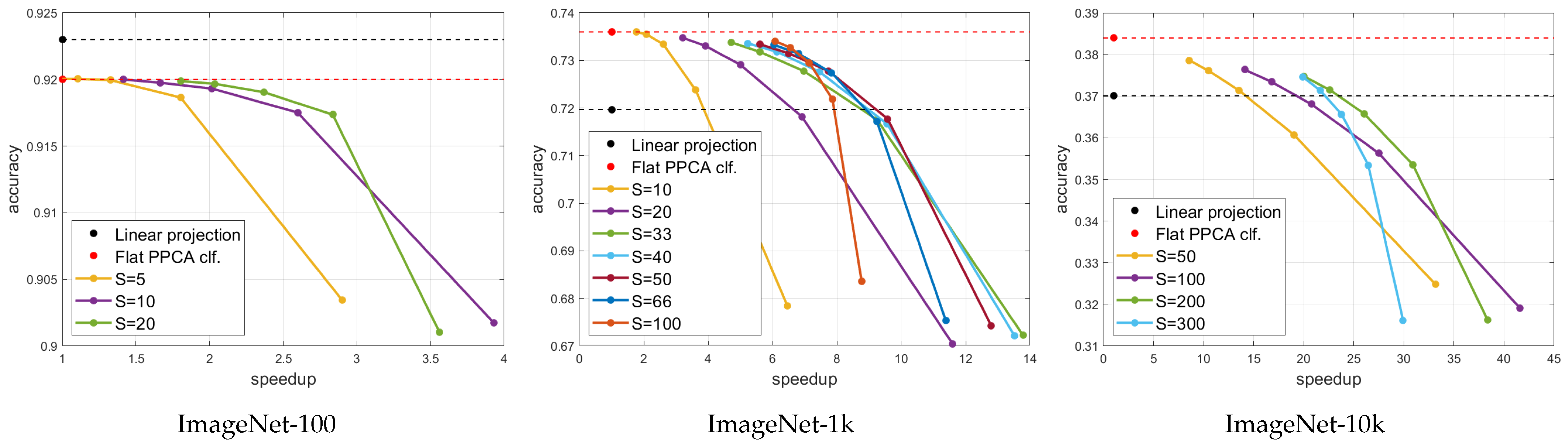
Figure 2 reveals the relationship between the accuracy and speed increase for different numbers S of super-classes, where each curve represents the accuracy vs. speedup for one value of S and for $T\in \{1,2,3,4,5\}$. The relationship between the accuracy and speed increase coefficient follows a negative logarithmic trend. Compared to flat classification, hierarchical classification can obtain a comparable accuracy with between a 2-fold and 20-fold speed increase, depending on the dataset. Compared to the standard linear projection classifier, Hierarchical PPCA has a superior accuracy for large datasets, with an 8–20-fild speed increase.

5.6.3. Number of Principal Components

The number of principal components (PCs) is an essential hyperparameter. Theoretically, q represents the dimension of the (linear) manifold to the observations of each class. Furthermore, the case considered is $q=0$, in which the PPCA neurons will degenerate into radial basis function (RBF) neurons [34]:

$$r(\mathbf{x};{\mathsf{\mu }}_k,{\mathsf{\Sigma }}_k)={\parallel \mathbf{x}-{\mathsf{\mu }}_k\parallel }^2,$$

(27)

where classification is based on the nearest Euclidean distance to the mean ${\mathsf{\mu }}_k$ instead of the Mahalanobis distance (2). The experiment aims to explore how the number of principal components influences accuracy.

Actually, there are two PC parameters: the number q of PCs in the image class PPCA models and the number r of PCs in the super-class PPCA models.

• Experiment 1, r = q. In the first experiment, we set $r=q$ (same number of PCs for classes and super-classes) and varied q.

  Table 5. Accuracy vs. number q of principal components.

  			q
  Method	$\mathit{S}$	$\mathit{T}$	0	10	20	50	100	200
  ImageNet-100
  flat classification	-	-	0.882 (0.018)	0.915 (0.012)	0.920 (0.011)	0.920 (0.013)	0.919 (0.012)	0.918 (0.012)
  HPPCA, $r=q$	10	1	0.780 (0.037)	0.883 (0.023)	0.896 (0.019)	0.902 (0.019)	0.903 (0.016)	0.902 (0.016)
  HPPCA, $r=q$	10	5	0.881 (0.018)	0.915 (0.012)	0.920 (0.011)	0.920 (0.013)	0.919 (0.012)	0.918 (0.012)
  ImageNet-1k
  flat classification	-	-	0.648	0.719	0.732	0.736	0.735	0.735
  HPPCA, $r=q$	33	1	0.492 (0.007)	0.621 (0.005)	0.653 (0.005)	0.672 (0.005)	0.674 (0.004)	0.674 (0.005)
  HPPCA, $r=q$	33	5	0.635 (0.002)	0.713 (0.001)	0.728 (0.000)	0.734 (0.000)	0.734 (0.000)	0.734 (0.000)
  ImageNet-10k
  flat classification	-	-	0.288	0.364	0.378	0.384	0.382	0.380
  HPPCA, $r=q$	100	1	0.207 (0.004)	0.284 (0.003)	0.305 (0.003)	0.319 (0.003)	0.320 (0.002)	0.317 (0.002)
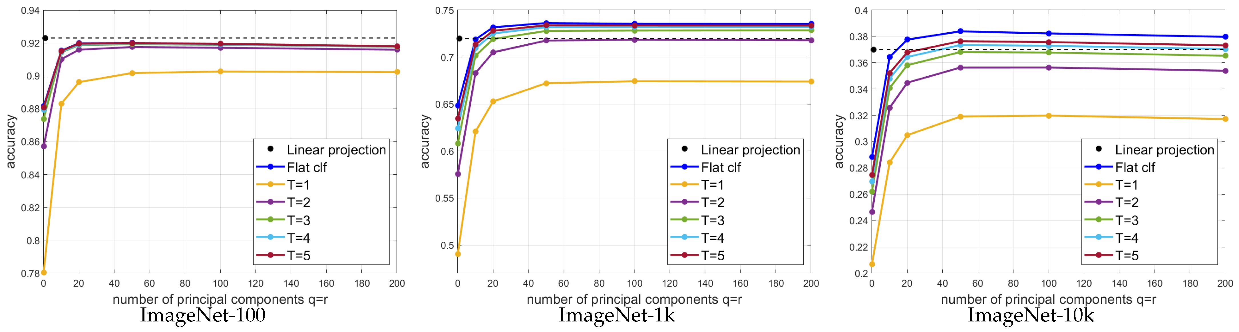
  HPPCA, $q=r$	100	5	0.275 (0.001)	0.352 (0.000)	0.368 (0.000)	0.376 (0.000)	0.376 (0.000)	0.373 (0.000)

  and Figure 3 present the accuracy for different numbers q of PCs used in both the image class and the super-class models ($r=q$). The overall accuracy of Hierarchical PPCA and flat classification does not increase with q monotonically. There is an optimum number of principal components where the overall accuracy reaches a maximum. This optimum point indicates the classifier’s capacity of utilizing variation to improve the classification. The optimum point for flat classification is $q=50$ and for Hierarchical PPCA, the optimum point is $q=r=50$. Figure 3 indicates that Hierarchical PPCA with $T=5$ starts to surpass the linear projection head on accuracy when q reaches 20. With more variation, Hierarchical PPCA performs better than the linear projection head. When $q=0$, the PPCA neurons degrade to RBF neurons. Table 5 shows that PPCA neurons are superior to RBF neurons for both flat and hierarchical classifiers.
• Experiment 2, changing r when q = 50. Super-classes represent more general concepts in Hierarchical PPCA. They are generated by the minimization of the sum of the distance to the image classes. In Experiment 1 above, we explored the relationship between the number of principal components for all PPCA neurons ($q=r$) and the overall accuracy. However, the super-classes may have different semantic properties than image classes. This experiment is designed to explore how the amount of variation encoded for super-classes influences the overall accuracy. We restrict the number of PCs q for the image classes to $q=50$, which is the optimum point for flat classifiers, while changing the number r of PCs for the super-classes.

Table 6. Accuracy vs. number r of principal components for super classification.

			r
Method	$\mathit{S}$	$\mathit{T}$	0	10	20	50	100	200
ImageNet-100
flat clf. $q=r$	-	-	0.882 (0.018)	0.915 (0.012)	0.920 (0.011)	0.920 (0.013)	0.919 (0.012)	0.918 (0.012)
HPPCA, $q=50$	10	5	0.919 (0.013)	0.920 (0.012)	0.920 (0.012)	0.920 (0.013)	0.920 (0.012)	0.920 (0.012)
HPPCA, $q=r$	10	5	0.881 (0.018)	0.915 (0.012)	0.920 (0.011)	0.920 (0.013)	0.919 (0.012)	0.918 (0.012)
ImageNet-1k
flat clf. $q=r$	-	-	0.648	0.719	0.732	0.736	0.735	0.735
HPPCA, $q=50$	33	5	0.715 (0.004)	0.730 (0.001)	0.732 (0.000)	0.734 (0.000)	0.734 (0.000)	0.734 (0.000)
HPPCA, $q=r$	33	5	0.635 (0.002)	0.713 (0.001)	0.728 (0.000)	0.734 (0.000)	0.734 (0.000)	0.734 (0.000)
ImageNet-10k
flat classification	-	-	0.288	0.364	0.378	0.384	0.382	0.380
HPPCA, $q=50$	100	5	0.357 (0.001)	0.370 (0.000)	0.374 (0.000)	0.376 (0.000)	0.377 (0.000)	0.377 (0.000)
HPPCA, $q=r$	100	5	0.275 (0.001)	0.352 (0.000)	0.368 (0.000)	0.376 (0.000)	0.376 (0.000)	0.373 (0.000)

indicates that the overall accuracy does not change significantly with the number r of PCs for the super-classes as long as $r\ge 20$. In comparison with the other experiment and with flat classification, we can conclude that changing the variation encoded for super-classes does not influence the classification much. Super-classes have a different semantic property from image classes and the super classification is not sensitive to changing the number of principal components like image classes.

To reveal the semantic characteristics of PPCA neurons, we explore the overall accuracy when a small amount of variation is encoded for super-classes, i.e., $r\le 3$, keeping $q=50$ and $T=5$.

Table 7. Hierarchical PPCA accuracy vs. number r of principal components for super classification, when $T=5,q=50$.

	r
Dataset	0PC	1PC	2PC	3PC
ImageNet-100 Overall Accuracy	0.919 (0.013)	0.919 (0.013)	0.920 (0.013)	0.920 (0.012)
ImageNet-100 Speed-up	1.4 (0.1)	1.4 (0.1)	1.4 (0.1)	1.4 (0.1)
ImageNet-1k Overall Accuracy	0.715 (0.004)	0.719 (0.003)	0.722 (0.002)	0.724 (0.002)
ImageNet-1k Speed-up	4.6 (0.2)	4.6 (0.2)	4.6 (0.2)	4.6 (0.2)
ImageNet-10k Overall Accuracy	0.357 (0.001)	0.362 (0.001)	0.364 (0.001)	0.365 (0.001)
ImageNet-10k Speed-up	14.2 (1.0)	14.1 (0.9)	14.1 (0.9)	14.2 (0.9)

reveals that the performance of the PPCA neurons is better than RBF neurons for super classification. For all three datasets, but especially large-scale datasets like ImageNet-1k and ImageNet-10k, more encoded information facilitates the super classification, thus improving the overall accuracy.

6. Conclusions and Future Work

This paper introduced a method for fast image classification called Hierarchical PPCA, aimed at classifying data with a large number of classes. The framework adopts probabilistic PCA as a class model for the classifier and clusters the image classes using a modified k-means approach into a small number of super-classes. During classification, the hierarchical model first classifies the data into a small number of super-classes, then only activates the corresponding image class models after super-classification. For large-scale datasets without hierarchical annotation, Hierarchical PPCA can achieve superior accuracy with a fraction of the computational cost. The proposed Hierarchical PPCA therefore gives a positive answer to the research question from Section 1, since the hierarchical organization speeds up classification for K classes from $O\left(K\right)$ to $O\left(\sqrt{K}\right)$, while still outperforming a standard linear projection classifier.

Compared with RBF neurons, the PPCA neurons are capable of modeling the complexity of semantic variation to gain a superior classification accuracy. Hierarchical PPCA has a stronger capacity to utilize variation to aid in classification and computation efficiency. We have noticed that, with fewer training samples, Hierarchical PPCA can achieve a considerable performance for large-scale datasets.

Finally, we want to point out some of the limitations of the proposed Hierarchical PPCA method. First, since it depends on a self-trained feature extractor, it can only be as good as the feature extractor allows. A better feature extractor would allow for obtaining even better classification results. Second, it might fail to separate very similar classes such as “male” vs. “female”, where a special classifier would need to be trained to separate them.

In the future, we plan to further expand the Hierarchical PPCA model to handle more than 100,000 classes with a large range of sizes, from between two and ten observations per class to thousands of observations per class.