

Single-Stage Pose Estimation and Joint Angle Extraction Method for Moving Human Body


Abstract
:1. Introduction
- (1)
- The feature fusion module has been refined using a cutting-edge strategy, bolstering the network’s capability to discern diminutive targets.
- (2)
- We have integrated the mc2f module, which autonomously prioritizes various features based on their relevance.
- (3)
- Leveraging pose estimation, we extract angular data within the motion setting and apply fitting adjustments to further refine feature information accuracy.
2. Related Work
2.1. Human Body Posture Estimation
2.2. Human Pose Loss Function Formulation and Human Pose Estimation Loss
2.3. Human Reconstruction
3. Proposed Method
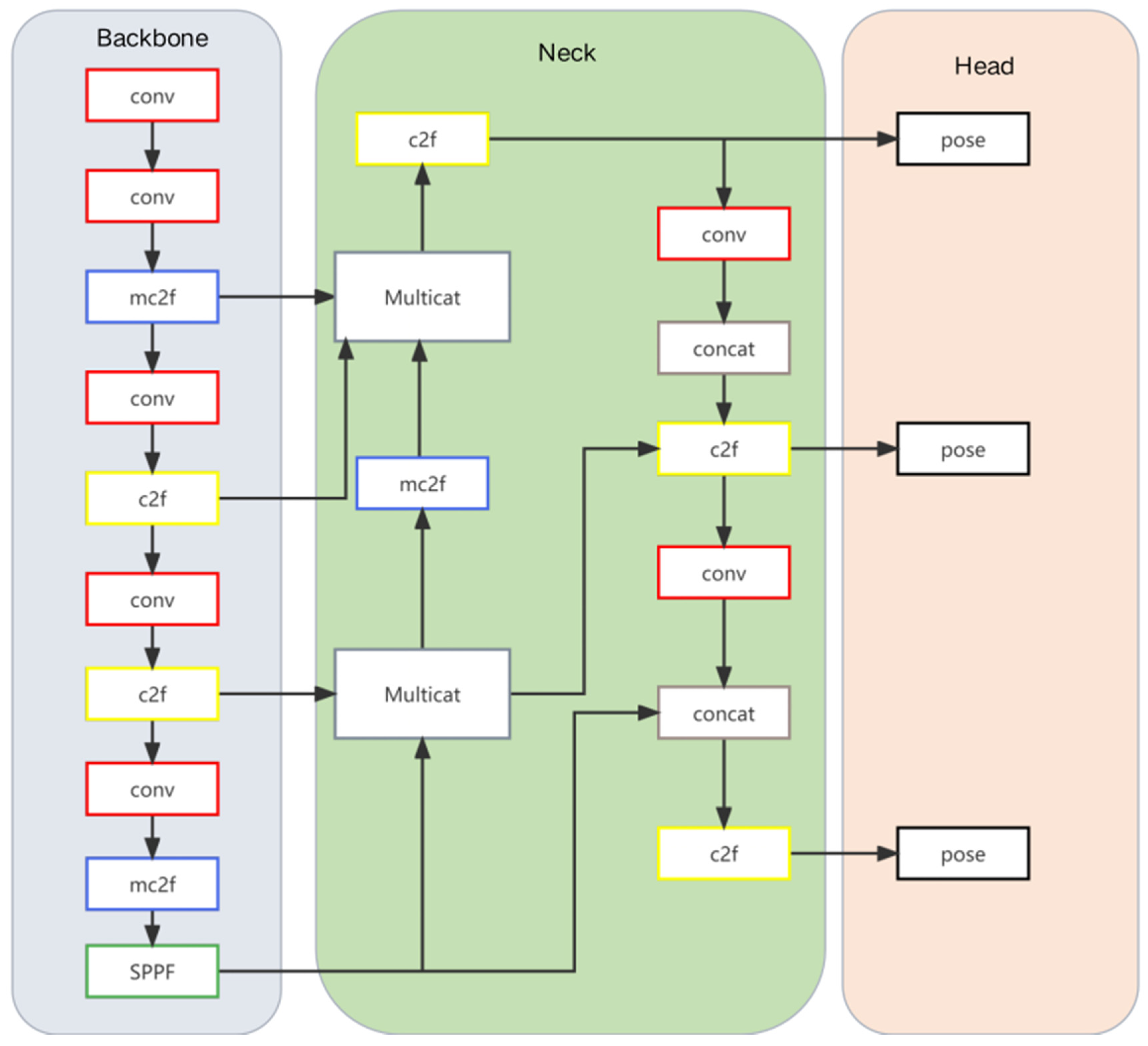
3.1. Yolov8-sp
- (1)
- Incorporation of a three-dimensional cross-scale feature information fusion MultiCat module.
- (2)
- Substitution of the original C2F module with the advanced MC2F within the backbone.
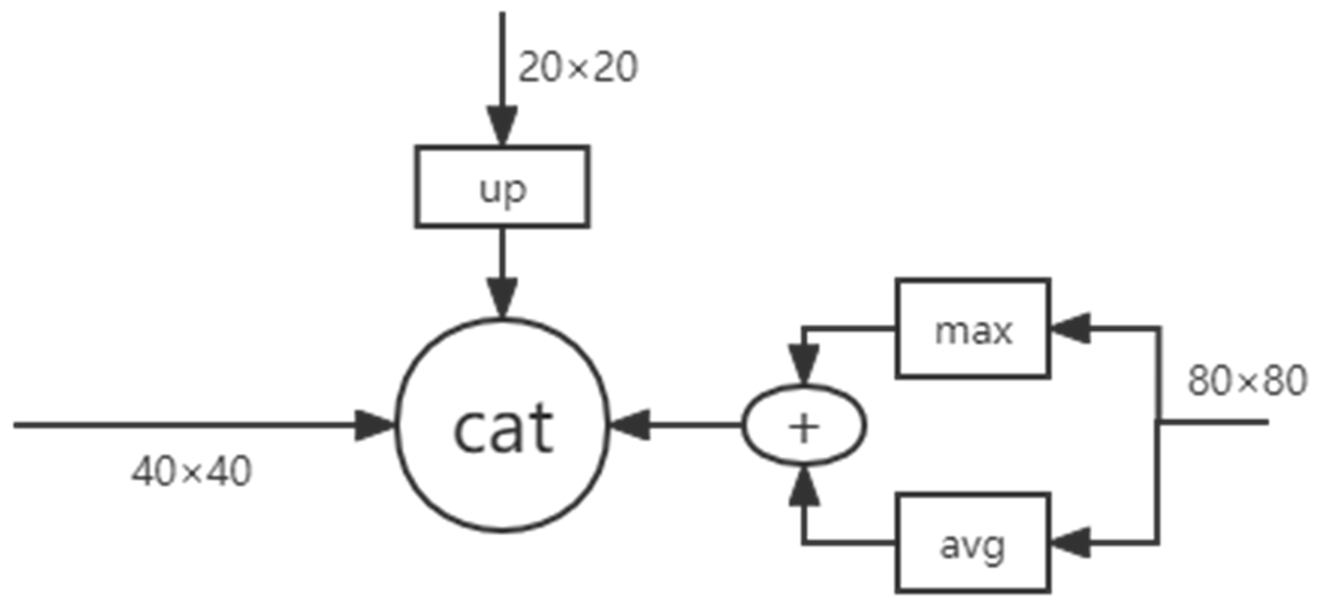
3.1.1. Multicat Module
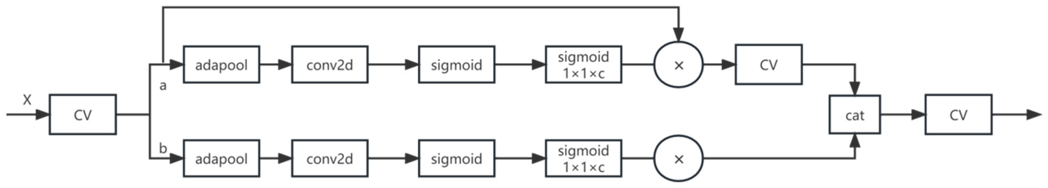
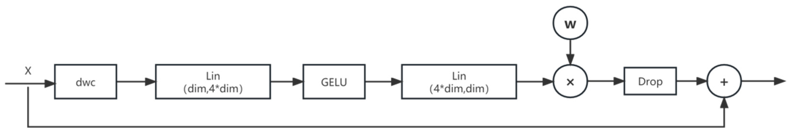
3.1.2. Mc2f Module
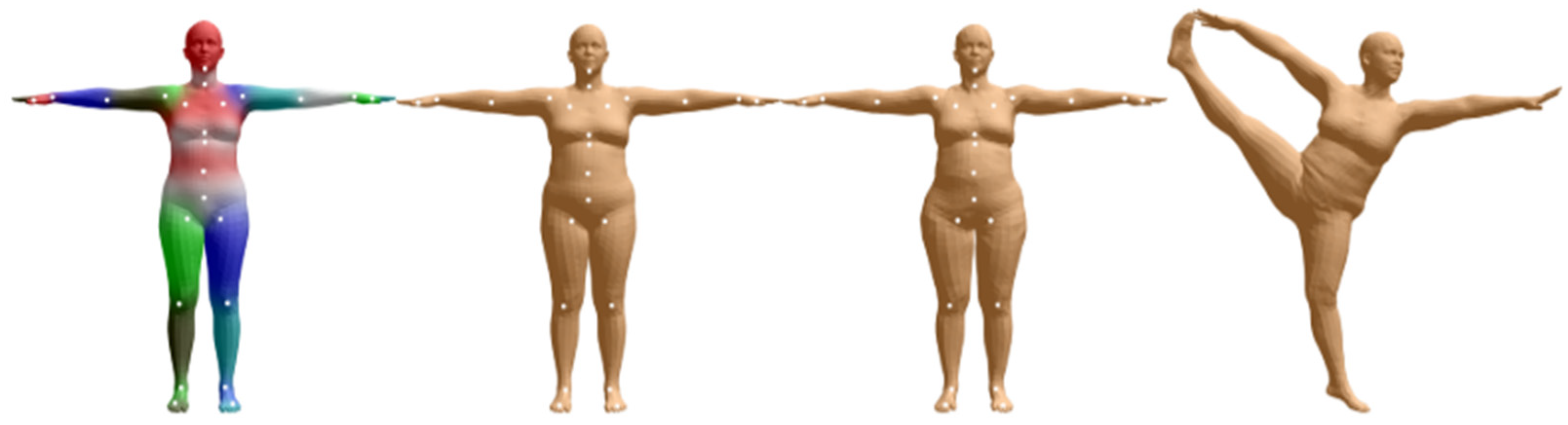
3.2. Joint Angle Calculation and Pcf Fitting
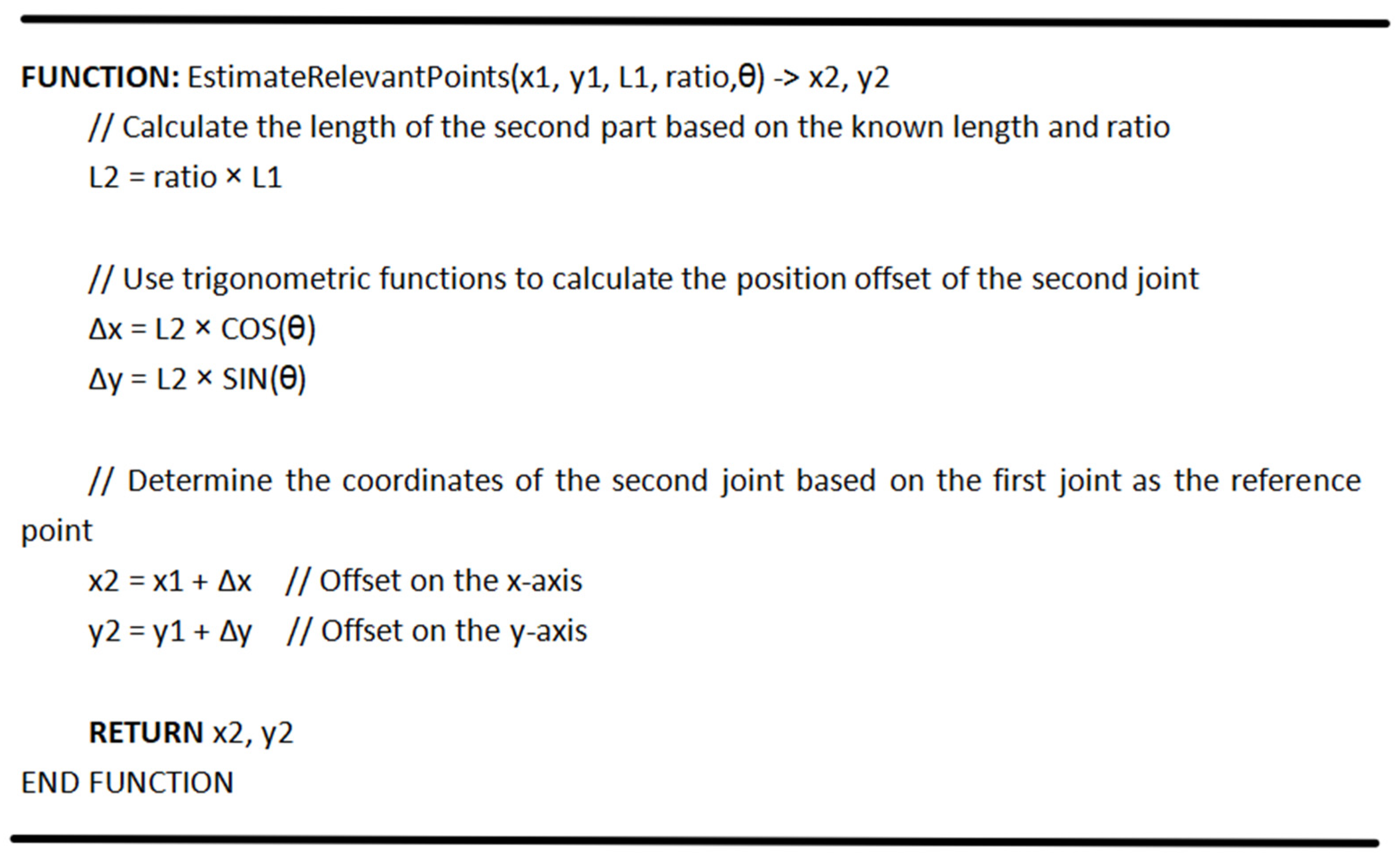
3.2.1. Joint Angle Calculation
3.2.2. Polynomial Fitting Correction
3.2.3. Evaluation Metrics for Fitting Corrections to Joint Angles
- (1)
- Leakage rate
- (2)
- Error detection rate
4. Experiments and Results
4.1. Datasets
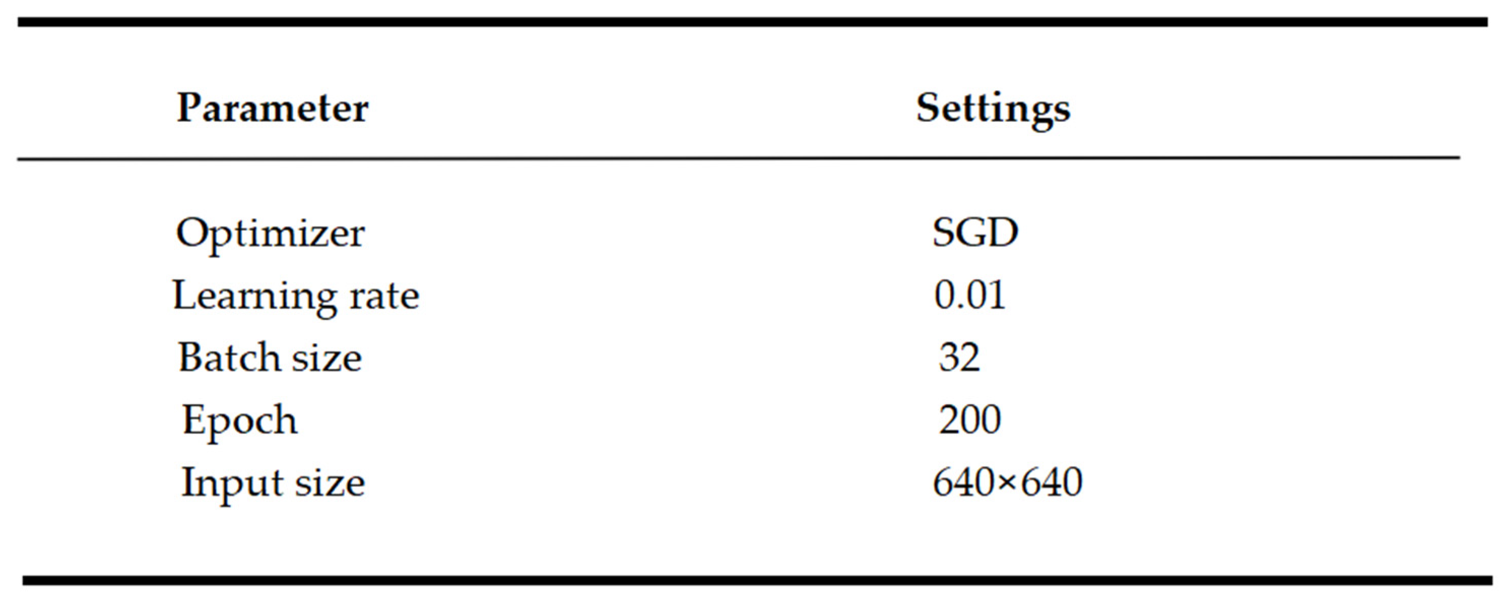
4.2. Yolov8-sp Training Details
4.3. Comparison of Models
4.3.1. Comparison of Baseline Models
4.3.2. Comparison with Advanced Models
4.3.3. Comparison with Openpose
4.4. Polynomial Fitting of Joint Angles
4.4.1. Quantitative Evaluation
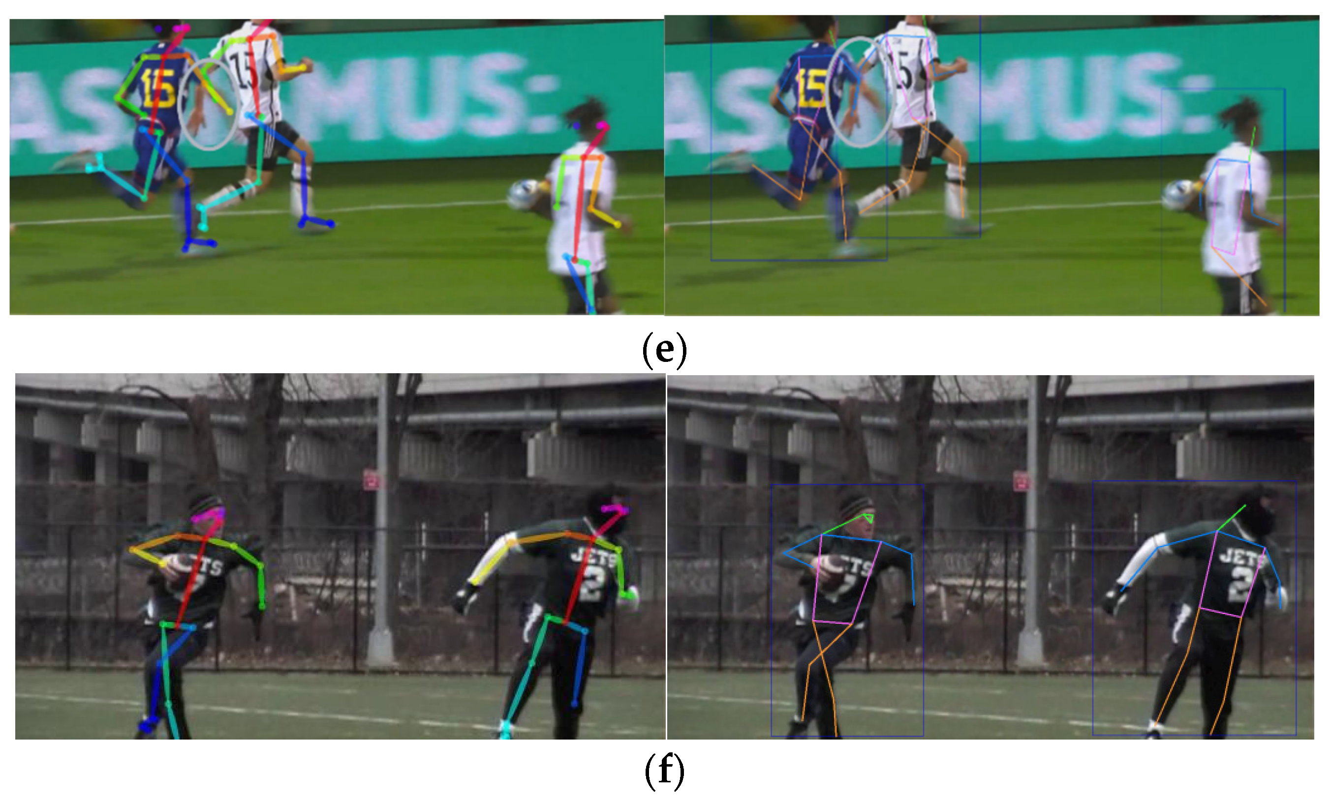
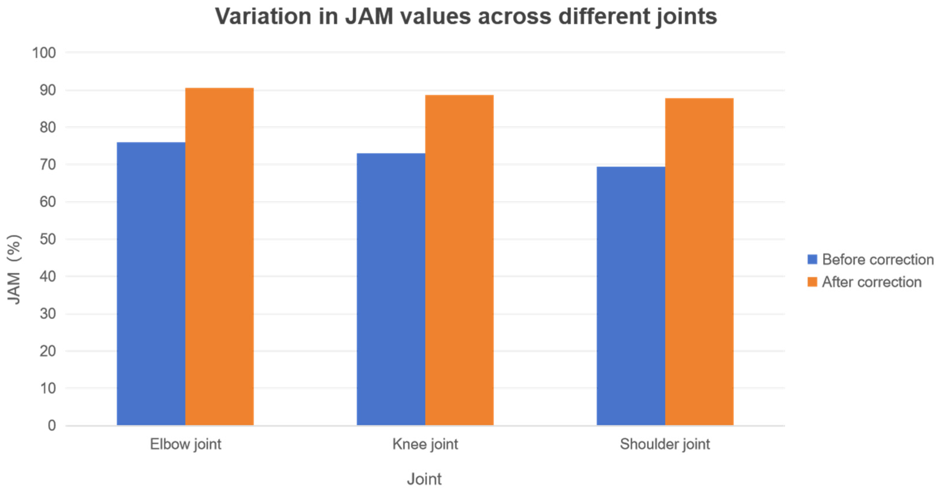
4.4.2. Qualitative Assessment of Joint Angles
5. Conclusions
Author Contributions
Funding
Data Availability Statement
Acknowledgments
Conflicts of Interest
References
- He, K.; Gkioxari, G.; Dollár, P.; Girshick, R. Mask R-CNN. In Proceedings of the IEEE International Conference on Computer Vision, Venice, Italy, 22–29 October 2017; pp. 2961–2969. [Google Scholar]
- Chen, Y.; Wang, Z.; Peng, Y.; Zhang, Z.; Yu, G.; Sun, J. Cascaded Pyramid Network for Multi-Person Pose Estimation. In Proceedings of the IEEE Conference on Computer Vision and Pattern Recognition, Salt Lake City, UT, USA, 18–23 June 2018; pp. 7103–7112. [Google Scholar]
- Tian, Z.; Chen, H.; Shen, C. DirectPose: Direct End-to-End Multi-Person Pose Estimation. arXiv 2019, arXiv:1911.07451. [Google Scholar]
- Sun, K.; Xiao, B.; Liu, D.; Wang, J. Deep High-Resolution Representation Learning for Human Pose Estimation. In Proceedings of the IEEE/CVF Conference on Computer Vision and Pattern Recognition, Long Beach, CA, USA, 15–20 June 2019; pp. 5693–5703. [Google Scholar]
- Xiao, B.; Wu, H.; Wei, Y. Simple Baselines for Human Pose Estimation and Tracking. In ECCV; Springer: Berlin/Heidelberg, Germany, 2018. [Google Scholar]
- Ke, L.; Chang, M.-C.; Qi, H.; Lyu, S. DetposeNet: Improving Multi-Person Pose Estimation via Coarse-Pose Filtering. IEEE Trans. Image Process 2022, 31, 2782–2795. [Google Scholar] [CrossRef] [PubMed]
- Lee, J.; Kim, T.-y.; Beak, S.; Moon, Y.; Jeong, J. Real-Time Pose Estimation Based on ResNet-50 for Rapid Safety Prevention and Accident Detection for Field Workers. Electronics 2023, 12, 3513. [Google Scholar] [CrossRef]
- Cao, Z.; Simon, T.; Wei, S.-E.; Sheikh, Y. Realtime multi-person 2D pose estimation using part affinity fields. In Proceedings of the IEEE Conference on Computer Vision and Pattern Recognition, Honolulu, HI, USA, 21–26 July 2017; pp. 7291–7299. [Google Scholar]
- Wei, S.-E.; Ramakrishna, V.; Kanade, T.; Sheikh, Y. Convolutional Pose Machines. In Proceedings of the IEEE Conference on Computer Vision and Pattern Recognition, Las Vegas, NV, USA, 27–30 June 2016; pp. 4724–4732. [Google Scholar]
- Kocabas, M.; Karagoz, S.; Akbas, E. MultiPoseNet: Fast Multi-Person Pose Estimation Using Pose Residual Network. In Proceedings of the European Conference on Computer Vision (ECCV), Munich, Germany, 8–14 September 2018; pp. 417–433. [Google Scholar]
- Geng, Z.; Sun, K.; Xiao, B.; Zhang, Z.; Wang, J. Bottom-Up Human Pose Estimation via Disentangled Keypoint Regression. In Proceedings of the IEEE/CVF Conference on Computer Vision and Pattern Recognition, Nashville, TN, USA, 20–25 June 2021; pp. 14676–14686. [Google Scholar]
- Brasó, G.; Kister, N.; Leal-Taixé, L. The Center of Attention: Center-Keypoint Grouping via Attention for Multi-Person Pose Estimation. In Proceedings of the IEEE/CVF International Conference on Computer Vision, Montreal, QC, Canada, 10–17 October 2021; pp. 11853–11863. [Google Scholar]
- Wang, D.; Zhang, S.; Hua, G. Robust Pose Estimation in Crowded Scenes with Direct Pose-Level Inference. Adv. Neural Inf. Process. Syst. 2021, 34, 6278–6289. [Google Scholar]
- Wang, L.; Su, B.; Liu, Q.; Gao, R.; Zhang, J.; Wang, G. Human Action Recognition Based on Skeleton Information and Multi-Feature Fusion. Electronics 2023, 12, 3702. [Google Scholar] [CrossRef]
- Wu, C.; Wei, X.; Li, S.; Zhan, A. MSTPose: Learning-Enriched Visual Information with Multi-Scale Transformers for Human Pose Estimation. Electronics 2023, 12, 3244. [Google Scholar] [CrossRef]
- Hendrycks, D.; Gimpel, K. Gaussian Error Linear Units (GELUs). arXiv 2016, arXiv:1606.08415. [Google Scholar]
- Glenn, J. Ultralytics YOLOv8. 2023. Available online: https://github.com/ultralytics/ultralytics (accessed on 2 March 2023).
- He, K.; Zhang, X.; Ren, S.; Sun, J. Deep Residual Learning for Image Recognition. In Proceedings of the IEEE Conference on Computer Vision and Pattern Recognition, Las Vegas, NV, USA, 27–30 June 2016; pp. 770–778. [Google Scholar]
- Maji, D.; Nagori, S.; Mathew, M.; Poddar, D. YOLO-Pose: Enhancing YOLO for Multi-Person Pose Estimation Using Object Keypoint Similarity Loss. arXiv 2022, arXiv:2204.06806. [Google Scholar] [CrossRef]
- Nair, V.; Hinton, G.E. Rectified Linear Units Improve Restricted Boltzmann Machines. In Proceedings of the 27th International Conference on International Conference on Machine Learning, Haifa, Israel, 21–24 June 2010. [Google Scholar]
- Loper, M.; Mahmood, N.; Romero, J.; Pons-Moll, G.; Black, M.J. SMPL: A Skinned Multi-Person Linear Model. ACM Trans. Graph. 2015, 34, 248. [Google Scholar] [CrossRef]
- Lin, T.Y.; Dollár Piotr Girshick, R.; He, K.; Hariharan, B.; Belongie, S. Feature Pyramid Networks for Object Detection. In Proceedings of the 2017 IEEE Conference on Computer Vision and Pattern Recognition (CVPR), Honolulu, HI, USA, 21–26 July 2017. [Google Scholar]
- Liu, Z.; Mao, H.; Wu, C.Y.; Feichtenhofer, C.; Darrell, T.; Xie, S. A ConvNet for the 2020s. arXiv 2022, arXiv:2201.03545. [Google Scholar]
- Devlin, J.; Chang, M.-W.; Lee, K.; Toutanova, K. BERT: Pre-training of Deep Bidirectional Transformers for Language Understanding. In Proceedings of the 2019 Conference of the North American Chapter of the Association for Computational Linguistics: Human Language Technologies, Minneapolis, MN, USA, 3–5 June 2019. [Google Scholar]
- Radford, A.; Wu, J.; Child, R.; Luan, D.; Amodei, D.; Sutskever, I. Language Models Are Unsupervised Multitask Learners. J. OpenAI 2019, 1, 8. [Google Scholar]
- Vaswani, A.; Shazeer, N.; Parmar, N.; Uszkoreit, J.; Jones, L.; Gomez, A.N.; Kaiser, L. Attention is all you need. Adv. Neural Inf. Process. Syst. 2017, 30, 5998–6008. [Google Scholar]
- Hu, H.; Zhang, Z.; Xie, Z.; Lin, S. Local relation networks for image recognition. In Proceedings of the IEEE/CVF International Conference on Computer Vision (ICCV), Seoul, Republic of Korea, 27 October 2019–2 November 2019; pp. 3464–3473. [Google Scholar]
- Veit, A.; Wilber, M.J.; Belongie, S. Residual networks behave like ensembles of relatively shallow networks. In Proceedings of the Advances in Neural Information Processing Systems, Barcelona, Spain, 5–10 December 2016. [Google Scholar]
- Cheng, B.; Xiao, B.; Wang, J.; Shi, H.; Huang, T.S.; Zhang, L. HigherHRNet: Scale-Aware Representation Learning for Bottom-Up Human Pose Estimation. In Proceedings of the IEEE/CVF Conference on Computer Vision and Pattern Recognition (CVPR), Seattle, WA, USA, 14–19 June 2020. [Google Scholar]
- Redmon, J.; Divvala, S.; Girshick, R. You Only Look Once: Unified, Real-Time Object Detection. In Proceedings of the 2016 IEEE Conference on Computer Vision and Pattern Recognition (CVPR), Las Vegas, NV, USA, 27–30 June 2016; pp. 779–788. [Google Scholar]
- Newell, A.; Yang, K.; Deng, J. Stacked Hourglass Networks for Human Pose Estimation. arXiv 2016, arXiv:1603.06937. [Google Scholar]
- Osokin, D. Real-time 2D Multi-Person Pose Estimation on CPU: Lightweight OpenPose. arXiv 2018, arXiv:1811.12004. [Google Scholar]


| Joints | Left | Right |
|---|---|---|
| Elbow joint | 5–6–7 | 2–3–4 |
| Knee joint | 11–12–13 | 8–9–10 |
| Shoulder joint | 1–5–6 | 1–2–3 |
| Method | Multicat | mc2f | ||||
|---|---|---|---|---|---|---|
| (1) | 85.4 | 59.5 | 60.7 | 74.3 | ||
| (2) | √ | 86.4 | 60.1 | 61.6 | 75.6 | |
| (3) | √ | 86.9 | 60.7 | 62.0 | 74.4 | |
| (4) | √ | √ | 87.1 | 61.9 | 61.8 | 75.9 |
| Methods | Backbone | ||||
|---|---|---|---|---|---|
| HRnet [4] | HRnet-W32 | 84.0 | 52.6 | 58.3 | 72.7 |
| HigherHRNnet [29] | HRnet-W48 | 84.6 | 53.2 | 58.4 | 73.1 |
| Yolov5pose [30] | Darknet-csp-d53-s | 85.2 | 58.4 | 58.7 | 73.5 |
| Openpose [8] | ------------- | 83.3 | 53.9 | 57.4 | 71.9 |
| Hourglass [31] | Hourglass | 82.9 | 52.6 | 56.1 | 69.2 |
| Lightopenpose [32] | ------------- | 78.5 | 51.3 | 55.8 | 67.7 |
| Ours | Darknet-53 | 87.1 | 60.8 | 61.8 | 75.9 |
| Type | ||||||
|---|---|---|---|---|---|---|
| Tennis | 90.5 | 88.2 | 87.0 | 10.4 | 11.6 | 14.6 |
| Football | 86.1 | 84.4 | 80.2 | 16.7 | 15.5 | 17.3 |
| Skiing | 88.4 | 88.3 | 89.5 | 16.3 | 14.1 | 13.8 |
| Gymnastics | 95.5 | 94.0 | 93.6 | 11.3 | 10.2 | 13.4 |
| Running | 92.3 | 88.7 | 88.9 | 12.9 | 13.9 | 18.6 |
Disclaimer/Publisher’s Note: The statements, opinions and data contained in all publications are solely those of the individual author(s) and contributor(s) and not of MDPI and/or the editor(s). MDPI and/or the editor(s) disclaim responsibility for any injury to people or property resulting from any ideas, methods, instructions or products referred to in the content. |
© 2023 by the authors. Licensee MDPI, Basel, Switzerland. This article is an open access article distributed under the terms and conditions of the Creative Commons Attribution (CC BY) license (https://creativecommons.org/licenses/by/4.0/).
Share and Cite
Wang, S.; Zhang, X.; Ma, F.; Li, J.; Huang, Y. Single-Stage Pose Estimation and Joint Angle Extraction Method for Moving Human Body. Electronics 2023, 12, 4644. https://doi.org/10.3390/electronics12224644
Wang S, Zhang X, Ma F, Li J, Huang Y. Single-Stage Pose Estimation and Joint Angle Extraction Method for Moving Human Body. Electronics. 2023; 12(22):4644. https://doi.org/10.3390/electronics12224644
Chicago/Turabian StyleWang, Shuxian, Xiaoxun Zhang, Fang Ma, Jiaming Li, and Yuanyou Huang. 2023. "Single-Stage Pose Estimation and Joint Angle Extraction Method for Moving Human Body" Electronics 12, no. 22: 4644. https://doi.org/10.3390/electronics12224644
APA StyleWang, S., Zhang, X., Ma, F., Li, J., & Huang, Y. (2023). Single-Stage Pose Estimation and Joint Angle Extraction Method for Moving Human Body. Electronics, 12(22), 4644. https://doi.org/10.3390/electronics12224644