Article

Human Body as a Signal Transmission Medium for Body-Coupled Communication: Galvanic-Mode Models

Institute of Electronics and Computer Science (EDI), Dzerbenes 14, LV-1006 Riga, Latvia
*
Author to whom correspondence should be addressed.
Electronics 2023, 12(21), 4550; https://doi.org/10.3390/electronics12214550
Submission received: 11 October 2023 / Revised: 1 November 2023 / Accepted: 3 November 2023 / Published: 6 November 2023

Abstract

:
Signal propagation models play a fundamental role in radio frequency communication research. However, emerging communication methods, such as body-coupled communication (BCC), require the creation of new models. In this paper, we introduce mathematical models that approximate the human body as an electrical circuit, as well as linear regression- and random forest-based predictive models that infer the expected signal loss from its frequency, measurement point locations, and body parameters. The results demonstrate a close correspondence between the amplitude-frequency response (AFR) predicted by the electrical circuit models and the experimental data gathered from volunteers. The accuracy of our predictive models was assessed by using their root mean square errors (RMSE), ranging from 1.5 to 7 dB depending on the signal frequency within the 0.05 to 20 MHz range. These results allow researchers and engineers to simulate and forecast the expected signal loss within BCC systems during their design phase.

1. Introduction

The development of microelectronics has facilitated the placement of sensors on the human body to create body-area networks (BANs). These networks serve as valuable data sources for healthcare and fitness applications. Signals from on-body sensors are collected and processed to derive clinically relevant information. Typically, this data collection is carried out by a smartwatch or a device connected to a smartwatch, such as a mobile phone, cloud server, or edge server. However, the transmission of potentially sensitive data from on-body sensors to the collector device raises security concerns. Traditional options like Bluetooth and WiFi are vulnerable to security threats and side-channel attacks via signal interception. Body-coupled communication (BCC) emerges as a novel communication technology that utilizes the human body for data transfer. Unlike traditional methods, BCC eliminates data transmission over the air, significantly reducing the risk of security breaches. This is particularly important for health-related data, given their stringent privacy and authenticity requirements.
BCC uses low-voltage AC as the carrier wave, typically in frequencies up to 100 MHz. This frequency range experiences lower signal attenuation within the human body compared with radio frequency signals. Consequently, BCC systems hold the potential to be an order of magnitude more efficient than their conventional wireless counterparts [1]. However, the specific characteristics of the human body as a transmission medium for BCC signals remain incompletely understood. This is especially the case for galvanic (“voltage mode”) BCC, where two pairs of electrodes are connected to the human body, and both the forward and backward signal propagation paths go through the human body. In order to address this knowledge gap, this paper utilizes a galvanic BCC dataset collected from 30 volunteers [2]. The dataset includes frequencies ranging from 0.05 to 20 MHz and is described in more detail in [3].
Our first approach is to model the BCC system, including the human body, with electrical circuits. Here, the objectives are (1) to derive operator transfer functions from the proposed circuit models, subsequently allowing us to obtain amplitude-frequency responses (AFRs) for these models, and (2) to establish nominal values for the circuit components in a manner that closely aligns the AFR of the model with experimental data.
Our second approach is to use statistics and machine learning to design predictive models capable of estimating signal loss in BCC communication links. These models utilize signal frequency, transmitter and receiver locations, and human body properties as input parameters. We anticipate that these predictive models will find valuable applications, for instance, to help create accurate BCC system simulators [4] and allow practitioners to determine the minimum requirements and constraints for real BCC systems during their design phase. To the best of our knowledge, we are the first to present BCC models of this type. The feasibility of accurate statistical models is contingent on the availability of a substantial experimental dataset, which was made possible through the collection of the BCC measurement dataset available at [2].
Our main contributions are the following:
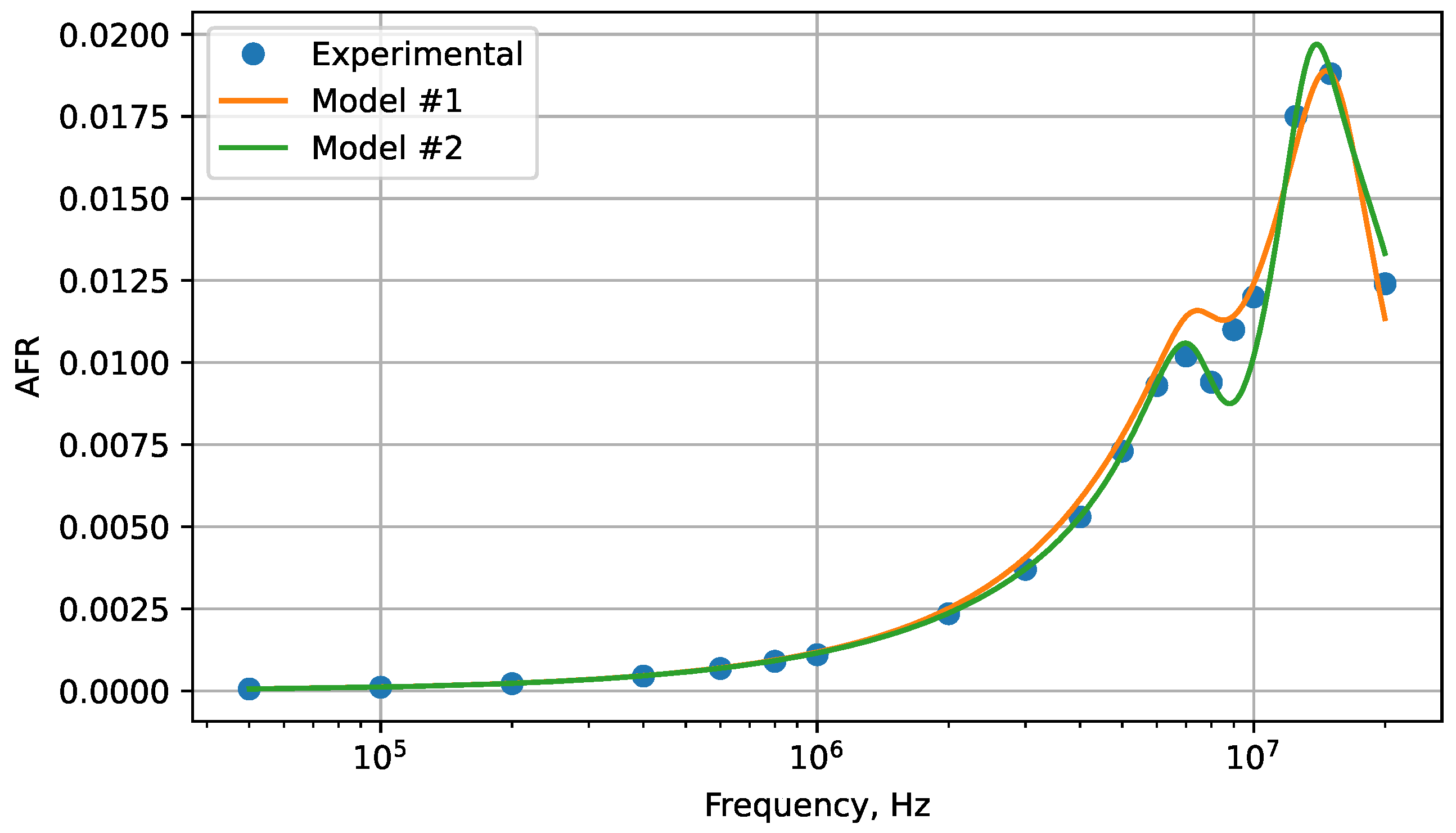
  • Present two electrical circuit models of a BCC system: one adapted from existing work (Model #1) and another that is simpler but similarly accurate (Model #2);
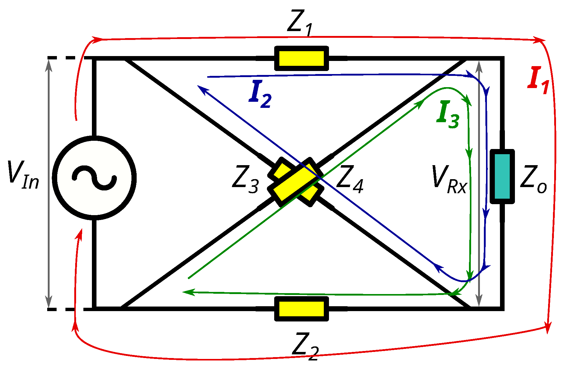
  • Provide closed-form expressions of the transfer function in both circuit models;
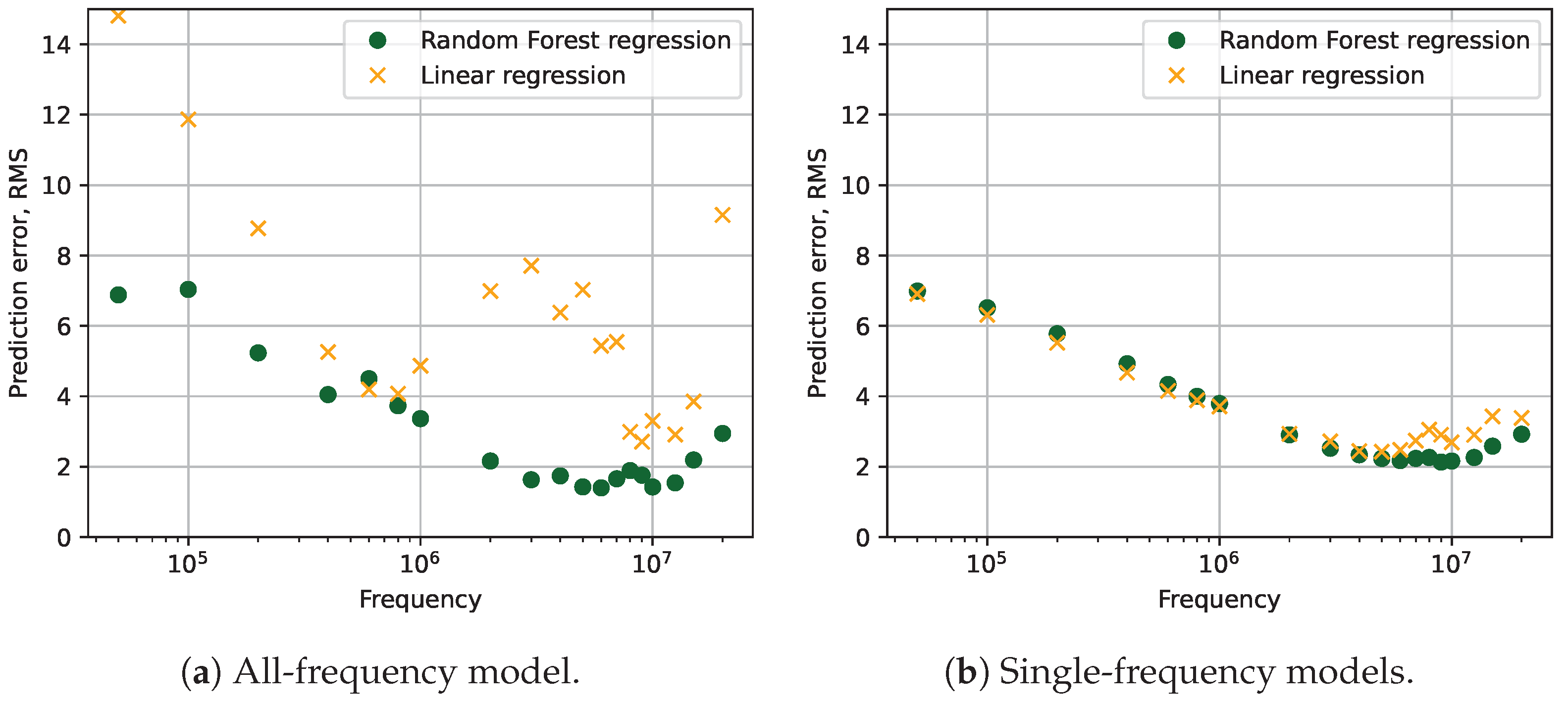
  • Apply linear regression and random forest regression methods to construct and evaluate multiple predictive models.
This work uses materials from the extended abstract [5] presented at the International Workshop on Embedded Digital Intelligence (IWoEDI’2023). Specifically, Model #2 in the current article is taken from this source. The present article adds the description and experimental results of Model #1, additional experimental results for #2, and the linear regression and random forest regression-based predictive models (Section 4), as well as a review of the related work on this topic.

2. Related Work

BCC as a field was established over three decades ago with the pioneering work of Wegmueller et al. [6]. While BCC remains at a relatively low technology readiness level (TRL), this technology has attributes that render it competitive against more established communication protocols such as Bluetooth and WiFi. BCC is considered especially suitable for the transmission of health-related data. This is due to its inherent security features (minimized signal leakage) and its ability to operate at low transmission power levels, thanks to the lower attenuation of lower-frequency BCC signals when passing through the human body, compared with radio frequency signals [7,8]. The main application of BCC is in the construction of wireless body area networks [9]. The BCC-enabled devices can transmit on-body or intrabody sensor data while only consuming a few μ W of power [10].
The existing literature differs at the level at which the human body is modeled. Some works treat the human body as a black box, representing it as a single element with complex resistance [11]. In taking a step further, others model the forward and return paths as separate impedances [12], while some incorporate interpath elements into the circuit model [7,13,14]. The most comprehensive work using this approach so far is by Modak et al. [15]. Their model includes the impedances of skin and muscles and the impacts of the external (ground) couplings. Their results show that signal loss increases gradually for short distances but converges to a fixed value for distances much further than the separation distance between the contact electrode pairs.
When pushing towards higher levels of detail, some studies use different kinds of models, such as finite element models [13,16,17]. Song et al. [13] provided a simplified 3D model of the human body and used it in finite-element simulations, demonstrating a good match between the simulation and experimental results. Park et al. [16] presented another hybrid electrostatic finite element model and demonstrated measurement-to-simulation agreement within 2.5 dB. Ito et al. [17] focused on modeling a human arm with the help of a finite element model.
Besides the capacitive and galvanic BCC usually presented in the research literature, there are other modes. For instance, more recent work has started to investigate magnetic human-body communication (mHBC). Wen et al. [18] provide a radiating near-field coupling model and numerical simulations to demonstrate that magnetic communication minimizes channel loss at the 100–200 MHz frequency band. Moreover, radio frequency signals can also be used to communicate through the human body. Asan et al. [19] used numerical and ex vivo models to show that the intrabody fat tissue has good radio signal propagation characteristics and can be used to send radio waves deep into the human body without large absorption losses, whereas crossing a single blood vessel can cause up to a 17.1 dB signal loss. Demir et al. [20] created RF signal propagation models from data obtained from a human cadaver. Last but not least, ultrasound is another promising way of achieving intrabody communication and comes with its own models. Jiang et al. [21] presented an early-stage modeling work that uses simple geometric models for ultrasound propagation. They derive the channel impulse response and other properties under these simplified assumptions.
In our research, we build upon an electrical circuit model described in the survey paper of Song et al. [13], instantiating it and evaluating its performance, as well as introducing a new version with lower complexity and similar numerical accuracy. Furthermore, to the best of our knowledge, our work pioneers the application of statistical and machine-learning techniques in this domain.
The adoption of statistical and machine learning approaches in our research is made possible by our novel dataset [2]. As demonstrated in prior studies [22,23], existing empirical BCC measurement studies suffer from setup issues and ambiguities surrounding measurement parameters. The dataset used in this work aims to avoid these problems and is collected using state-of-the-art methods [3]. Notably, the signal loss curves within our dataset closely align with results found in the existing literature that employ similar experimental setups [12,22,23].

3. Electrical Circuit Models

3.1. Problem Formulation

Consider the human body as a signal transmission medium between two pairs of electrodes. The goal of a BCC system is to transmit a modulated carrier wave from the transmitter (Tx) side to the receiver (Rx) side electrodes. A BCC system features a generator with internal resistance R g that generates an electrical sine wave and a receiver—an oscilloscope or a similar detector—with internal impedance Z o .
Low signal loss between the Tx and Rx is a desirable property of such a system as it allows the following:
  • Makes the system more energy-efficient and alleviates any health-related concerns by minimizing the electric current that enters the human body;
  • Reduces the sophistication required from the detector on the Rx side, as higher amplitude signals are easier to register and decode without errors.
The dataset [2] follows the convention in BCC that typically defines the signal loss in the system in terms of a voltage drop between the sender and the receiver [23]. Although some works do use power loss [22], it is more difficult to experimentally measure it with high accuracy since power loss depends on whether the impedance is matched in the system. In order to minimize the impact of the system itself on the measurement results if power loss is measured, impedance matching or table-based correction is required. Therefore, it is not practical to collect large, accurate datasets with power loss as the metric since every human, every pair of Rx and Tx points, and every frequency has a different impedance.
The signal loss in a BCC system depends both on the properties of the human body and the setup of the system itself. System parameters, such as generator output resistance, R g , and receiver input resistance, Z o , are determined by the choice of the devices and can take different values in different systems. Along with the generator voltage, the values of R g and Z o determine the current through the human body and the voltage drop over it. As a result, the communication system needs to be modeled as a whole, with the human body as a part of that system.
The voltage drop at a fixed signal frequency is defined as the ratio of the input voltage to the output voltage at that frequency. This ratio is often expressed in decibels. For the purposes of modeling, it is more conventional to refer to the amplitude-frequency response (AFR) of the system—an alternative but equivalent way to treat voltage drop. For a fixed frequency, f, the AFR is described by a scalar variable, K, such that K · V T x = V R x .
Our approach takes the following form:
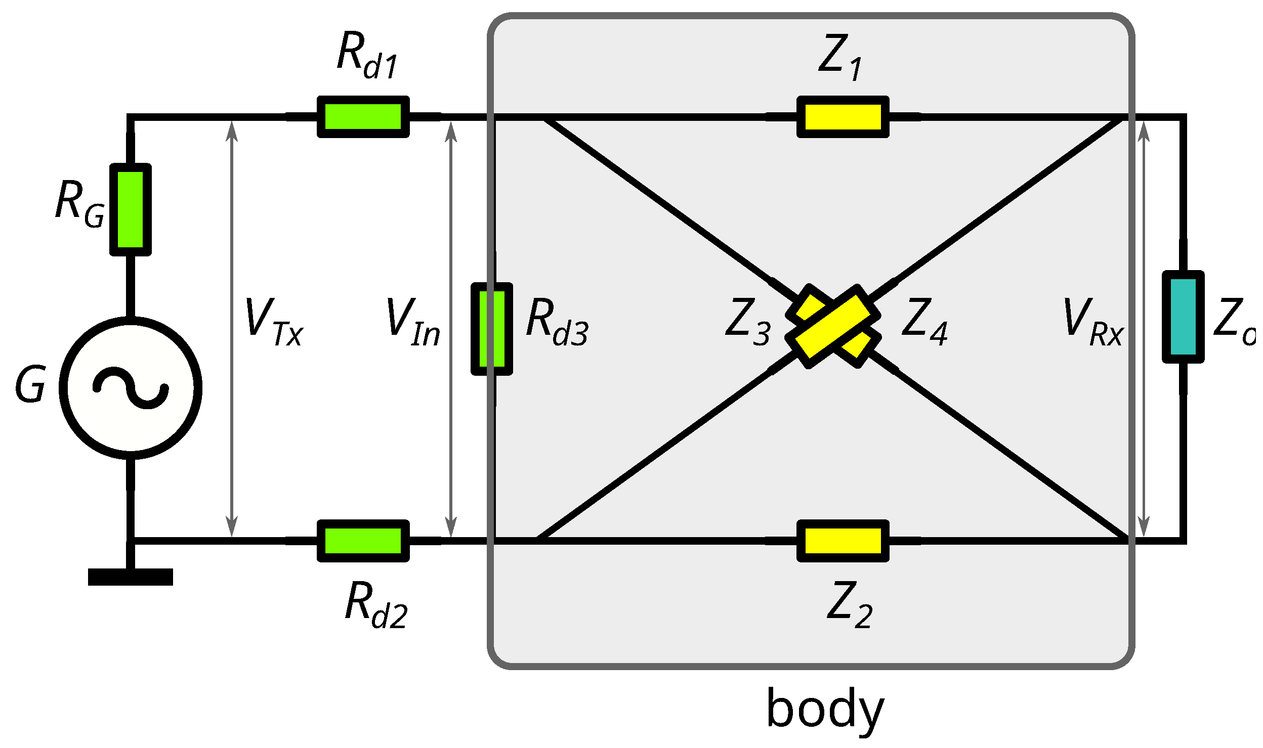
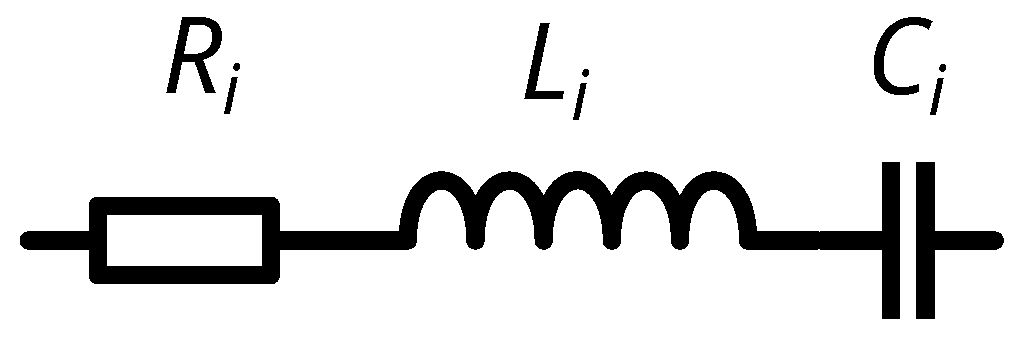
  • Provide circuit models (Figure 1 and Figure 4) of the communication system that include the human body and the BCC equipment;
  • Simplify and divide the models into parts to make it tractable to express the AFR with closed-form algebraic equations;
  • Find nominal values of the components in the models using experimental AFR data as the ground truth.

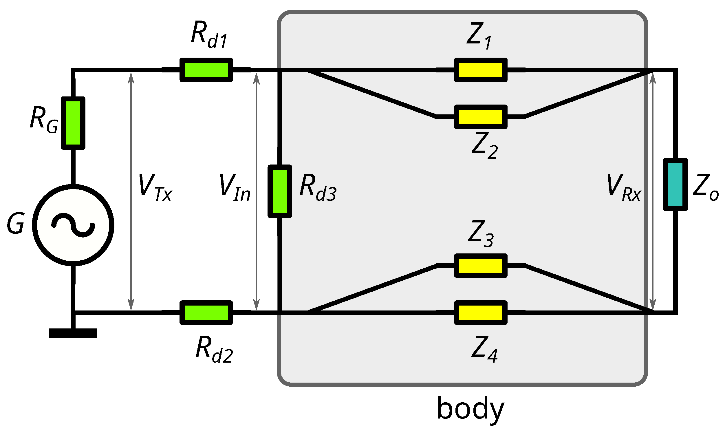
3.2. Circuit Model #1

The first model (Figure 1) is a modified version of the model proposed in [13]. The following components are present in the model:
  • G and R G — signal generator and its internal resistance;
  • R d 1 , d 2 , d 3 — resistances related to electrode and skin contacts;
  • Z o — the entry impedance of the signal detector;
  • Z 1 , 2 , 3 , 4 — impedances between the receiver and transmitter electrodes.
The components, R d i , refer to the cumulative resistance values on both sides of the body for the Tx and Rx-side electrodes.
The analysis of the model can be made more tractable by separating it in two parts: the left and the right side. The left side of the model includes the divider resistances R d 1 , R d 2 , R d 3 that describe the electrode-skin coupling [13]. As the resistances R d i are much smaller than the absolute values of the impedances, Z i , it is possible to simplify the algebraic expression of the voltage gain with very little loss of accuracy by replacing the generator voltage, V T x , and the divider resistances, R d i , with an equivalent generator with a voltage, V I n , and a small internal resistance, R g , so that
K = V I n V T x · V R x V I n
Let us denote the first ratio with K l e f t and the second ratio with K r i g h t and analyze them separately. The left side of the model is simple to analyze:
K l e f t = R d 3 R d 1 + R d 2 + R d 3
Finding an analytic expression for the right side is the main task of the subsequent analysis.
The right side of the model (Figure 2) includes a circuit consisting of complex resistances Z 1 , Z 2 , Z 3 , Z 4 . In order to find K r i g h t , we use Kirchhoff’s second law to make the following system of equations for circuit currents I 1 , I 2 , I 3 (Figure 2):
Z 1 ( I 1 + I 2 ) + Z o ( I 1 + I 2 + I 3 ) + Z 2 ( I 1 + I 3 ) = V I n
Z 1 ( I 1 + I 2 ) + Z o ( I 1 + I 2 + I 3 ) + Z 4 I 2 = 0
Z 3 I 3 + Z o ( I 1 + I 2 + I 3 ) + Z 2 ( I 1 + I 3 ) = 0
By solving this system of equations, we find the currents, I i , and from them, the voltage at the receiver, V R x . Dividing V R x by the input voltage V I n results in K r i g h t , by definition. It equals
K r i g h t = Z o ( Z 3 Z 4 Z 1 Z 2 ) Z o ( Z 2 Z 3 + Z 1 Z 4 + Z 1 Z 2 + Z 3 Z 4 ) + Z 1 Z 2 ( Z 3 + Z 4 ) + Z 3 Z 4 ( Z 1 + Z 2 )
Each of the impedances, Z i , can be modeled as series of R , L , C (resistance, inductance, and capacitance) elements (Figure 3):
Z i = R i + 2 j π f L i + 1 j 2 π f C i
where f is the frequency of the signal.
In most of the models described in the existing literature, the human body is represented as an R C circuit; the inductive (L) elements are typically not included (one exception is Ito et al. [17]). However, Our models (Figure 1 and Figure 4) do include L elements. As shown in Figure 5 and Figure 6, the experimentally obtained AFR curve of the human body has two pronounced resonance peaks in the 0.05 to 20 MHz frequency band that we investigated. It is not natural to obtain such large resonances using only R C elements; therefore, we achieve them by using R L C circuits in the model.
Let us now define the transfer function K ( f ) such that the desired AFR K at a specific frequency, f, is equal to the absolute value of K ( f ) :
K = | K ( f ) |
The next step is to replace j 2 π f with a complex variable, p, in order to simplify the expressions ( K ( p ) = K ( f ) ):
p : = j 2 π f
By combining Equations (2) and (6), replacing Z i with the series of elements and simplifying the result, we obtain a formula for the transfer function K ( p ) :
K ( p ) = K o a p 5 + b p 4 + c p 3 + d p 2 + e p h p 6 + i p 5 + k p 4 + g p 3 + m p 2 + n p + q ,
where
K o = Z o R d 3 a = C 1 C 2 C 3 C 4 ( L 3 L 4 L 1 L 2 ) b = C 1 C 2 C 3 C 4 ( L 3 R 4 + L 4 R 3 L 2 R 1 L 1 R 2 ) c = C 1 C 2 C 3 C 4 ( R 3 R 4 R 1 R 2 ) + C 1 C 2 ( L 3 C 3 ) C 3 C 4 ( L 2 C 2 L 1 C 1 ) d = C 1 C 2 ( R 3 C 3 + R 4 C 4 ) C 3 C 4 ( R 2 C 2 + R 1 C 1 ) e = C 1 C 2 C 1 C 2
The coefficients in the denominator are an order of magnitude more cumbersome expressions; therefore, we only include the full K ( p ) expression in the Supplementary Materials.

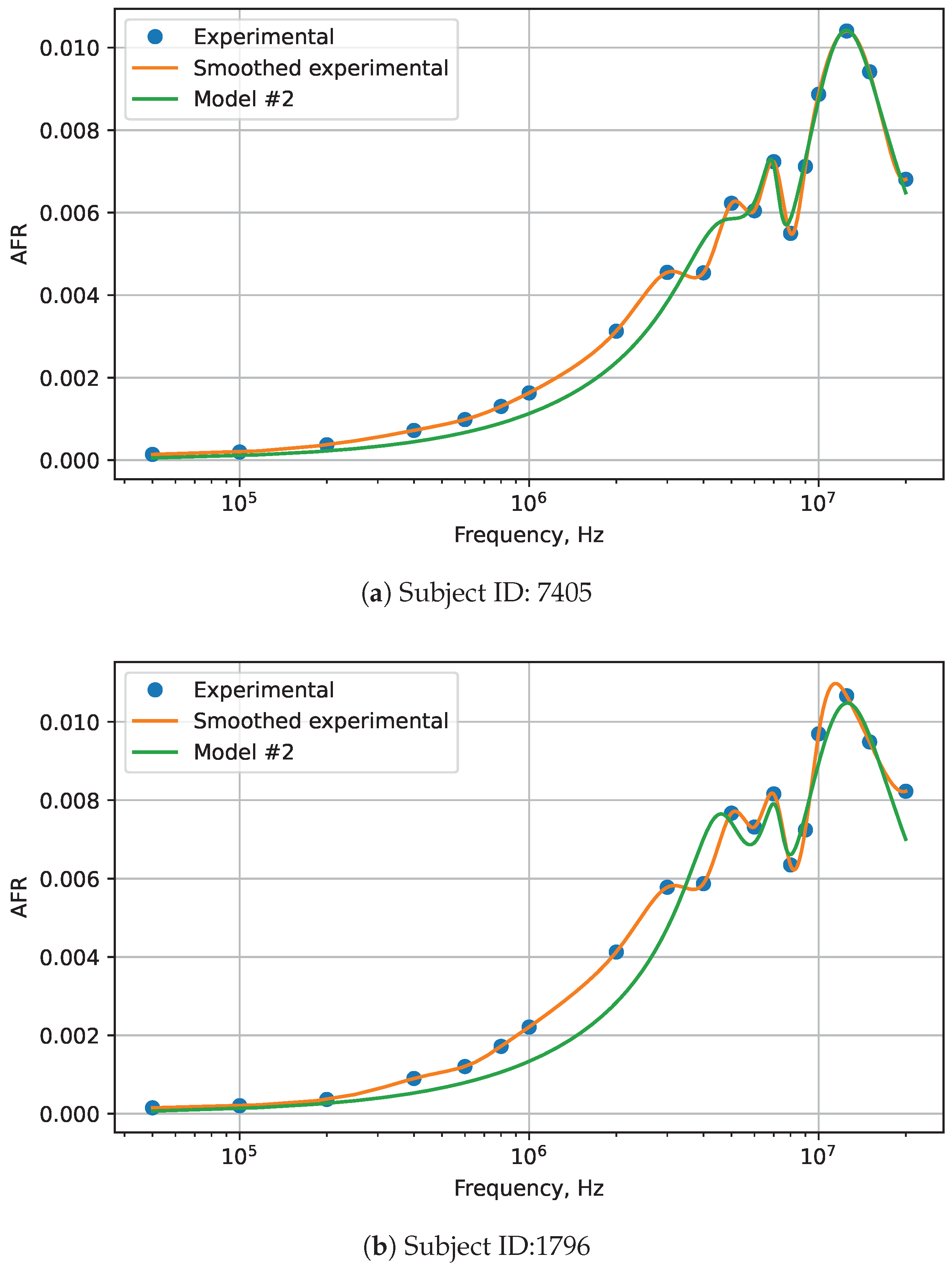
3.3. Circuit Model #2

Model #1 produces a good overall approximation of real-world characteristics, notably the AFR, as shown later in Section 3.4. However, it has a limitation, namely, that each of the Z i elements in the circuit exerts a significant influence on the entire AFR profile since they are connected diagonally. Given the distinctive AFR characteristics anticipated, featuring two closely spaced resonances, we present a second model (Figure 4) that closely aligns with these requirements and differs from the previous one by eliminating the issue of cross-links.
For this circuit, the search for the transfer function is a simpler task. If we represent the parallel connections Z 1 and Z 2 as Z 12 , and Z 3 and Z 4 as Z 34 , then using Kirchhoff’s second law, we get the following expression for K r i g h t :
K r i g h t = Z o Z 12 + Z o + Z 34
Expanding the Z i values according to Equation (7) and multiplying it by K l e f t , we obtain the following expression for the transfer operator function:
K ( p ) = Z o R d 3 a p 5 + b p 4 + c p 3 + d p 2 + e p h p 6 + i p 5 + k p 4 + g p 3 + m p 2 + n p + q
The full expression of K ( p ) is provided in the Supplementary Materials. Finally, to complete the solution and find the K for a fixed frequency f, one can replace p in Equation (13) back with j 2 π f and compute its absolute value.

3.4. Instantiation of the Models

In this section, we show how to instantiate the models for specific examples. By changing the nominal values of the elements in the models, we can adjust the shape of the AFR model to match the real experimental AFR of the human body. We did not use the phase-frequency characteristic because the dataset does not include phase measurements.
The experimental data used here are taken from the dataset [2]. The description of the dataset, as well as the full experimental protocol, schematics, post-processing software, and other details, are available in the dataset’s repository. A comprehensive overview of the collection process is also available in the accompanying paper [3]. For completeness, we also provide a brief summary of the data collection process in this article. The process was as follows: the experiment, aimed at measuring signal loss across a subject’s body, was conducted in a specially designated room under a controlled temperature, free of extraneous equipment. Each of the participants, one at a time, lay supine on a medical couch while elastic tourniquets fastened electrodes to their skin. The skin was lubricated by electrocardiogram (ECG) gel at the point of electrode contact. The signals were transmitted and received through six locations each, totaling 36 point pairs. The hardware included a function generator, an oscilloscope, an Analog Discovery 2 unit, multiplexer and demultiplexer units, gold-plated electrodes, RG58 coaxial cables, a Raspberry Pi 4, and a laptop. The analog discover unit and the Raspberry Pi were battery-powered and communicated with the laptop via WiFi to avoid electrical coupling with the transmission side. Python scripts controlled the transmission and reception of the signals, switching electrode pairs and recording data. The receiver-side script employed a Fourier-transform-based filter to recover the signal amplitude and reduce noise. The equipment and processing algorithm were validated on reference loads, ensuring less than a 1% error at 4 MHz at lower frequencies and less than 10% at all frequencies. The data were recorded iteratively for different frequencies and saved in JSON files, and post-processing scripts computed impedance and signal loss.
Returning back to the models, we first observe that some of the nominal values are fixed. Specifically, in the dataset collection experiments, R g and Z o were both set to 50 ohm since this resistance is commonly used in previous BCC studies; see [12] for an example and [22,23] for discussions on this choice. The 50 ohm value originally comes from the standard values used by a convention in radio frequency communication equipment, as the resistances need to be equal on both sides of the cable in order to minimize signal reflections.
Subsequently, let us take an example measurement from the dataset that describes the AFR of the human body for the experiment subject with the ID: 2695 (all participants in the dataset are assigned pseudo-random identifiers) for transmission between the electrodes placed on the right leg’s loin muscle and electrodes placed on the left leg’s knee.
In order to simplify the presentation, we present the transfer function K ( p ) as the ratio of the numerator expression to the denominator expression:
K ( p ) = N ( p ) D ( p ) .
Subsequently, after replacing p with j 2 π f and taking modulo, we find the AFR of the model, which is then compared with the data from the experimental measurements.

3.5. Model #1 Instantiation

For model #1, the formulas of the K p components are
N ( p ) = 14.9 · ( 1.8 · 10 52 p 5 + 2.1 · 10 44 p 4 + 2.5 · 10 37 p 3 + 2.8 · 10 29 p 2 1.6 · 10 21 p ) D ( p ) = 4.4 · 10 57 p 6 + 5.8 · 10 49 p 5 + 8.0 · 10 41 p 4 + + 5.1 · 10 33 p 3 + 2.5 · 10 25 p 2 + 7.4 · 10 18 p + 1.3 · 10 10
For the respective AFR, the elements’ nominals are as follows: R d 1 = R d 2 = 60 ohm; R d 3 = 51 ohm; L 1 = 0.3 μ H; R 1 = 20 ohm; C 1 = 20 pF; L 2 = 23 μ H; R 2 = 100 ohm; C 2 = 20 pF; L 3 = L 4 = 15 μ H; R 3 = R 4 = 900 ohm; C 3 = C 4 = 45 pF.
The nominal values were found empirically using the electronic circuit simulator software Multisim. Software like Z-view would be able to automate this task; however, there are some problems that must first be solved before applying it; notably, Z-view expects complex impedance measurements as the input, while our experimental data only include absolute value ( | Z | ) measurements.

3.6. Model #2 Instantiation

For model #2, the numerator and denominator expressions for K ( p ) are as follows:
N ( p ) = 6.6 · 10 52 p 5 + 4.4 · 10 44 p 4 + 9.3 · 10 36 p 3 + + 2.4 · 10 28 p 2 + 2 · 10 20 p D ( p ) = 6 · 10 58 p 6 + 6.8 · 10 50 p 5 + 1.5 · 10 41 p 4 + + 8.9 · 10 34 p 3 + 8.9 · 10 26 p 2 + 2.2 · 10 18 p + 1.1 · 10 10
For the corresponding AFR, we have Z d 1 = Z d 2 = 60 ohm; Z d 3 = 18 ohm; L 1 = 15   μ H; R 1 = 240 ohm; C 1 = 45 pF; L 2 = L 3 = 5   μ H; R 2 = R 3 = 200 ohm; C 2 = C 3 = 25 pF; L 4 = 4.5   μ H; R 4 = 220 ohm; C 4 = 18.5 pF.
Figure 5 shows a comparison of the models with the experimental data. A close match between the models and data is visible over a wide range of frequencies, and both models are similarly accurate: Model #1 has a 0.67 dB root mean square error (RMSE) in the example, and Model #2 has an RMSE of 0.66 dB.
Since Model #2 has similar but slightly better accuracy and is simpler, we selected it as the preferred model due to Occam’s razor. Figure 6 shows additional results from two more instantiations of Model #2.

4. Predictive Models

4.1. Problem Formulation

The electrical circuit models presented so far show good approximations of the real-world characteristics of the system, specifically its AFR. However, when it comes to investigating the relationship between the parameters of the human body, such as the transmitter and receiver locations, the distance between these locations, subcutaneous fat thickness, and the shape of the AFR curve, these models are less suitable. The problem arises from the fact that for each setup, the nominal values of the models need to be refitted, which, in turn, can only be carried out if the ground-truth data already exist.
The large dataset [2] collected in our project enabled us to create predictive models that rely on statistics or machine learning. These models take the signal, measurement, and human-body parameters as input variables and predict the expected signal loss under these specific conditions. The full set of the potential input variables is described in the dataset. For the purposes of this paper, we consulted with a medical expert in our group to select a subset of the variables (Table 1) as the most relevant ones. For “fat level”, we denote the subcutaneous fat thickness at the point of electrode attachment by using data from [24]. “Total fat level” is the sum of the fat level metrics at the Tx and Rx points.
Figure 7 shows the correlations between the signal loss and a few selected features from the dataset. Fat level has almost no effect in the lower frequencies but decreases the signal loss in higher frequencies. This means that if the electrode attachment points have deeper subcutaneous fat, the received signal is stronger, especially in the higher frequencies. An explanation of this is that areas with more fat tissue (e.g., the loins) also have deeper muscles and more numerous blood vessels, both of which are good for BCC signal transmission [14,25]. More distance between the transmission points slightly increases the signal loss, especially in higher frequencies. However, the effect peaks around 8–9 MHz.
Moreover, related to the signal variables, there are two promising approaches:
  • Create a single model that takes the frequency as one of the input data features.
  • Create a custom-fitted model for each of the measured frequencies.

4.2. Model Description

We construct the following types of predictive models:
  • Linear regression models;
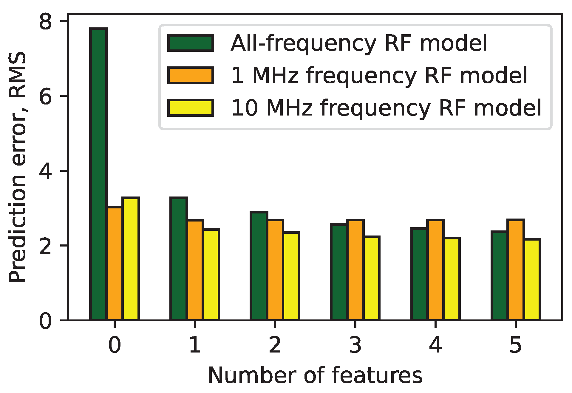
  • Random forest (RF) regression models.
For each of the model types, we train (1) one model that takes frequency as a feature, and (2) 19 models are each optimized for a specific frequency. The RF models are configured to have 1000 decision trees in each RF and use the squared error as the splitting criteria. The accuracy of the models is compared using the root-square mean error (RMSE) metric.
It is widely known that using too many features reduces the accuracy of models due to overfitting and noise. We use a greedy algorithm to select the most important features: the signal frequency, cumulative fat levels (sum of Rx and Tx fat levels), distance between attachment points, height, and weight. In future work, this could be further optimized by choosing the most important features for each frequency range; for instance, a person’s weight is a more important feature for frequencies around 1 MHz, whereas the importance of the distance between the points peaks in the 8–9 MHz range. However, we did not pursue this here in order to avoid overfitting.

4.3. Model Evaluation

We used the scikit-learn library (https://scikit-learn.org/, accessed on 4 November 2023) to fit and evaluate the models. The evaluation consists of a 10-fold cross-validation, with a random 70:30 % train:test split in each iteration. We report the average RMSE from all 10 iterations.
Figure 8 shows the results. The main takeaways are
  • The linear regression model, with frequency as the input data, has larger errors as it fails to capture the complex, nonlinear relationship between the input variables and the signal loss.
  • For the other models, the prediction error is the highest at the lower frequencies; this decreases up to 10 MHz, reaching or going below 2 dB RMSE, and then starts increasing again.
  • If the frequency is fixed, linear regression shows a similar performance to RF.
  • RF shows even better results if the frequency is passed as a feature, likely due to the larger training dataset size.
In terms of the number and importance of the features, the most important by far is the frequency (Figure 9). Figure 9 shows a large decrease in the error between 0 and 1 features for the all-frequency model; this is due to the fact that the frequency feature is added as the first one. Adding more features improves the accuracy up to a point, but the results are diminishing, and training the model on more than five features can make the error worse.
The results suggest that a large part of the signal loss variation in the dataset, unfortunately, is not explained by the features captured in the dataset. Improving this result is planned for our future work. However, since the absolute magnitude of the error is relatively small, even knowing just the target frequency should be sufficient for most use cases, such as creating design constraints for BCC communication hardware.

5. Conclusions

This paper introduces models for characterizing the human body as a signal transmission medium. Circuit models exhibit a low RMSE (below 0.7 dB). However, they require manual fitting for good accuracy. In contrast, statistical models, particularly linear regression, demonstrate RMSE errors of around 2.0 dB in the 2 to 15 MHz frequency bands. While errors increase for frequencies beyond this range, in general, the accuracy is sufficiently high enough to enable researchers and engineers to simulate and predict anticipated signal loss in BCC systems as part of their design process.
Our analysis reveals that signal frequency is the most influential feature in predicting signal loss, and factors such as the distance between communication points and human body parameters hold secondary importance. A substantial portion of the variance in signal loss remains unexplained, suggesting a potentially fertile area for future research.

Supplementary Materials

The following supporting information can be downloaded at: https://www.mdpi.com/article/10.3390/electronics12214550/s1.

Author Contributions

Conceptualization, V.A. and A.E.; methodology, V.A. and A.E.; software, V.A. and A.E.; validation, V.A. and A.E.; investigation, V.A. and A.E.; resources, V.A. and A.E.; data curation, A.E.; writing—original draft preparation, V.A. and A.E.; writing—review and editing, V.A. and A.E.; visualization, V.A. and A.E.; supervision, A.E.; project administration, A.E.; funding acquisition, A.E. ChatGPT was used to edit the text for style and clarity. All authors have read and agreed to the published version of the manuscript.

Funding

This work was supported by the Latvian Council of Science project: “Body-Coupled Communication for Body Area Networks”, No: lzp-2020/1-0358.

Institutional Review Board Statement

The study was conducted in accordance with the Declaration of Helsinki, and approved by the Ethics Committee of the Institute of Electronics and Computer Science (protocol number Nr. 2-22, 27 June 2022).

Informed Consent Statement

Informed consent was obtained from all subjects involved in the study.

Data Availability Statement

Not available.

Conflicts of Interest

The authors declare no conflict of interest. The funders had no role in the design of the study; in the collection, analyses, or interpretation of data; in the writing of the manuscript; or in the decision to publish the results.

References

  1. Maity, S.; Das, D.; Sen, S. Wearable health monitoring using capacitive voltage-mode human body communication. In Proceedings of the 2017 39th Annual International Conference of the IEEE Engineering in Medicine and Biology Society (EMBC), Jeju Island, Republic of Korea, 11–15 July 2017; pp. 1–4. [Google Scholar]
  2. Ormanis, J.; Medvedevs, V.; Aristovs, V.; Abolins, V.; Sevcenko, A.; Elsts, A. Dataset on the Human Body as a Signal Propagation Medium. 2023. Available online: https://zenodo.org/records/8214497 (accessed on 4 November 2023). [CrossRef]
  3. Ormanis, J.; Medvedevs, V.; Sevcenko, A.; Aristov, V.; Abolins, V.; Elsts, A. Dataset on the Human Body as a Signal Propagation Medium for Body Coupled Communication. Submitt. Data Brief 2023. [Google Scholar]
  4. Medvedevs, V.; Elsts, A. Simulating the Physical Layer of Body-Coupled Communication Protocols. In Proceedings of the International Workshop on Embedded Digital Intelligence (IWoEDI’2023), Riga, Latvia, 20–22 June 2023. [Google Scholar]
  5. Aristovs, V.; Elsts, A. Model of the Human Body as Signal Transmission Medium for Body-Coupled Communication. In Proceedings of the International Workshop on Embedded Digital Intelligence (IWoEDI’2023), Riga, Latvia, 20–22 June 2023. [Google Scholar]
  6. Wegmueller, M.S.; Oberle, M.; Felber, N.; Kuster, N.; Fichtner, W. Signal transmission by galvanic coupling through the human body. IEEE Trans. Instrum. Meas. 2009, 59, 963–969. [Google Scholar] [CrossRef]
  7. Zhao, J.F.; Chen, X.M.; Liang, B.D.; Chen, Q.X. A review on human body communication: Signal propagation model, communication performance, and experimental issues. Wirel. Commun. Mob. Comput. 2017, 2017, 5842310. [Google Scholar] [CrossRef]
  8. Sen, S.; Maity, S.; Das, D. The body is the network: To safeguard sensitive data, turn flesh and tissue into a secure wireless channel. IEEE Spectr. 2020, 57, 44–49. [Google Scholar] [CrossRef]
  9. Movassaghi, S.; Abolhasan, M.; Lipman, J.; Smith, D.; Jamalipour, A. Wireless body area networks: A survey. IEEE Commun. Surv. Tutorials 2014, 16, 1658–1686. [Google Scholar] [CrossRef]
  10. Tang, T.; Yan, L.; Park, J.H.; Wu, H.; Zhang, L.; Li, J.; Dong, Y.; Lee, B.H.Y.; Yoo, J. An active concentric electrode for concurrent EEG recording and body-coupled communication (BCC) data transmission. IEEE Trans. Biomed. Circuits Syst. 2020, 14, 1253–1262. [Google Scholar] [CrossRef]
  11. Maity, S.; Chatterjee, B.; Chang, G.; Sen, S. BodyWire: A 6.3-pJ/b 30-Mb/s- 30-dB SIR-tolerant broadband interference-robust human body communication transceiver using time domain interference rejection. IEEE J. Solid-State Circuits 2019, 54, 2892–2906. [Google Scholar] [CrossRef]
  12. Lucev, Ž.; Krois, I.; Cifrek, M. A capacitive intrabody communication channel from 100 kHz to 100 MHz. IEEE Trans. Instrum. Meas. 2012, 61, 3280–3289. [Google Scholar] [CrossRef]
  13. Song, Y.; Hao, Q.; Zhang, K. Review of the modeling, simulation and implement of intra-body communication. Def. Technol. 2013, 9, 10–17. [Google Scholar] [CrossRef]
  14. Maity, S.; He, M.; Nath, M.; Das, D.; Chatterjee, B.; Sen, S. Bio-physical modeling, characterization, and optimization of electro-quasistatic human body communication. IEEE Trans. Biomed. Eng. 2018, 66, 1791–1802. [Google Scholar] [CrossRef]
  15. Modak, N.; Nath, M.; Chatterjee, B.; Maity, S.; Sen, S. Bio-physical modeling of galvanic human body communication in electro-quasistatic regime. IEEE Trans. Biomed. Eng. 2022, 69, 3717–3727. [Google Scholar] [CrossRef]
  16. Park, J.; Garudadri, H.; Mercier, P.P. Channel modeling of miniaturized battery-powered capacitive human body communication systems. IEEE Trans. Biomed. Eng. 2016, 64, 452–462. [Google Scholar]
  17. Ito, K.; Hotta, Y. Signal path loss simulation of human arm for galvanic coupling intra-body communication. J. Adv. Simul. Sci. Eng. 2016, 3, 29–46. [Google Scholar] [CrossRef]
  18. Wen, E.; Sievenpiper, D.F.; Mercier, P.P. Channel characterization of magnetic human body communication. IEEE Trans. Biomed. Eng. 2021, 69, 569–579. [Google Scholar] [CrossRef] [PubMed]
  19. Asan, N.B.; Hassan, E.; Perez, M.D.; Shah, S.R.M.; Velander, J.; Blokhuis, T.J.; Voigt, T.; Augustine, R. Assessment of blood vessel effect on fat-intrabody communication using numerical and ex-vivo models at 2.45 GHz. IEEE Access 2019, 7, 89886–89900. [Google Scholar] [CrossRef]
  20. Demir, A.F.; Ankarali, Z.; Liu, Y.; Abbasi, Q.H.; Qaraqe, K.; Serpedin, E.; Arslan, H.; Gitlin, R.D. In vivo wireless channel modeling. arXiv 2019, arXiv:1902.08199. [Google Scholar]
  21. Jiang, W.; Bos, T.; Dehaene, W.; Verhelst, M.; D’hooge, J. Modelling of channels for intra-corporal ultrasound communication. In Proceedings of the 2018 IEEE International Ultrasonics Symposium (IUS), Kobe, Japan, 22–25 October 2018; pp. 1–4. [Google Scholar]
  22. Callejón, M.A.; Reina-Tosina, J.; Naranjo-Hernandez, D.; Roa, L.M. Measurement issues in galvanic intrabody communication: Influence of experimental setup. IEEE Trans. Biomed. Eng. 2015, 62, 2724–2732. [Google Scholar] [CrossRef]
  23. Maity, S.; Mojabe, K.; Sen, S. Characterization of human body forward path loss and variability effects in voltage-mode hbc. IEEE Microw. Wirel. Components Lett. 2018, 28, 266–268. [Google Scholar] [CrossRef]
  24. Störchle, P.; Müller, W.; Sengeis, M.; Lackner, S.; Holasek, S.; Fürhapter-Rieger, A. Measurement of mean subcutaneous fat thickness: Eight standardised ultrasound sites compared to 216 randomly selected sites. Sci. Rep. 2018, 8, 16268. [Google Scholar] [CrossRef]
  25. Metshein, M. Wearable Solutions for Monitoring Cardiorespiratory Activity. Ph.D. Thesis, Tallinn University of Technology, Tallinn, Estonia, 2018. [Google Scholar]
Figure 1. Electrical circuit model #1, based on Song’s et al. work [13].
Electronics 12 04550 g001
Figure 2. Current paths on the right side of model #1.
Electronics 12 04550 g002
Figure 3. The internal structure of the impedances, Z i .
Electronics 12 04550 g003
Figure 4. Electrical circuit model #2 of the human body.
Electronics 12 04550 g004
Figure 5. Amplitude-frequency response of the body in a particular measurement. Subject ID: 2695, loin to knee transmission.
Electronics 12 04550 g005
Figure 6. Additional amplitude-frequency response results for two more loin-to-knee measurements.
Electronics 12 04550 g006
Figure 7. Signal loss correlation with example features at different frequencies.
Electronics 12 04550 g007
Figure 8. Accuracy comparison for the predictive models.
Electronics 12 04550 g008
Figure 9. Accuracy, depending on the number of features for RF models. “0 features” on the x-axis corresponds to a model that returns the mean signal loss value for each frequency.
Electronics 12 04550 g009
Table 1. Input variables used as model features.
NameUnits
Signal variables
FrequencyHz
Measurement point variables
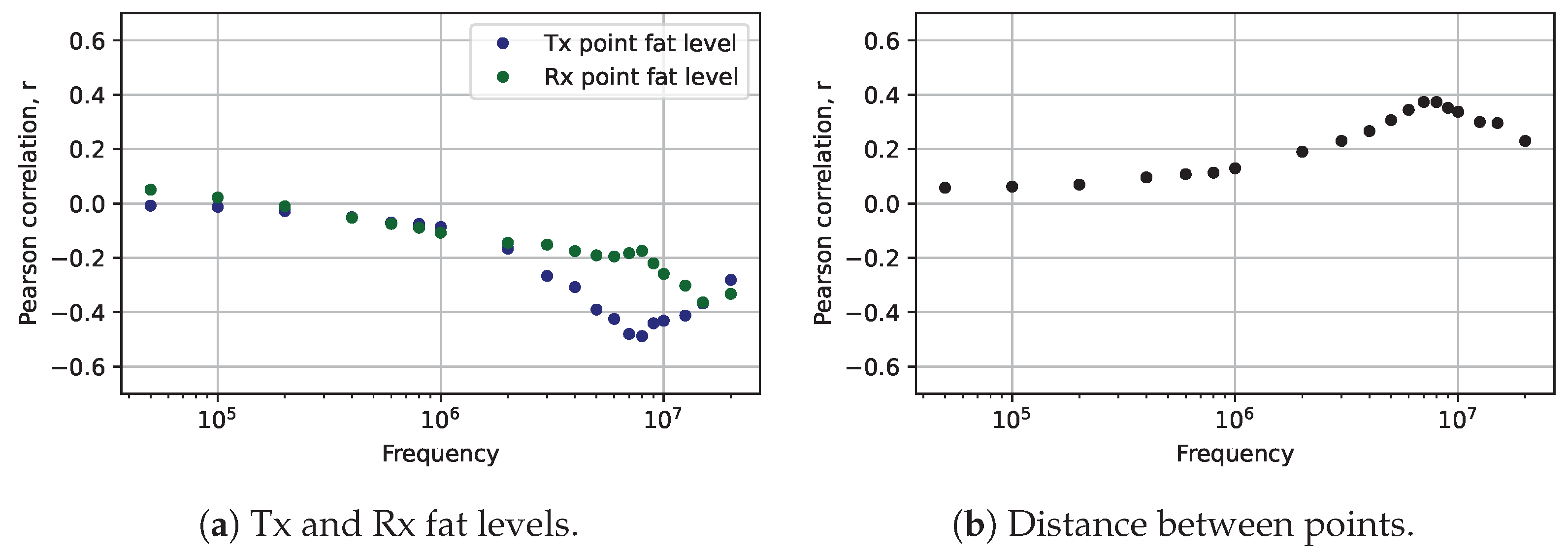
Distance between pointsrelative units
Tx point fat levelrelative units
Rx point fat levelrelative units
Human body variables
Heightcm
Weightkg
BMIkg/m 2
Body fat%
MaleBoolean
Age groupyears
Disclaimer/Publisher’s Note: The statements, opinions and data contained in all publications are solely those of the individual author(s) and contributor(s) and not of MDPI and/or the editor(s). MDPI and/or the editor(s) disclaim responsibility for any injury to people or property resulting from any ideas, methods, instructions or products referred to in the content.

