1. Introduction
Conflict analysis [
1,
2,
3] aims to analyze complex conflict situations with appropriate models by studying the conflict relationships between individuals or groups on issues, identifying the internal causes of conflict and providing some guidance for conflict resolution in intelligent decision making such as labor negotiation [
4], diplomatic relations [
5], and urban planning [
6].
Many scholars have proposed various models for conflict analysis from different perspectives. Pawlak [
5] first considered the uncertainty of agents’ attitudes toward issues and divided the agents into three groups (i.e., coalition, neutrality, and conflict). Yao [
7] extended the Pawlak model [
5] by examining three levels of conflict and proposed three-way conflict analysis. Lang et al. [
8] further improved the Yao model [
7] by employing an alliance measure and a conflict measure. In addition, considering uncertainty and data complexity in actual conflict situations, Lang et al. [
9] used Pythagorean fuzzy sets to describe conflict situations and proposed a Bayesian minimal risk theory based conflict analysis method. Li et al. [
10] proposed a conflict analysis model to cope with trapezoidal fuzzy numbers in agents’ attitudes toward issues. Yang et al. [
11] investigated a three-way conflict analysis to deal with diverse rating types in situation tables. Suo et al. [
12] studied a three-way conflict analysis model to deal with incomplete three-valued situation tables. Furthermore, since psychological factors and risk attitudes of agents may affect the results of conflict analysis, Wang et al. [
13] proposed a compound risk preference model for three-way decision based on different types of risk preferences.
Zhi et al. [
14] introduced a three-way concept for conflict analysis [
15]. Three-way concept analysis was proposed in [
15] by combining three-way decision theory [
16,
17,
18,
19,
20] and formal concept analysis [
21,
22], with the ability of describing the properties that objects possess in common and those that they do not possess in common [
23,
24]. Zhi et al. [
14] analyzed the conflict relationships between agents and identified the binary relationships between sets of agents and sets of issues by using three-way concepts, and then analyzed the causes of conflict. The above studies were conducted in the case that agents are completely trustworthy. In some situations (for example, in network); however, agents may be untrustworthy. To this end, Zhi et al. [
25] proposed a multilevel conflict analysis that analyzed and resolved uncertainty in agents’ trustworthiness and uncertainty in agents’ attitudes toward issues. However, in [
25], when describing the consistency of agents using fuzzy concepts, only the common agreement consistency is considered and the common opposition consistency is ignored. This may lead to a misjudgment of conflict in some cases. For example, when agents oppose an issue, according to [
25] the agents are inconsistent on this issue, but in fact, agents are consistent.
On the other hand, when agents have disputes, it is necessary to find appropriate conflict resolution strategies to promote cooperation among them. To this end, Sun et al. [
26] constructed a probabilistic rough set model and provided an effective method to find the feasible consensus strategy to facilitate the resolution of conflict situations. To select an effective feasible strategy, Xu et al. [
4] formulated the criteria for selecting feasible strategies based on consistency measurement of cliques. Based on game-theoretic rough sets, Bashir et al. [
1] designed a novel conflict resolution model by constructing a game among all agents, computing the payoff of different strategies, and classifying them according to the equilibrium rules. From the perspective of multi-criteria decision analysis, Du et al. [
2] introduced three kinds of relations among agents into multi-criteria large-scale group decision making in linguistic context, obtained the coalition of decision models and the weights of criteria and finally proposed a conflict coordination and feedback mechanism to solve conflicts.
Most of the existing solution strategies resolve conflicts by selecting an optimal subset of issues most agents agree on. However, if conflicts have not yet reached a serious level, some compromises can be made through third-party mediation to promote cooperation between the agents. For example, Iran and Saudi Arabia have resumed diplomatic relations after China-mediated talks. Therefore, this paper considers changing the attitudes of agents to make them reach a consensus. Since such changes will bring a certain cost, it is necessary to measure the costs to determine an optimal change. In addition, the cost may also change as trust degree is introduced and changed. Consequently, conflict resolution strategies that only consider costs, without considering trust, are often ineffective.
In order to solve the above problems, this paper introduces an
L-fuzzy three-way concept lattice (
L-3WCL) [
27], which is mainly used in knowledge representation [
28] and fuzzy three-way concept lattices reduction [
29], to conflict analysis and resolves the conflict using the dynamic programming method of the knapsack problem [
30,
31,
32]. As a result, a hybrid conflict analysis model is developed. The model first employs
L-fuzzy three-way concept to capture the issues on which agents commonly agree and the issues which they commonly oppose, and then measures the relative inconsistency of a set of agents. By relative inconsistency, we identify the state of a set of agents and categorize the issues into different types, which may help us find the causes of conflict. To facilitate cooperation between agents, we act as a third-party mediator, seeking to compromise between the agents at minimal cost to reach a consensus. We model this problem as a knapsack problem, which is a combinatorial optimization problem that can be solved using dynamic programming method. Finally, we propose an optimal attitude change strategy based on dynamic programming and solve conflicts with minimum cost. Furthermore, we verify the effectiveness of this strategy in intelligent decision-making instances such as business decision making.
Section 2 will briefly review the models in [
5,
25].
Section 3 analyzes the shortcomings of the fuzzy-concept-lattice-based conflict analysis model and proposes an
L-3WCL-based conflict analysis model.
Section 4 develops an optimal attitude change strategy and illustrates the effectiveness of the strategy with a case study. Finally,
Section 5 concludes the paper with an outlook.
3. -3WCL Based Conflict Analysis Model
The Zhi model can effectively analyze conflict situations with the uncertainty of agents in trustworthiness, but it may lead to misjudgment of conflicts. Example 1 illustrates the cause of misjudgment.
Example 1. Let be a CAIS, where , and .
For K, since the attitudes of agents and towards issue y are both negative, they reach a consensus on y; therefore, the inconsistency should be 0. However, according to the Zhi model, when using the Łukasiewicz implication, for , according to Definitions 8 and 9, and . Thus, the inconsistency of agents and on y is 1, indicating that the attitudes of the two agents are inconsistent. Similar problems also exist in the Zhi model when using other commonly used implication operators.
From Example 1, we can see that the Zhi model misjudges the conflict. This is due to the fact that the Zhi model only considers the common agreement of agents as consistency and the common opposition of agents as inconsistency. Since
L-3WCL [
27] is able to characterize both the attributes that objects commonly possess and the attributes that they commonly do not possess, we will utilize
L-3WCL to describe the issues that agents commonly agree on and commonly oppose, and propose a hybrid conflict analysis method based on
L-3WCL.
Definition 10 ([
27])
. For a fuzzy formal context , define and as:where , , , , and When , and , is called an object-derived L-fuzzy three-way concept and X and are called the extent and intent of ,, respectively. All the fuzzy concepts of K form a complete lattice , called the L-3WCL of K, defined as A CAIS can be regarded as a fuzzy formal context, where represents the attitude of the agent x towards the issue y, and represents the trust degree of x. By Definition 10, represents the consistency degree of X in agreeing with the issue y; represents the consistency degree of X in opposing y. Since the larger the value of the higher the degree of agreement, when remains constant, increases with the increase of ; in other words, is the agreement consistency. Similarly, since the larger the value of the higher the degree of opposition, when remains constant, increases with the increase of , and therefore is the opposition consistency.
Similarly, in Definition 10,
denotes the agreement consistency with the issue
y and
denotes the opposition consistency with
y. If
and
, i.e.,
is the agreement consistency of
X with
y and
is the opposition consistency of
X with
y,
returns a new set
such that
for any
(see [
27]), implying that one can increase the trust degree of
x while keeping the same agreement consistency and opposition consistency because
(see [
27])
.In our case, we require L to be {0, 0.5, 1}. In particular, we have the following conclusions.
Both and are also in {0, 0.5, 1}. If , then the set X of agents completely reach a consensus in agreeing with the issue y; if , then X partially reach a consensus in agreeing with y; and if , then X does not reach a consensus in agreeing with y. Similar analysis applies to .
The value of also falls in . In this case, if , then the agent x is fully trusted. If , then x is partially trusted; if , then x is not trusted.
Example 2. Since the Gödel implication operator is not suitable for building fuzzy logic systems [38], we will choose the Łukasiewicz implication operator for illustration. In this case, for and , we have When all the agents are trustworthy, i.e., , we have and . This is reasonable because when all the agents are trustworthy, the consistency of X will completely depend on their attitudes.
If there is an agent with , then we have , i.e., the values of and are not affected by . This is also reasonable because if the agent x is not trustworthy, their attitude can be ignored.
Based on the agreement consistency and opposition consistency, the comprehensive consistency can be defined.
Definition 11. Let be a CAIS and . The comprehensive consistency of X on the issue is defined as According to Definition 11, we can see that
If and , then the set X of agents reaches a complete consensus both on agreeing with y and on opposing y. In fact, when using the Łukasiewicz implication operator, for and , if for all the agents , then we have and , i.e., when the attitudes of all the agents are ignorable, one can conclude and . Similarly, if for all the agents , implies , then we have and , i.e., when the trustworthiness and the attitudes of agents are uncertain, one can also conclude and . In both the cases, it can be considered either that X is unanimously agreeing on y or that X is unanimously opposing on y, and y is an alliance issue for X.
If and , then X reaches a complete consensus on agreeing with y and does not reach a complete consensus on opposing y. In this case, the agents within X have achieved a unanimous agreement on y. Similarly, if and , then X reaches a complete consensus on opposing y but does not reach a complete consensus on agreeing with y. It can be considered that the agents in X have achieved a unanimous opposition on y. In both the cases, X achieves a consensus, i.e., , and y is an alliance issue for X.
If and , then there must exist at least one pair of agents with opposite attitudes. Therefore, its comprehensive consistency is 0. In fact, when using the Łukasiewicz implication operator, if , then there must exist such that , which implies . Similarly, if , then there must exist such that , which implies , yielding . Hence, the attitudes of agents and towards y are opposite, indicating that X does not reach a consensus, i.e., . At this point, y is a conflict issue of X.
If and , then X reaches a partial consensus on agreeing with y but does not reach a consensus on opposing y. In this case, X only partially agrees on y. Similarly, if and , then the agents reach a partial consensus on opposing y but does not reach a consensus on agreeing with y. Thus, X only partially agrees on y. If and , X partially reaches a consensus on agreeing with and opposing y. This indicates that X reaches a partial consensus on y. In all the three cases, X only reaches a partial consensus on y, i.e., , and y is a neutral issue of X.
In Example 1, because the Zhi model does not consider the opposition consistency, a discrepancy with the actual situation occurs when analyzing the consistency of agents. Definition 11 considers both the agreement and opposition consistency, leading to a more reasonable result than the Zhi model. For example, for the issue y in Example 1, two agents and have the agreement consistency , the opposition consistency , and the comprehensive consistency , which is in line with the actual situation.
The relative inconsistency of a set of agents can be determined by the comprehensive consistency over all the issues.
Definition 12. Let be a CAIS and . Define the relative inconsistency of X as Let and be two thresholds such that . For , if , then X is called an alliance set of agents; if , then X is called a neutral set of agents; if , then X is called a conflict set of agents.
The difference between the relative inconsistency (Equation (
17)) and the inconsistency in the Zhi model (Equation (
8)) is illustrated by Example 3.
Example 3. Table 1 shows a CAIS , where and . If , then according to the Zhi model, we have , , , , , and . By Equation (8) we can obtain . According to the proposed model, we have , , , , , and , yielding . From the calculation process, it can be seen that the two models are consistent on the set , but on the set , the Zhi model considers that the set is completely inconsistent on and (i.e., and ), while the proposed model considers that the set is completely consistent on (i.e., ) and partially consistent on (i.e., ). Intuitively, the attitude of X on is consistent and therefore the calculation result of the proposed model is reasonable; for , if the consistency of the attitudes of X towards this issue is considered to be 0, the same result can be obtained in the case of and . In other words, the result of the Zhi model on cannot distinguish the two cases: 1. and ; 2. and . When considering the subset , by Equation (8), we can obtain and by Equation (17), we can obtain . Thus, when the issue is not taken into consideration, will decrease from to , while will decrease from to . Obviously, the decrease of is greater than that of . This is because the Zhi model considers that X has conflicts not only on issue , but also on issues and , and thus removing issue does not eliminate the conflicts in X. The proposed model considers that X has the highest level of conflict on and thus removing results in a greater decrease in the inconsistency of X. From Example 3, we can derive
, a general relationship between Equations (
8) and (
17).
Theorem 1. Let be a CAIS and . Then, we have .
Proof of Theorem 1. For any , we have and thus the conclusion holds by Definitions 11 and 12. □
Theorem 1 is obvious, because the proposed model captures both the agreement consistency and the opposition consistency of agents towards issues, while the Zhi model only captures the agreement consistency of agents towards issues. Thus, compared to the Zhi model, the proposed model reduces the inconsistencies of the sets of agents.
Theorem 2. Let be a CAIS, and X, . If , then we have
Proof of Theorem 2. If , for any , then we have , and by the definition of and , when is constant, if increases, then both and will decrease. Thus, we obtain and . By Definitions 11 and 12, the conclusion holds. □
Theorem 2 shows that the more agents there are, the higher the probability of inconsistency. In fact, suppose that
X,
satisfy
,
,
, …,
. One can easily obtain
for any
y and thus
. In other words, when the trust degree of agent
increases from
to
, since
, the importance of this agent’s opinion in
X increases, leading to a decrease in the agreement consistency
or the opposition consistency
, which in turn leads to an increase in the inconsistency of
X. Similarly, suppose that
satisfies
,
, …,
. One can easily obtain
for any
y and thus
, i.e., the increase of the trust degree in agent
leads to the increase of the inconsistency in
X. Continue the process and suppose that
satisfies
,
,
, …,
. Then, one can easily obtain
and thus
. In summary, we have
By Definition 12, one can determine the state of a set of agents. If the set is allied, one may be more concerned about whether the set is unanimously agreed on or opposed some issues; if it is neutral, then the set is partially agreed and one may be more concerned about the issues that the agents are partially agreed on and the issues that they oppose; if it is conflicted, then the set does not reach a consensus on some issues and one may have to analyze the reasons of the conflicts. For this purpose, one should further analyze issues according to their states.
Definition 13. Let be a CAIS. For and ,
- 1
If and , then y is called a unanimous agreement issue of X. The unanimous agreement set of issues of X is defined as - 2
If and , then y is called a unanimous opposition issue of X. The unanimous opposition set of issues of X is defined as - 3
If and , then y is called a unanimous issue of X. The unanimous set of issues of X is defined as - 4
If and , then y is called an agreement-neutral issue of X. The agreement-neutral set of issues of X is defined as - 5
If and , then y is called an opposition-neutral issue of X. The opposition-neutral set of issues of X is defined as - 6
If and , then y is called a completely neutral issue of X. The completely neutral set of issues of X is defined as - 7
If and , then y is called a conflict issue of X. The conflict set of issues of X is defined as
By Definition 13, the attitude of a set of agents on an issue can be derived. For and , if , then X agrees unanimously on y; if , then X opposes unanimously y; if , as mentioned before, then either X agrees unanimously on y or X opposes unanimously y. Since X is unanimous on y when , these issues are collectively referred to as alliance issues. If , then X is neutral on agreeing on y; if , then X is neutral on opposing y; if , then X is neutral on either agreeing on or opposing y. Since X is neutral on y when , these issues are collectively referred to as neutral issues. If , then X is in conflict on y, and these issues will be called conflict issues. Neutral and conflict issues are collectively referred to as non-coalition issues.
Theorem 3. Let be a CAIS, and X, . If , then
- 1
- 2
- 3
- 4
- 5
- 6
- 7
- 8
.
Proof of Theorem 3. (1) If , then we have and . Since , we obtain and , i.e., and , and hence .
(2) If , then we have and . Since , we obtain and , i.e., and , and hence .
(3) If , then we have and . Since , we obtain and , i.e., and . If and , then we have ; if and , then we have .
The proofs of (4), (5), (6), (7), and (8) are similar. □
Theorem 3 (1) states that the more agents there are, the fewer issues they reach a consensus on. Theorem 3 (2) states that the more agents there are, the more conflict issues there are. Theorem 3 (3) and Theorem 3 (4) state that the unanimous agreement issues or unanimous opposition issues may become the unanimous issues when there are fewer agents. Theorem 3 (5) and Theorem 3 (6) state that the agreement-neutral issues or the opposition-neutral issues may become conflict issues when there are more agents. Theorem 3 (7) states that the completely neutral issues may become the agreement-neutral issues or the opposition-neutral issues or the conflict issues when there are more agents. Theorem 3 (8) states that the completely neutral issues may become the unanimous agreement issues or the unanimous opposition issues or the unanimous issues when there are fewer agents.
Example 4. Table 2 shows a CAIS , where and . For and , according to Definition 10, we can obtain , , , , , and ; therefore, , . Similarly, we have , , , , , and ; therefore, , and . When the number of agents increases, i.e., X becomes , according to Theorem 3 (1), the unanimous issues become fewer, from to . When the number of agents decreases, i.e., becomes X, according to Theorem 3 (3), the unanimous agreement issue become the unanimous issue; according to Theorem 3 (8), the completely neutral issues become the unanimous agreement issues. In addition, it can be found that although , has no inclusion relation with .
According to the above discussion, for a given set X of agents, the state of X and its attitude towards each issue can be determined. When the trust degrees of agents changes frequently; however, the workload of performing conflict analysis may be huge. It is easy to conclude that for a set of agents containing n agents, the number of sets of agents under is ; even when , the number of sets of agents will be . In fact, the basic nature of L-3WCL states that sets of agents with different trust degrees may produce the same conflict analysis results. Specially, for the sets and of agents with different trust degrees, if and , then their conflict analysis results are exactly the same. In other words, the number of conflict analysis results is equal to the number of L-fuzzy three-way concepts, much smaller than . Therefore, in order to reduce the workload, we can establish L-3WCL to calculate all possible conflict analysis results, and when trust degrees change, we only need to find the result corresponding to X. In addition, by analyzing L-3WCL, we can also observe the change of conflict analysis results when trust degree changes.
In , the extent of a concept represent a set of agents with different trust degrees, and the intent represent the agreement degree and opposition degree. For any set X of agents, the corresponding fuzzy three-way concept can be found in , and the relative inconsistency and sets of issues , , , , , , and can be derived by Definitions 12 and 13.
For three concepts , and in , if , then . According to Theorems 1 and 2, if the trust degrees of raises to , the conflict issues in must be the conflict issues in , the opposition-neutral issues must be the opposition-neutral issues or the conflict issues in , the agreement-neutral issues must be the agreement-neutral issues or the conflict issues in , the complete neutral issues must be the complete neutral issues, the opposition-neutral issues, and the agreement-neutral issues or the conflict issues in . If the trust degrees of decreases to , then the unanimous issues in must be the unanimous issues in , the unanimous agreement issues must be the unanimous agreement issues or unanimous issues in , the unanimous opposition issues must be the unanimous opposition issues or the unanimous issues in , the completely neutral issues must be the completely neutral issues, the unanimous agreement issues, the unanimous opposition issues, or the unanimous issues in .
In the following, we illustrate the L-3WCL based conflict analysis model in Example 5.
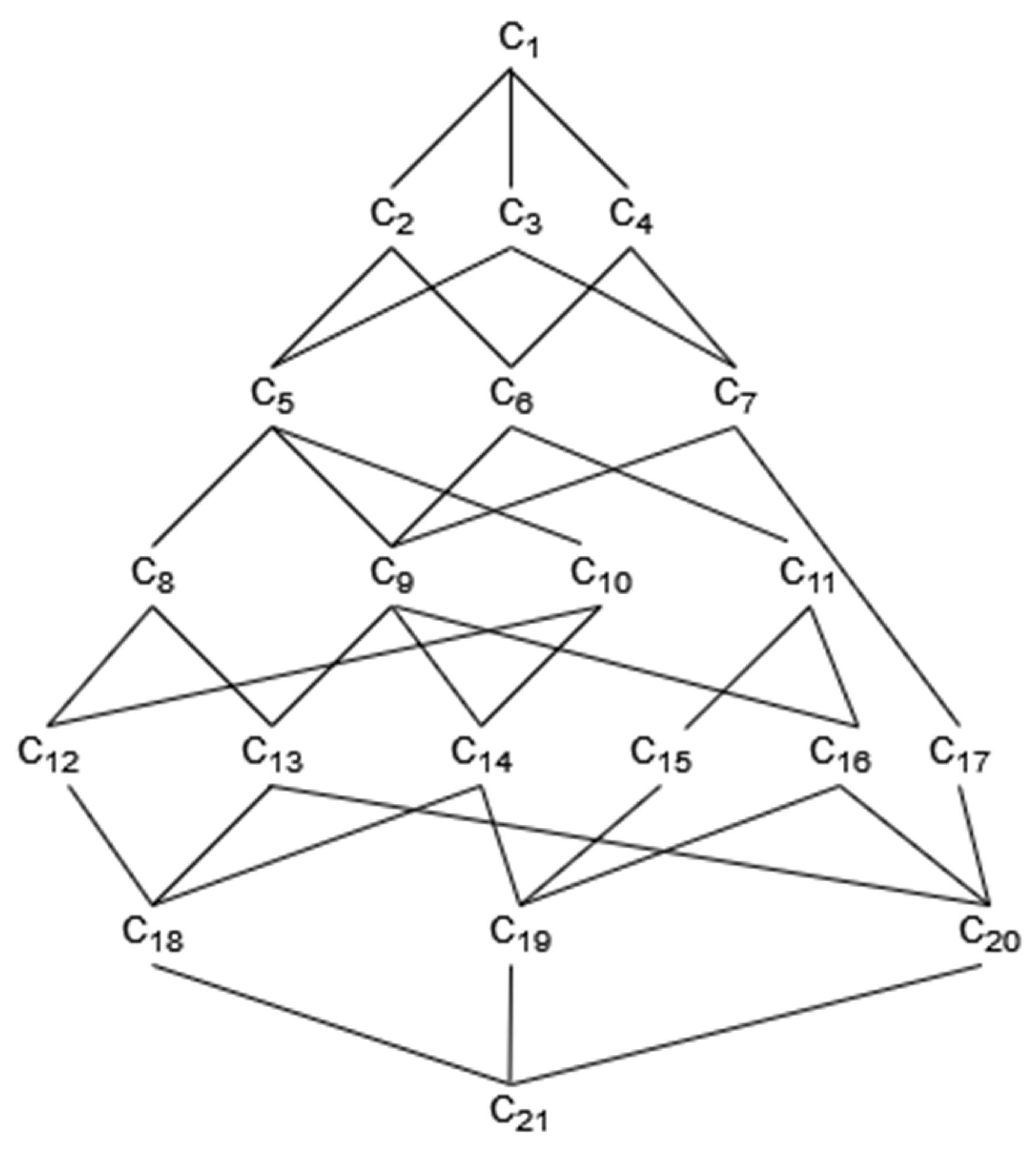
Example 5. Consider the situation in which some agents are discussing some strategies for the development of an enterprise. Since the circumstances and the interests of agents may be different, there may be some conflicts among agents. Assume that three agents and four development strategies constitute a CAIS , where and with representing talent introduction, representing project management, representing marketing and sales, and representing technology development. The attitude of each agent towards each issue is shown in Table 3. For example, agent has a positive attitude towards , agent has a negative attitude towards , and agent has a neutral attitude towards . Since agents have different discourse powers, we adopt three levels of analysis, i.e., agent has very large discourse power, agent has relatively small discourse power, and agent has no discourse power. For example, when the discourse power of agent is relatively small, the discourse power of agent is very large, and agent has no discourse power, we represent it as . When Łukasiewicz implication operator is used, of K is shown in Figure 1. The concepts in Figure 1 and the corresponding conflict analysis results are shown in Table 4. In Table 4, for the concepts with at least two agents in the extents, the conflict analysis results obtained are the consistency of different agents; for the concepts with only one agent in the extents, the conflict analysis results obtained are the consistency of the agent for different issues; for the concept having no agents in the extent, the conflict analysis results are not meaningful. The conflict analysis result of a set of agents can be used to infer the conflict analysis results of other sets of agents. For example, the conflict issue of is ; according to Theorem 3, we can infer that issue must also be a conflict issue of ; the opposition-neutral issues and of must be the opposition-neutral issues or the conflict issues of ; and the agreement-neutral issue of must be an agreement-neutral issue or a conflict issue of .
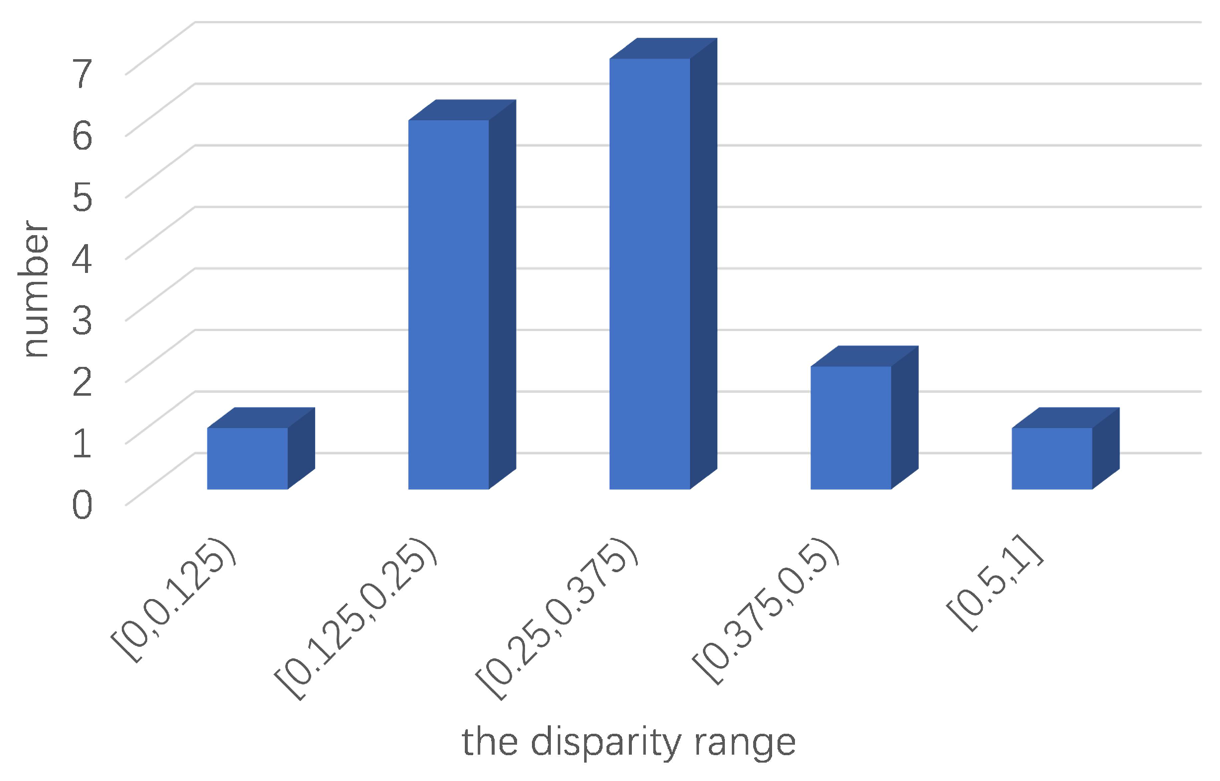
The extents of the concepts in Table 4 contain only some sets in and other sets of agents can be described by the corresponding concepts in , as shown in Table 5. Combining Table 4 and Table 5, all the conflict analysis results of all sets of agents can be calculated. For example, in Table 5, we can see that for the set of agents , i.e., has a relatively large discourse power, has a very large discourse power, and has no discourse power, the corresponding concept can be obtained as , and , , , , , , and . This indicates that the agents in X reach a complete consensus on opposing the marketing and sales issue , a partial consensus on agreeing on the project management issue and opposing the technology development issue , and a partial consensus on the talent introduction issue . Since , the conflict between agents is small. When applying the Zhi model to Table 3, the conflict analysis results can be obtained, as shown in Table 6. The comparison with the proposed model is also shown in Table 6. According to Table 6, among the 17 results obtained by the Zhi model, 16 results are different from those obtained by the proposed model, indicating that there is a 94% probability that the Zhi model is problematic. The proposed model reduces the inconsistency in 16 results compared with the Zhi model, as shown in Figure 2. According to Figure 2 and Table 6, it is clear that the inconsistency decreases as the number of agents decreases, which verifies the correctness of Theorem 2. It can be observed that the difference between the two models occurs when the opposition consistency of X for an issue y is greater than the agreement consistency . This is because the consistency in the Zhi model is the agreement consistency, and the consistency in the proposed model is the maximum of the opposition consistency and the agreement consistency. By examining the disparity distribution of two inconsistencies which is shown in Figure 3, we can observe that the disparities between the two inconsistencies are primarily situated in the interval . These variations in value are relatively minor. On the interval , there are two results with a large disparity between the two inconsistencies, which is mainly caused by the Zhi method misclassifying an alliance issue as a conflict issue. In particular, the disparity between the two inconsistencies in the 14th result is 0.5, the largest disparity among all the results. This is because the Zhi model treats the two issues and , which are unanimously opposed by X, as conflict issues, and the proposed model considers the two issues as the unanimous opposition issues. This means that if the Zhi model determines that X is a non-coalition, the proposed model must consider that X is an alliance. Thus, the disparity between the two inconsistencies directly affects the disparity in the states of X. Similarly, in the 15th-16th results, the inconsistency of the Zhi model indicates that the sets of agents are divergent and neutral on several issues, and no consensus is reached. The inconsistencies of the proposed model are all 0 and the sets of agents reach a consensus on all the issues. 4. Conflict Resolution Based on the Proposed Model
In
Section 3, we examined the alliance issues, the neutrality issues, and the conflict issues of a given set of agents. For a set of agents in alliance, minimal divergence exists in the set, enabling the agents to easily reach a consensus. A non-alliance set of agents may experience substantial divergence in issues, presenting challenges for consensus-building among the agents. To address these conflicts, it becomes crucial to develop strategies that eliminate the divergence between agents and mitigate the relative inconsistency, thereby transforming the non-alliance set of agents into an alliance set.
For , it follows from Definition 12 that the relative inconsistency is determined by the comprehensive consistency of all the issues y, and thus can be decreased only by increasing . According to Definition 13, if , then we have , so the comprehensive consistency of an alliance issue cannot be increased; if , then we have , and the comprehensive consistency can be increased from 0.5 to 1, i.e., a neutral issue can be transformed into an alliance issue, thus decreasing the relative inconsistency ; if , then we have , and the comprehensive consistency can be increased from 0 to 0.5 or 1, which transforms a conflict issue into a neutral issue or an alliance issue, thus decreasing the relative inconsistency . Therefore, the relative inconsistency can be effectively decreased only by increasing the comprehensive consistency of non-alliance issues. In the following, we consider how to increase the comprehensive consistency of the issues in , , , and .
According to Definition 11, the comprehensive consistency is determined by the agreement consistency and the opposition consistency , and from Definition 10, it follows that and are jointly determined by the trust degree and the attitude . To increase , it is necessary to increase or . Depending on the nature of implication operator, and can be increased by decreasing ; however, in most conflict situations, cannot be easily changed, e.g., when an enterprise makes a development plan, the discourse powers of agents in different positions are generally fixed. Therefore, in order to increase or , it is necessary to change agents’ attitudes towards issues.
Let
be a CAIS and
. In order to increase
,
can be increased by changing the attitudes of agents. If
, then in order to increase
to 0.5, according to the definition of
, the set of agents whose attitudes should be changed is
For
, we have
; otherwise, we have
. Therefore, we denote
and then
.
If
, then in order to increase
to 1, the set of agents whose attitudes should be changed is
where
.
If , then in order to increase to 1, the set of agents whose attitudes should be changed is .
Similarly, in order to increase
, it is also feasible to increase
by changing the attitudes of the agents. If
, then in order to increase
to 0.5, according to the definition of
, the set of agents whose attitude should be changed is
For
, we have
; otherwise, we have
. Therefore, we denote
and then
.
If
, then in order to increase
to 1, the set of agents whose attitudes should be changed is
where
.
If , then in order to increase to 1, the set of agents whose attitudes should be changed is .
The following conclusions hold.
Theorem 4. Let be a CAIS, and .
- 1
Suppose .
- (a)
If , then can be increased from 0.5 to 1 at a cost of at least . In this case, the attitude of x needs to be increased to 1 for and and to 0.5 for and .
- (b)
If , then can be increased from 0.5 to 1 at a cost of at least . In this case, if , then the attitude of x needs to be reduced to 0 for and ; if , then the attitude of x needs to be reduced to 0 for and and to 0.5 for and .
- 2
Suppose .
- (a)
If , then can be increased from 0.5 to 1 at a cost of at least . In this case, the attitude of x needs to be reduced to 0 for and and to 0.5 for and .
- (b)
If , then can be increased from 0.5 to 1 at a cost of at least . In this case, the attitude of x needs to be increased to 1 for and and to 0.5 for and .
- 3
Suppose .
- (a)
If , then can be increased from 0.5 to 1 at a cost of at least . In this case, the attitude of x needs to be increased to 1 for and and to 0.5 for and .
- (b)
If , then can be increased from 0.5 to 1 at a cost of at least . In this case, the attitude of x needs to be reduced to 0 for and and to 0.5 for and .
- 4
Suppose .
- (a)
If , then can be increased from 0 to 0.5 at a cost of at least . In this case, the attitude of x needs to be increased to 0.5 for and .
- (b)
If , then can be increased from 0 to 0.5 at a cost of at least . In this case, the attitude of x needs to be reduced to 0.5 for and .
- (c)
If , then can be increased from 0 to 1 at a cost of at least . In this case, the attitude of x needs to be increased to 1 for and and to 0.5 for and .
- (d)
If , then can be increased from 0 to 1 at a cost of at least . In this case, if , then the attitude of x needs to be reduced to 0 for and ; if , then the attitude of x needs to be reduced to 0 for and and to 0.5 for and .
Proof of Theorem 4. 1. For , in order to increase from 0.5 to 1, we can increase from 0.5 to 1, or increase from 0 to 1.
In order to increase from 0.5 to 1, according to the definition of , the values of of all the agents in must be increased from 0.5 to 1. If , then consider the following three cases.
(1) If , then we have , and by Proposition 1 (2), we have . In order to increase the value of from 0.5 to 1, we need to change to . Since , we have and . Thus, the cost is .
(2) If , then we have and thus ; otherwise, by Proposition 1 (1), if , then we have . In order to increase the value of from 0.5 to 1, we need to change to . Since , we have or and thus . Therefore, the cost is .
(3) If , then by Proposition 1 (1), does not exist, such that .
Therefore, the total cost is .
In order to increase from 0 to 1, according to the definition of , the values of of all the agents in must be increased to 1. Since and , and are disjoint, we need to consider the three sets, respectively.
If , then consider the following three cases.
(1) If , then, since , we have . In order to increase of all the agents in from 0 to 1, we need to change to . Since , we have and thus . The cost is .
(2) If , then because , we have . Since , we have . At this time, we need to change to , so we have or . If , then according to Proposition 1 (3), we have and thus , which is contradictory to . Thus, we have , and the cost is .
(3) If , then does not exist, such that .
Therefore, the total cost is .
If , then consider the following three cases.
(1) If , then in order to increase from 0 to 1, we need to change to . Since , we have and thus . The cost is .
(2) If , then since , we have . Since , we have or . If , according to Proposition 1 (3), we can conclude and thus , which is contradictory to . Therefore, we have , i.e., . In this case, and the cost is .
(3) If , then does not exist, such that .
Therefore, the total cost is .
If , then consider the following three cases.
(1) If , we have , and only when , holds. In order to increase the value of from 0.5 to 1, we need to change to . Since , we have and thus . Thus, we have , and the cost is .
(2) If , then we have and thus , yielding . Since , we have or . If , then we have , which is contradictory to , and thus . In order to increase the value of from 0.5 to 1, we need to change to . Since , we have or , and thus or . At this time, we have , and the cost is .
(3) If , then does not exist, such that .
Therefore, the total cost is .
In summary, in order to increase from 0.5 to 1, we can increase to 1 at the cost of , or increase to 1 at the cost of . If , then can be increased to 1 at a cost of at least . Otherwise, can be increased to 1 at a cost of at least .
Thus, if is increased to 1, then we need to increase the attitude of x with and to 1, as well as increasing the attitude of x with and to 0.5. If is increased to 1, and if , then we need to reduce the attitude of x with and to 0. If , then the attitude of x with and should be reduced to 0, and the attitude of x with and should be reduced to 0.5.
Other results can be proved similarly. □
By Definition 13, if , then X is a neutral or conflict set of agents. In order to transform X into an alliance set, it is necessary to reduce to , with the difference of .
In order to reduce , it is necessary to increase . If , then can be increased either to 0.5 or to 1; if , then can be increased to 1.
Now, denote the number of issues such that
as
and the number of issues such that
as
. According to Definition 12, we have
Denote by
the number of issues whose
need to be increased from 0 to 0.5; denote by
the number of issues whose
need to be increased from 0 to 1; denote by
the number of issues whose
need to be increased from 0.5 to 1. Thus, the relative inconsistency will become
and the difference is
We require
, i.e.,
,
and
satisfy Equation (
37)
Obviously, there may be different values of
,
and
that satisfy Equation (
37) and can transform
X into an alliance set. Since the cost of increasing
varies for different issues
y, in real life, people tend to seek the least costly way to make decisions. Therefore, it is necessary to consider which issues to change so that the cost of transforming
X into an alliance set is minimal.
For an issue y, there may be more than one way to increase . For , can only be increased from 0.5 to 1 with a cost of 0.5; for , can be increased from 0 to 0.5 or from 0 to 1 with a cost of 0.5 or 1. Therefore, there are at most two methods to increase for issue y, but at most one method can be chosen.
The problem can be formulated as follows. For a set of
s issues,
denotes the number of increasing methods for the
i-th issue; the variation of the
k-th increasing method for the
i-th issue is
, and the corresponding cost is
. The objective is to choose an optimal solution
, such that the sum of the costs
is minimized while the sum of variations
is not less than
, where
indicates whether the optimal solution chooses the
k-th increasing method for the
i-th issue, i.e.,
It can be observed that the problem is actually a grouped knapsack problem, which is a special kind of knapsack problem. There are several solutions to solve the knapsack problem, such as branch-and-bound method [
39], dynamic programming method [
40], and approximation algorithm [
41]. Since the dynamic programming method can solve the optimal solution quickly for smaller knapsack problems, we adopt the dynamic programming method to select the least costly set of issues. The method of solving the optimal attitude change strategy based on the dynamic programming method is shown in Algorithm 1.
| Algorithm 1 The optimal attitude change strategy based on dynamic programming method. |
Require: A CAIS , threshold , a set of agents
Ensure: An optimal attitude change strategy
- 1:
Compute , , , and according to Definition 13 - 2:
for each
y
in
do - 3:
Compute and - 4:
▹ denotes the number of increasing methods of y - 5:
▹ denotes the variation of the first increasing method of y - 6:
, ▹ denotes the cost of the first increasing method of y - 7:
end for - 8:
for each
y
in
do - 9:
Compute and - 10:
- 11:
- 12:
, - 13:
end for - 14:
for each
y
in
do - 15:
Compute and - 16:
- 17:
- 18:
, - 19:
end for - 20:
for each
y
in
do - 21:
Compute , , and - 22:
▹ the number of increasing methods is 2 - 23:
- 24:
, - 25:
▹ denotes the variation of the second increasing method of y - 26:
, ▹ denotes the cost of the second increasing method of y - 27:
end for - 28:
Compute according to Definition 12 - 29:
▹ is the amount of variations needed to transform X into an alliance set - 30:
Utilize the dynamic programming method in [ 30] or [ 31, 32] to solve the knapsack problem and obtain the optimal solution - 31:
According to M, determine the agents that need to change their attitudes, and add the agents and the issues to the corresponding sets - 32:
return , , , , ,
|
Steps 2–27 of Algorithm 1 first determine the number of increasing methods , the variation , and the cost of the k-th increasing method for issue y according to Theorem 4. Then, Algorithm 1 solves the optimal attitude change strategy by dynamic programming method in Step 30 and obtains an optimal solution . Finally, in Step 31, according to the optimal solution M and Theorem 4, Algorithm 1 identifies the agents that are required to change their attitudes towards some specific issues, and adds the pairs of agent and issue to the corresponding sets: , , , , , and .
Example 6 verifies the validity of Algorithm 1.
Example 6. For the CAIS in Example 5, given the threshold , we have . According to Table 3, we have , , , and . Since , X should be transformed into an alliance set. According to Algorithm 1, of issue can be increased from 0.5 to 1 with the variation and the cost ; of issue can be increased from 0.5 to 1 with the variation and the cost ; of issue can be increased from 0.5 to 1 with the variation and the cost ; of issue can be increased from 0 to 0.5 with the variation and the cost , or increased from 0 to 1 with the variation and the cost . According to the dynamic programming method, only and can be obtained in M. Since , we can compute . Furthermore, since and , we have . Since , we can compute . Since and , we have .
Therefore, the optimal attitude change strategy is , , i.e., changing the attitude of towards from opposing to agreeing and changing the attitude of towards from agreeing to neutral. After changing attitudes, we have , , , and , i.e., X becomes an alliance set with the minimal cost 2. The changes in conflict analysis results caused by attitude changes is shown as Figure 4. 


