Abstract
Robust control systems are a necessity for autonomous underwater vehicle (AUV) systems due to the challenges they face during operation. Many AUV control-design methods have been developed for different actuator configurations, with robustness against model parameter uncertainties, environmental disturbances, and system faults. Actuator faults can reduce the physical capabilities of a system, which can be compensated for through control re-allocation. However, the increased control allocation to the remaining actuators may cause actuator saturation and reduce controller performance. In this work, we present a depth-pitch model-based nonlinear control law that directly considers actuator saturation, and a fault-tolerant control allocation method for a hybrid AUV actuator configuration. Two types of actuator faults are considered for an underwater vehicle with a hybrid actuator configuration. The proposed controller is implemented in a simulated system, and its trajectory tracking performance is compared with a baseline system without fault or saturation tolerance. To determine the utility of the proposed saturation and fault tolerance control methods, the tracking performance in these simulations is quantified in terms of the settling time, post-fault peak values, and root mean square of the depth and pitch errors.
1. Introduction
Autonomous underwater vehicles (AUVs) perform a variety of operations such as environmental monitoring and mapping [1], infrastructure inspection [2], and defense applications [3]. During these operations, the system faces challenges such as unknown water currents, uncertain hydrodynamics, and intermittent communications [4]. These challenges drive the necessity for robust control systems. Various robust underwater vehicle control methods such as nonlinear model-based control [5,6,7,8], sliding mode control [4,9,10], and passivity-based control [11,12,13] have been developed to account for uncertain discrepancies in the system’s control model parameters or measured state. There are also variants of these control methods with adaptive terms for increased robustness to uncertainties and system variations [14,15,16,17,18]. However, these methods are usually developed under the assumption that the desired control signals from the controller are within the known limits of the available actuators, or incorporate some form of control optimization to keep the control signals within the limits [19,20]. Actuator faults affect the actuator limits and break the assumptions for these methods, so separate fault-tolerance techniques have been developed to augment these base-control methods. Without fault tolerance, an AUV may not be able to complete its operation when an actuator fault occurs, requiring extra resources for an emergency retrieval. In the worst case, a fault can leave a system’s expensive hardware and data irretrievable.
Fault-tolerance techniques have two main functions: fault detection and fault compensation, and they usually account for a specific fault such as control surface jamming or loss, or thruster blocking [21]. Fault detection can be performed in a range of fidelities [22], from a true–false faulty state classification to a quantified actuator output error based on system model parameters using filters [23], observers [24], or neural networks [25]. Fault compensation involves altering the control signals in the remaining actuators to produce forces and moments that negate or minimize the effects from a fault. These effects can be estimated as part of a combined disturbance term in the system model, or from the fault detection results [26,27]. Though actuator redundancy is necessary for fault compensation, fault-tolerance techniques optimize the level of compensation with minimal added hardware. However, if the control allocation used for fault compensation is implemented without considering the saturation of the remaining actuators, the resulting actuation can still differ from the desired actuation and reduce controller performance.
Actuator saturation occurs when the desired control force or moment signals from a controller exceed the physical capabilities of the actuator, causing the output force or moment to saturate at the actuator’s maximum output or rate of change [28]. Though the capabilities of the actuators are known beforehand, uncertain factors such as faults and environmental conditions can still cause control laws to drive desired values past actuator saturation points. Accounting for actuator saturation in the control law can prevent desired control signals from exceeding the saturation points, ensuring that the control model performs as close as possible to the physical system.
The actuators available on an AUV are usually a combination of thrusters (stationary or vectored), control surfaces, and ballast systems [5]. The actuator configuration of a system determines its control force and moment capabilities, and as a consequence most fault-tolerance techniques are limited to a set of similar actuator configurations. The most common configuration examined in AUV fault-tolerance literature is one that uses multiple thrusters [21], providing at least planar three degree of freedom (DoF) control. In these systems, the depth, pitch, and roll are controlled separately or left uncontrolled and are stabilized by the system’s hydrodynamics.
The recent literature on nonlinear model-based PID control methods for AUVs has been exploring dynamically varying gains and saturated PID terms for depth and yaw trajectory tracking [29], adaptive fuzzy techniques to accommodate parameter uncertainties and disturbances [30], and model predictive control for dynamic positioning [31]. In these works, and in many robust model-based control methods as surveyed [32], the effects of external disturbances and model inaccuracies (including the unmodelled effects of actuator faults and saturation) are handled together by estimating a single uncertainty term. This term contains the combined forces and moments acting on the vehicle from all sources of uncertainty and is negated using the control law. A suitable control allocation method is then needed to effectively distribute the desired control forces and moments to the available actuators.
The literature on control allocation for AUVs is not as plentiful as the works on control law design and is mainly focused on minimizing the individual actuator outputs to produce the desired control authority. This optimization has been achieved using linear and quadratic optimization [33,34], and the pseudo-inverse of the matrix corresponding to actuator configurations consisting purely of control surfaces [35,36] or thrusters [37,38]. Fault tolerance through control allocation is explored in the works regarding thruster configurations, where control is allocated to four thrusters using the pseudo-inverse of the actuator configuration matrix multiplied by weights based on thruster faultiness. A single work [39] considers actuator saturation during fault-tolerant control allocation, specifically for the thruster configuration of the spherical AUV ODIN. The method uses a linearized PID control law with a pseudo-inverse control allocation multiplied by weights relative to faults and actuator saturation.
Recently, more work has been conducted using hybrid AUV actuator configurations [40,41,42]. The hybrid actuator configuration is a combination of underactuated configurations, similar to that of large underwater vehicles, and the multi-thruster configurations are often used for low-velocity submersibles. The resulting configuration often consists of a torpedo-shaped hull, a main thruster at the rear end for forward propulsion, control surfaces for high velocity maneuverability, and through-body auxiliary tunnel thrusters for low-velocity maneuverability.
The hybrid configuration increases the range of possible operating velocities and expands the set of trajectories that can be followed by the controlled system, making it suitable for a wider range of operations. However, using more actuators increases the chances that an actuator might under-perform due to saturation or a fault. The difference between actuator outputs and the desired control action can cause the system to deviate from its desired trajectory. This will have critical consequences where operations are conducted close to obstacles or infrastructure, causing collisions that can damage the system or its environment.
Motivated by the increased possibilities for fault-tolerant control allocation in hybrid AUV actuator configurations, and the need to consider saturation during this operation, the aim of this work is to improve depth and pitch trajectory tracking performance and minimize critical trajectory deviations in hybrid AUV systems experiencing an actuator fault. To achieve this, we present a nonlinear fault-tolerant model-based PID control method that directly accounts for actuator saturation. The proposed method is designed to compensate for two types of actuator faults (aft thruster and control-surface failures) by dynamically adjusting the control allocation based on the detected fault state. Additional control law terms are designed to minimize the effects of actuator saturation on the trajectory tracking performance. The main contributions of this work are the proposition and implementation of actuator saturation-based terms in a nonlinear control law for depth-pitch control of a hybrid AUV, and a dynamic fault-specific control allocation method for the actuator configuration.
The rest of the paper is structured as follows. The notation is explained in Section 2, followed by the design method for a trajectory tracking objective model-based PID controller in Section 3. Section 4 presents our proposed actuator-fault and saturation-tolerance methods, and our proposed controller. A Lyapunov analysis is used in the development of the control laws to guarantee stability. In Section 5, a baseline controller and simulation conditions are specified. The tracking performances for the hybrid AUV system using the two controllers are presented. Section 6 compares the proposed and baseline controllers in terms of tracking errors and actuator outputs. The effects of the proposed saturation and fault tolerance methods, as well as limitations in the proposed methods and simulations, are discussed. Finally, conclusions are made in Section 7.
2. Notation
The definitions of the symbols used for Fossen’s vectorial model [43] for AUVs (later described in Section 3.2) are presented in Table 1. Other symbols used in this work are defined as follows:

Table 1.
Definitions for the variables in Fossen’s model.
- are the individual actuator output forces/moments from the front thruster, aft thruster, and control surface, respectively.
- and are the scalar force and moment limits of the system’s thrusters and control surfaces, respectively.
- denotes the desired control forces and moments from the control law.
- denotes the desired actuator output forces and moments, calculated from based on actuator allocation.
- and its derivatives and denote the desired trajectory.
- denotes an estimate of a state variable x obtained from sensors or observers.
- denotes the nth element in vector a.
It should be noted that the forces in the dynamics are expressed in the body-fixed frame , located at the vehicle’s center of buoyancy and oriented in a north-east-down orientation with the x-axis aligned to the AUV’s longitudinal forward direction as shown in Figure 1. The state vector is expressed in the inertial frame .
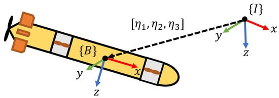
Figure 1.
The body-fixed frame and inertial frame .
3. AUV Control-Design Method
The control-design methods for AUVs vary in control objectives and controlled degrees of freedom (DoFs) depending on the available actuators and their configuration, but the general structure of all controlled AUV systems can be summarized by the block diagram in Figure 2. The controller consists of the control law that generates the total desired actuation from the desired state, and a control allocation method that determines how the total actuation is distributed between the available actuators. This mirrors the two components of the system model, with the actuator models producing the combined control actuation forces and moments, which then act on the AUV’s state based on its dynamics and kinematics. The sensors and observers in a controlled AUV system provide the controller with estimates of the system state, creating a closed control loop. Gyroscopes, inertial measurement units, and Doppler velocity logs are some of the common sensors used to obtain estimates of the vehicle’s velocities, position, and orientation. Kalman filters and other observer methods can be implemented to process the raw state readings from sensors and produce filtered state estimates that may not be directly measurable [5].
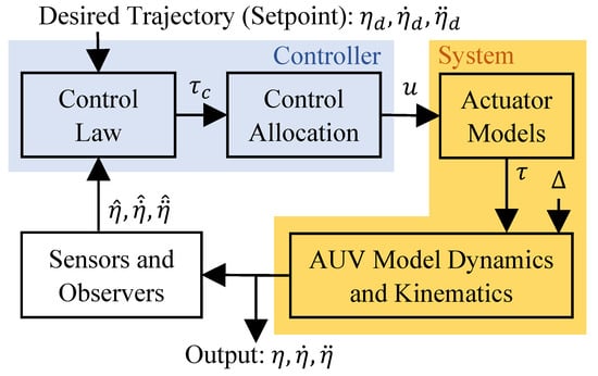
Figure 2.
The block diagram of a controlled AUV system.
Depending on the focus of a given work in the AUV control literature, assumptions are often made that further simplify this controlled system structure. Common assumptions for control design include ideal sensors () and ideal actuators (). When a fault occurs or when actuators are saturated, these assumptions are often violated. As surveyed in [34], a separate method from the control law is then needed to perform the control allocation for different actuator configurations. In this section, the AUV system and control objective are defined, followed by an initial control-law-design method.
3.1. System Configuration and Control Objective
Hybrid AUV configurations are equipped with control surfaces for efficient high-velocity maneuverability in underactuated conditions, and auxiliary thrusters for low-velocity maneuverability in fully actuated conditions. The actuator configuration used in this work is based on the the Delphin2 AUV used in [44]. For control actions in the vertical plane of motion, the system is equipped with two vertical auxiliary thrusters (front and aft), a pitch control surface, and a main thruster as shown in Figure 3.
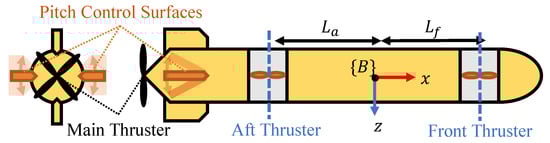
Figure 3.
The actuator configuration for the depth-pitch controlled AUV.
The control objectives are to track a desired trajectory ( and its derivatives) in the two DoFs that are of interest for this study (pitch and heave). The trajectory tracking is to be performed in both fully actuated and underactuated states, smoothly transitioning between low-speed hover-style control and high speed flight-style control. The auxiliary thruster forces and and the control-surface moment combine to produce to achieve the control objective, as shown later in Figure 4.
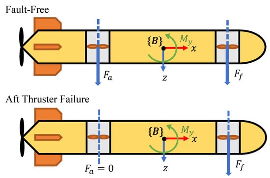
Figure 4.
The actuator forces and moments of the controlled system before and after the fault, with arrows indicating positive directions.
3.2. Model-Based PID Control Law
Though PID controllers have proven effective in controlling various complex systems such as unmanned aerial vehicles and robotic manipulators [45,46,47], the strong nonlinearities present in AUV systems make the direct application of a PID control-design method unsuitable. Instead, an estimate of the system model is incorporated into the control design to account for the system’s nonlinearities. Additional PID terms in the control law can then achieve the desired error dynamics.
The Fossen vectorial model for underwater vehicles was first described in [43] and has since been adopted for use in many AUV control-design methods. The model expresses the nonlinear dynamics and kinematics of an AUV for all six DoFs in the compact equations:
where the definitions of each variable are consistent with those found in Section 2.
When used for control design, the model is often simplified based on assumptions about the system to reduce the complexity of the design method. Some examples include the mass and hydrodynamics matrices being approximated as diagonal matrices, the Coriolis term being neglected, or the dimensions of the matrices and vectors being reduced to model fewer DoFs. For our AUV system, the values of these matrices are later specified in Section 5.
As a foundation for the actuator saturation and fault-tolerance techniques to be explored, we propose applying the model-based PID control law design method from [6] to our hybrid AUV configuration for depth-pitch trajectory tracking. The flexibility of the design method in [6] was demonstrated through applications on various systems, including the planar motion of a ship. The main contribution of the work in [6] was the development and proof of a constant disturbance estimation term using integral action. This includes the stability proof for the integral component, which is absent in other works on nonlinear PID controllers as it is far more complex than the same proof for linear PID control.
Proposition 1.
As detailed by the work in [6], a dynamic system described by the Equations (1) and (2) can track a desired trajectory using the control law:
where and its derivatives are the trajectory tracking errors. , and are user-defined positive definite diagonal gain matrices for tuning the controller. is an augmented reference velocity, and is an augmented velocity error.
The control law guarantees uniform global asymptotic stability and uniform local exponential stability in the presence of disturbance Δ by using the integral term . This term acts as an adaptive estimate of the unknown disturbances and is defined using:
where γ is a positive constant adaptation gain.
Proof.
Fossen’s model (1) can be expressed in the inertial frame’s coordinates using:
where the combined gravity and buoyancy term is considered as a component of the disturbance term , and each element has been transformed using :
These matrices still retain properties useful for control design. is positive diagonal, is strictly positive, and the resulting matrix of is skew-symmetric. This coordinate transformation enables the use of the model when considering a Lyapunov function based on the augmented velocity error s, which is in the inertial frame . Examining the Lyapunov candidate function:
where can be substituted using Equation (5) and the definition of s, such that:
Under the condition that , the use of the proposed control law (3) results in the Lyapunov candidate derivative:
From this point it is clear that without the disturbance and its compensation , the Lyapunov candidate derivative would be negative definite. As the extensive proof that converges to in this control law is prior literature, please refer to the original work by Fossen [6]. What is important to note is that with the disturbance compensation, the stability of the control law is proven to be uniform global asymptotic and uniform local exponential rather than uniform global exponential. □
As is common in the control law design literature, this control method was developed with the assumption that the system state (and its derivative ) can be accurately obtained. This assumption of ideal sensors is also applied to the propositions in the following section, where this control-design method is built upon with our fault-tolerance technique and saturation compensation terms. This results in the absence of the observer block from Figure 2 in the proposed controlled system diagram of Figure 5.
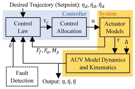
Figure 5.
The block diagram of the fault-tolerant and saturation-considerate system, considering the assumptions on ideal sensors for state estimation and fault detection.
4. Actuator-Fault and Saturation-Tolerance Methods
Fault compensation utilizes the remaining functional actuators to produce control forces/moments that offset any losses from a faulty actuator. A common technique is to re-allocate the forces and moments that were previously designated to the faulty actuator to other actuators that can produce outputs in the required direction. An issue occurs when the remaining actuators become saturated due to the reallocated forces/moments, which would then not be fully produced. Depending on the desired control and the amount of saturation, the system’s performance may degrade or become unstable even with fault compensation. To account for both faults and actuator saturation, the system’s actuator models and faulty states must be considered during control allocation.
4.1. Actuator Models
To account for actuator saturation and faults in both the controller and the system simulation, the actuators must be included in the system model. Taking advantage of the generalized form of Fossen’s vectorial model, which expresses the sum of all control forces and moments as , we can implement our own actuator models into the system model by specifying the composition of . The actuators of interest in our depth-pitch AUV system are the vertical auxiliary thrusters and the pitch control surface. For this work, we have simplified the actuator models so that instead of passing signals such as thruster voltage and control surface angle for each actuator, the actuators each receive allocated desired forces and moments in the vector u. Saturation limits on the range and rate of change of u are applied to determine the output thruster forces , and control-surface moment . This simplification is performed because each actuator is commonly equipped with its own micro-controller, which manages motor voltage to produce a desired rotational speed or angle that correlates with the produced force/moment. The actuator models used for the testing simulations will be described in Section 5.
4.2. Control Allocation
For control allocation, it is necessary to understand the relationship between individual actuator outputs and the total control forces and moments that act on the system. With our chosen actuator configuration for depth and pitch control, this relationship is described by the equation:
where and are the positive distances from the aft and front thrusters to frame , respectively, as seen in Figure 3.
From this equation, we can establish how the desired control should be allocated to the actuators. By updating this control allocation depending on actuator capabilities, the condition required by the control law can often be maintained even under actuator faults. Recalling the system structure block diagram shown in Figure 2, the generated by the PID control law is passed to the control allocation equation, which then passes the control signal u to the actuator models. In [6], the formula is used, where is the control allocation matrix calculated from pseudo-inverse of the AUV’s actuator configuration matrix B. The use of the actuator configuration matrix pseudo-inverse (Moore–Penrose inverse) for control allocation is also explored for underactuated and fully actuated underwater vehicle configurations [35,36,37,48]. For our controller, we replace the control allocation matrix with a dynamic term that is updated based on actuator faultiness, so that the pseudo-inverse operation is no longer used. This allows for more control flexibility than using the pseudo-inverse of the control configuration matrix.
For the faultless state, the following value is chosen such that the desired thrust is divided between the vertical thrusters to produce a total moment of zero. The desired moment is then generated by the control surface. Using an initial control allocation matrix:
we achieve the desired result for the hybrid AUV configuration. This holds true when there are no actuator faults and the elements of u are within their actuator limits and :
and substituting the elements of u as into (13):
4.3. Fault Compensation
To compensate for the effects of an actuator fault on the Lyapunov stability of a system, we must first understand how a fault changes the generated control forces/moments in . We examine two fault types: an aft-thruster failure (as shown in Figure 4) and control-surface failure .
As an example, examining the effects of an aft-thruster failure on our hybrid AUV configuration using the faultless state from (14), the total actuation becomes:
which invalidates the ideal actuator assumption . The stability from the Lyapunov analysis Equations (9)–(12) would then be uncertain unless the control allocation matrix is updated to consider the fault’s effects.
Proposition 2.
The dynamic control allocation matrix can be defined to compensate for the effects of the aft thruster or control-surface failure using:
where the value of δ refers to the detected fault state (0 = faultless, 1 = aft-thruster failure, and 2 = control-surface failure). The fault compensation maintains the stability condition during the occurrence of a fault, under the assumption that δ is estimated using a suitable fault-detection method (such as those reviewed in [22]) and that the allocated control signals u are within actuator saturation limits.
Proof.
When substituting for faulty actuation from (17) into the model-based PID controller’s Lyapunov analysis at (11), we find:
where the Lyapunov function is given by (9), and the control law for is given by (3). The stability of the system is now uncertain since the final term is not negative definite.
By modifying the control allocation of the desired forces and moments for the functioning front thruster and control surface using (18), the actuator output becomes:
which effectively compensates for the effects of aft-thruster failure by re-satisfying the Lyapunov proof condition for (12) that .
Similarly, a control-surface failure results in the faulty total actuator output:
resulting in the uncertain Lyapunov function derivative:
where the uncertain term is negated by updating the control allocation matrix for using (18):
□
Remark 1.
The fault-based switching occurs during control allocation and is separate from the control law. This maintains the control law’s stability during the control-allocation switching, assuming the fault detection is accurate. Other works have also suggested updating the control allocation matrix as a means of decoupling fault compensation from control law stability [24].
4.4. Saturation Compensation
When the values of u exceed the actuator limits, the condition is once again broken. Apart from faults, this can also occur due to large trajectory error terms in the controller. If this saturation is not taken into consideration by the controller, then the Lyapunov stability can become uncertain. However, if not all actuators are saturated then the control law can be designed to react to the control errors created by actuator saturation and retain stability at a slower transient response.
Proposition 3.
To develop a control law that accounts for actuator saturation, we choose a new Lyapunov function candidate:
where is a positive definite error function relating to the saturation of the individual actuators.
To provide a more controllable reaction to the presence of actuator saturation, the term is formulated as the following combination of exponential functions of the actuator outputs:
where λ is a positive parameter to control the sensitivity of the overall vehicle control when an actuator approaches saturation, and , , and are positive control parameters to set different emphasis on saturation avoidance for each actuator. It is assumed that estimates for the actuator outputs are observable. Note that when each actuator approaches its saturation state, its corresponding term is increased. Hence, the minimization of the term leads to saturation avoidance.
Proof.
By applying (26) to (25), the complete Lyapunov function candidate can now be written as:
where is the positive constant component of . This acts as the desired value for the saturation-based terms, which offsets the function’s global minimum to zero, producing a positive definite :
If the Lyapunov candidate function’s derivative is negative definite, then the saturation terms in (27) must approach zero. □
Remark 2.
A key characteristic of a Lyapunov function is its positive definiteness. This ensures that its only point of stability is located at the origin, where all the equation’s parameters (which are error values) are zero. In the extra term added to the Lyapunov function, the actuator outputs are used as parameters instead of some saturation error based on the desired actuator outputs such as . Although the actuator outputs do not necessarily have a desired value of zero like the error values used in , the choice to use the actuator outputs like directly as a parameter in simplifies the derivatives of and hence the control law selection process. The choice of and its parameters enables the saturation-based terms to take effect when approaching saturation while being otherwise negligible without breaking the positive definiteness of the function.
4.5. Proposed Controller
To apply the described saturation and fault tolerance, we propose a controller with the objective of trajectory tracking in the heave and pitch DoFs, for the actuator configuration shown in Figure 3. The controller must be able to operate in both low- and high-velocity trajectories while maintaining stability and maximizing the transient response of the trajectory tracking when the system is faced with actuator faults and saturation.
Theorem 1.
Based on Propositions 2 and 3 regarding the hybrid AUV and control objectives specified in Section 3.1, the control law:
makes the derivative of the Lyapunov candidate (27) negative definite. This guarantees asymptotic stability through convergence of and s towards zero while driving the actuator control signals away from their saturation limits. When used with the dynamic control allocation matrix defined by (18), control stability is maintained in the presence of actuator faults (aft-thruster failure or control-surface failure) and control performance is maintained by minimizing the effects of actuator saturation. This holds true under the assumptions that estimates can be obtained for:
- the fault state δ used in (18) for actuator fault compensation
- the actuator outputs for actuator saturation tolerance
Additionally, the control law’s sensitivity to actuator saturation estimates are explored in Appendix A.
Proof.
By choosing as (30) for a system not experiencing actuator saturation and using dynamic control allocation from proposition 1 to compensate for actuator faults, becomes a negative definite function:
which guarantees the asymptotic stability of the error terms and s about zero while driving the actuator control signals (and hence the actuator outputs) away from the actuator limits.
Although the control gains , and can be chosen such that the saturation terms in the control law prevents actuator saturation, sudden external disturbances or faults may still result in saturation. For these cases, let us examine the Lyapunov function’s derivative (32) when experiences actuator saturation. During saturation, let us define an actuation error as:
and use it in the Lyapunov derivative (32) to find:
Given that the low frequency of is similar to that of , it behaves similarly to the unknown disturbance forces and torques and will be compensated for by the adaptive term . □
The final system block diagram, which uses the actuator readings to consider actuator saturation in the control law, is visualized in Figure 5.
Remark 3.
The proposed design method of including the saturation-based terms to a model-based control law with proven Lyapunov stability can be applied to any underwater vehicle actuator configuration. This flexibility is made possible by Fossen’s model, which considers all six DoFs, and the control allocation being separate from the control law such that it can be re-selected for each actuator configuration or possible fault. The fault-compensation method itself can also be replaced by more advanced methods (active observer-based methods or passive robust/adaptive methods) and still benefit from the saturation compensation.
5. Simulation Setup and Results
To demonstrate the proposed control method’s ability to improve trajectory tracking in the presence of faults, two controlled systems were simulated on a trajectory with varying fault conditions for comparison. Fossen’s vectorial model and our actuator models were used to simulate the hybrid AUV configuration when controlled with either the proposed fault and saturation-tolerant controller from Theorem 1 or the baseline controller to be described in Section 5.1. The system parameters used for these simulations are presented in Table 2, some of which are model parameters extracted from the AUV system described in [49]. The gain values used in the controller were obtained through trial and error, with the initial values and the choice of force-to-moment ratio based on the control values used for the same AUV model parameters in [49]. The values relating to the other four DoFs have been set to zero because the controllers have been designed for the heave and pitch DoFs, while the simulation considers all six DoFs.
Table 2.
Simulation parameters.
These simulations are performed assuming the use of ideal sensors, with the state values used in the controller being directly obtained from the system model. The actuator models used in these simulations consist of limits ( and for the forces and moments, respectively) that constrain the control value to within an actuator’s capabilities, and transfer functions that serve as the rate limits for the actuators. These models are defined using:
Remark 4.
The time constants used for (39) differ from those in (37) and (38) since the control surface has different limits on its output’s derivative compared to the limits for the auxiliary thrusters.
Remark 5.
Equation (36) incorporates the actuator saturation limits with the assumption that the actuator performances are symmetrical about zero. Although this assumption is true for the actuators in the proposed configuration (auxiliary tunnel thrusters and pitch control surfaces), it may not hold true for other actuator configurations. For such configurations, the actuator model equations can be modified for asymmetric saturation limits.
5.1. Baseline Controller
To enable comparisons with the proposed controller, we present a baseline controller using the design method described in Section 3.2. The baseline controller’s objectives are the same as the proposed controller, described in Section 3.1. The controller is paired with the control allocation described by (14) for the actuator configuration shown in Figure 3 in a faultless state, to perform the trajectory tracking in both low- and high-velocity trajectories by transitioning between hover and flight style control.
5.2. Simulation Conditions
The simulations are conducted using a simple trajectory: an initial position [0;0;0;0;0;0] that translates to the constant position [0;0;50;0;0;0] in 5 s. This trajectory is practically equivalent to the set point used by other control methods, except for the initial ramp in depth that is set by the trajectory instead of being dictated by the controller. This trajectory was chosen with the purpose of investigating the transient responses of the controllers, with the initial high velocity ensuring that the baseline control law would push the thrusters to saturation. This provides a controlled situation for observing how the proposed controller reacts to the saturation.
The simulations were conducted in the absence of a disturbance force since robustness to external disturbances has been well explored in the literature and may detract from this work’s focus on actuator faults and saturation. Running the simulations without disturbances also allows for the effectiveness of the saturation compensation against the chosen fault to be directly assessed. The performance of the controlled systems is compared using the settling times of the depth error (when within m of zero) and the pitch error (when within degrees of zero), as well as the peak values of these errors after a fault occurs and the root mean square (RMS) error in depth and pitch.
5.3. Baseline System Performance
To form a basis for the performance of the proposed fault and saturation-tolerant controller, we begin by simulating the system using the baseline model-based PID controller. The system is simulated performing the trajectory under three conditions: without faults, with aft-thruster failure occurring at s, and with a control-surface failure occurring at s. These fault timings were chosen to ensure that the failing actuators were active as the chosen faults would have no effect on an actuator with a desired output of zero. The resulting tracking performance and actuator outputs are shown in Figure 6 and Figure 7, respectively.
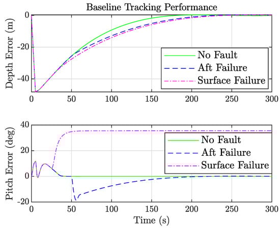
Figure 6.
Depth and pitch errors for the baseline controller under the three conditions; faultless, aft failure at s, and control-surface failure at s.
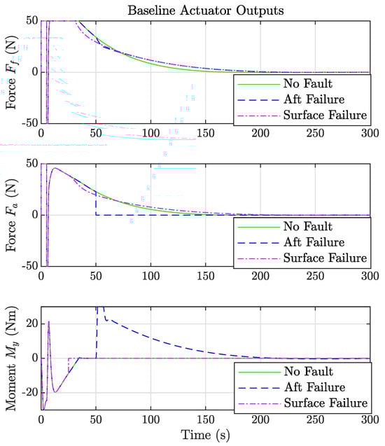
Figure 7.
Actuator outputs for the baseline controller under the three conditions; faultless, aft failure at s, and control-surface failure at s.
5.4. Proposed System Performance
Next, we simulate the proposed saturation and fault-tolerant controller for aft-thruster failure and control-surface failure. The results for these systems performing under the previously described trajectory and fault states are overlaid with results for the baseline PID in the same simulation conditions and are shown in Figure 8, Figure 9, Figure 10 and Figure 11.
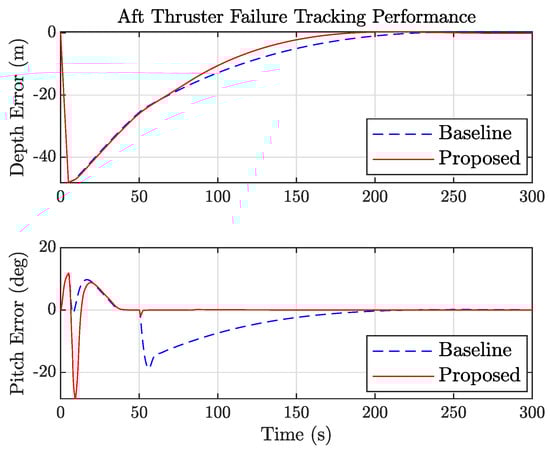
Figure 8.
Depth and pitch errors over time for the baseline and proposed saturation and fault-tolerant controllers under aft-thruster failure at s.
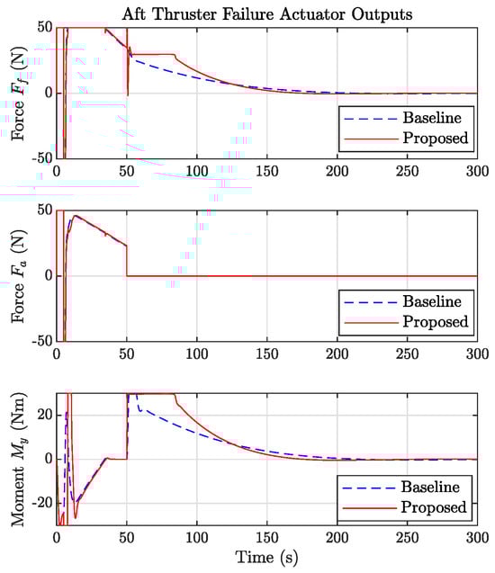
Figure 9.
Actuator outputs over time for the baseline and proposed saturation and fault-tolerant controllers under aft-thruster failure at s.
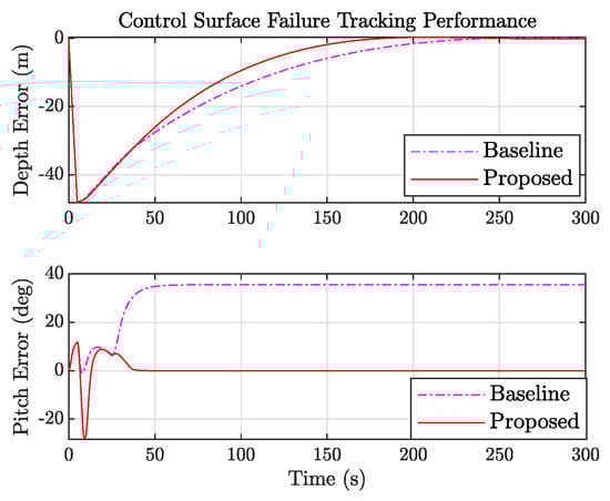
Figure 10.
Depth and pitch errors over time for the baseline and proposed saturation and fault-tolerant controllers under control-surface failure at s.
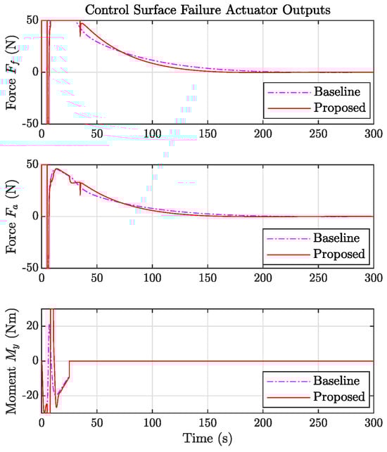
Figure 11.
Actuator outputs over time for the baseline and proposed saturation and fault-tolerant controllers under control-surface failure at s.
The quantified tracking performance for these simulations is summarized in Table 3 and Table 4, highlighting the improved performance of the proposed controller over the baseline controller. For both fault types, the proposed system improves on the settling time, post-fault peaks, and RMS of the depth and pitch errors.
Table 3.
System performance: aft-thruster failure.
Table 4.
System performance: control-surface failure.
6. Discussion
There are a few notable features in the tracking performance and actuator output graphs that are common between all of the simulations of the baseline system. The initial high velocity of the desired trajectory is evident in Figure 6 from the rapidly ramping depth error in the first five seconds, which then peaks once the desired trajectory reaches its specified depth. During this time, both thrusters are saturated as the depth error increases the desired control thrust, up to the point where the desired trajectory suddenly halts. This large discontinuity in the desired velocity dominates the depth error in the control law, causing the sharp peaks seen in all actuators in Figure 7 at about five seconds. The last common features are the two humps in the pitch error at the beginning of the simulation, shown in Figure 6. These are caused by the unaccounted moment from the imbalanced thrusters that are saturated during that time. The initial peak in the control-surface moment is then a reaction to this pitch error.
6.1. Fault Effects on the Baseline-Controller Stability
Examining the errors in Figure 6 for the baseline controller under aft-thruster and control-surface failures, we see that while both faults cause an increase in the depth-error settling time compared to the simulation without faults; only the control-surface failure prevents the convergence of the pitch error to zero. The thruster failure does not prevent the baseline controller from re-settling the pitch error at approximately zero. As seen in the actuator output graphs in Figure 7, this is because the unaccounted moment produced by the thruster failure is still compensated for by the control-surface moment in the reaction to the pitch error. In the case where the control surface fails instead, the two remaining thrusters do not compensate for the unaccounted lost-control moment when using the baseline controller’s control allocation.
6.2. Controller Fault-Response Comparison
Before the occurrence of the faults in both faulty state simulations seen in Figure 9 and Figure 10, we note that the proposed controller’s initial pitch-error peak is much larger than that seen in the baseline controller. As shown in Table 3 and Table 4, the pre-fault pitch errors of the proposed controller are approximately 2.4 times the error values of the baseline controller. This can be attributed to the large actuator output derivatives during this time, which cause the control moment to prioritize compensating for the saturated thrusters over reducing the pitch or velocity errors. Soon after, the pitch-error peaks subside and converge with the baseline controller values until the faults occur. These increased peaks can be avoided by selecting a smooth desired trajectory.
Upon aft-thruster failure, we see that the fault compensation causes both remaining actuator outputs to peak in Figure 9, though the saturation compensation then quickly drives the front thrust downward before it plateaus for the remainder of the control surface’s saturation. These actions quickly settle the pitch error seen in Figure 8, reducing both its settling time and post-fault peak magnitude shown in Table 3. The reduced pitch error then maintains a larger component of the thrust force facing toward the desired depth, which improves the depth-error settling time.
In the control-surface failure simulations, we see in Figure 11 that the fault tolerance causes the aft thrust to plateau at a lower value after the fault. Figure 10 shows that the thruster imbalance then corrects the pitch error, improving its settling time. The saturation terms cause a small peak in the thrusts after this plateau. Again, the reduced pitch error enables the thrusters to improve the depth-error settling time listed in Table 4.
6.3. Limitations of the Proposed Controller and Simulations
As an initial investigation on the utility of saturation-based control law terms coupled with fault-tolerant control allocation, the proposed control-design method is currently limited in applicability. Though this limitation is not unique to the proposed controller, the control law assumes the availability of system and actuator states for use in the controller. Solutions for actuator output estimation exist but have not been explored by the literature to the same extent as position and velocity estimation, and actuator fault classification for underwater vehicles. The current method is also specific to the actuator configuration and chosen DoFs (heave and pitch). Though the method is flexible enough to be adapted to other configurations and DoF ranges, the effectiveness of the saturation terms in these applications will need to be investigated. The choice of is also currently based on expert knowledge of the actuator configuration and may be substituted with other control allocation methods under less faulty actuator conditions.
The simulations used to quantify the performance of the proposed controller are also limited, specifically by the accuracy of the Fossen system model, the actuator models, and the exclusion of external disturbances. Ideally, the performance of all controllers would be determined through physical system experiments to expose the controller to all the unmodelled dynamics. Further simulations with different trajectories may also reveal more information regarding the effectiveness of the saturation terms and control allocation and would be necessary if the proposed method is extended to more DoFs.
6.4. Comparison to Existing Techniques
The direct quantitative comparison of our controller’s performance with the results of other existing AUV control methods would require the application of both methods to the same AUV system and trajectory, similar to what was performed with the baseline controller. However, the fault- and saturation-tolerance techniques can be compared in terms of applicability and assumptions.
Three works propose fault-tolerant control allocation methods for AUVs [37,38,39]. In [37], three types of DoF (surge, sway, and yaw) horizontal planar control are considered. The actuator configuration consists of four thrusters—one on each corner of the box-shaped vehicle. To perform fault compensation, a diagonal weight matrix W is introduced to the control allocation:
which uses the Moore–Penrose pseudo-inverse operation. The elements of the diagonal matrix correspond to the faultiness of each actuator, with values between one (faultless) and zero (complete failure). It is stated that using this control allocation provides the optimal solution in a faultless state, the unique solution when one thruster fails, and the least squares solution when two or more thrusters fail. The work also proposes an equivalent “virtual thruster” method for the specific four-thruster actuator configuration for the case of single thruster failure.
The work in [38] considered another thruster-based configuration, with four thrusters all placed on the aft of a cylindrical hull. The work proposes an alternative to the pseudo-inverse for faultless control allocation, due to its computational complexity. The proposed method relies on the configuration matrix fulfilling two properties: that its rows are mutually orthogonal, and that B can be separated into a diagonal matrix and a row-orthogonal matrix , whose entries are either or such that . The work proposed the configuration-specific control allocation formula:
where . For the fault compensation of a single thruster failure, another alternative to the pseudo-inverse is proposed. The work defined , where the element corresponding to the failed thruster is removed from u, and , where the column corresponding to the failed thruster is removed from R. The control allocation for the functional thrusters is then calculated using:
Similar to these two works, our proposed control allocation method is specific to the considered actuator configuration. To the authors’ knowledge, there is no other literature on the control allocation for the hybrid configuration described in Section 3.1. Our proposed control allocation also utilitizes fault-specific allocation matrices as performed in [38] rather than calculating a pseudo-inverse based on all thruster fault conditions as carried out in [37]. The use of per-fault matrices also removes the need for quantitative fault detection, which makes the assumption of fault detection availability more achievable. Unlike these two works, we consider the actuator saturation that becomes more likely due to distributing the control over fewer actuators.
The only other work that the authors are aware of that considers actuator saturation in fault-tolerant control allocation is [39]. The actuator configuration considered by the work consists of a spherical hull with eight thrusters. Two thrusters attached on opposite sides of the sphere form a pair that produce surge forces, and a similar pair produce sway forces. The two pairs can also produce a yaw moment as they are attached on the same horizontal plane. Four more thrusters that point vertically to produce heave forces, roll moments, and pitch moments are attached at the same points of the two thruster pairs. For the fault-tolerant control allocation, a weighted pseudo-inverse of the configuration matrix is used, as seen in [37]. To address thruster saturation, the work proposed a dynamic state feedback technique. This involved using the control allocation u as part of the system state, which was estimated using an integral term. The estimate of u is then used to calculate a diagonal weight matrix whose elements are when the corresponding thruster is in the middle of the saturation range and to approach infinity towards saturation. Using the inverse of this weight matrix in the control allocation reduces the change in u as an actuator approaches saturation.
In comparison, our proposed method of handling actuator saturation is implemented separately from the control allocation. This choice was made considering that actuator saturation is often handled in the control law as part of disturbance and uncertainty estimation. This simplifies the substitution of the saturation compensation technique with others in existing control laws. The saturation terms in both our work and [39] perform saturation compensation through the reduction in allocated control to saturating actuators; however, our proposed control-law method reacts to saturation by reducing the desired control relative to the augmented velocity error s. An implementation of saturation compensation through control allocation for the hybrid AUV configuration should also be considered in future work.
7. Conclusions
Robust control systems are a necessity for AUV systems due to the control model discrepancies that can be caused by environmental uncertainties, model parameter simplification, and actuator faults. Motivated by the benefits of hybrid AUV actuator configurations, we propose the use of nonlinear control law terms for actuator saturation tolerance, and a fault-tolerant control allocation method for a hybrid AUV configuration. A controller is implemented for trajectory tracking in the heave and pitch DoFs and is simulated under two types of actuator faults: aft-thruster failure and control-surface failure. Comparing the simulation results with simulations using a baseline controller demonstrates how the proposed control methods can produce improved performance in terms of the tracking error settling times. In collision-prone operations, this improvement may prevent further damage to the system or its surroundings in the case of an actuator failure.
This work can be taken further to increase the applicability of the actuator saturation and fault-tolerant control design. This can be achieved by extending the design method to consider more DoFs, and by deriving gain tuning conditions based on a system’s state and trajectory limits. The design methods can also be implemented on top of other base-controller types such as sliding mode control, and other control allocation methods from the literature. The utility of the combined methods should be compared with other saturation and fault-tolerance techniques such as optimization control and adaptive control to solidify the effectiveness of the proposed method. The simulations used to determine the performance of a controller designed using the proposed method should also be improved with higher fidelity actuator and system models (including sensor and observer implementations) and be validated through tests using a physical system.
Supplementary Materials
The following supporting information can be downloaded at: https://www.mdpi.com/article/10.3390/electronics12214495/s1.
Author Contributions
Conceptualization, X.M. and R.H.; methodology, X.M. and R.H.; software, X.M. and R.H.; validation, X.M.; formal analysis, X.M.; investigation, X.M.; data curation, X.M.; writing—original draft preparation, X.M.; writing—review and editing, R.H., A.F., S.K. and A.B.-H.; visualization, X.M.; supervision, R.H., A.F. and A.B.-H.; and project administration, A.B.-H. All authors have read and agreed to the published version of the manuscript.
Funding
This research received no external funding.
Data Availability Statement
The data presented in this study are available in the Supplementary Materials.
Acknowledgments
During the development of this work, X. Macatangay received support from RMIT University through scholarships, including an Australian Government Research Training Program (RTP) Scholarship.
Conflicts of Interest
The authors declare no conflict of interest. The funders had no role in the design of the study; in the collection, analyses, or interpretation of data; in the writing of the manuscript; or in the decision to publish the results.
Abbreviations
The following abbreviations are used in this manuscript:
| AUV | Autonomous underwater vehicle |
| DoF | Degree of freedom |
| PID | Proportional integral derivative |
| RMS | Root mean square |
Appendix A. State Error Sensitivity
The proposed control law is developed assuming that sensors or observers accurately estimate the actuator outputs and , as explored in [50]. To determine the impact of inaccuracies on the values returned by sensors or observers for actuator outputs, an analysis of the sensitivity of the saturation terms included in the proposed control law, to any changes/inaccuracy in the actuator outputs, is presented. The sensitivity analysis is conducted by obtaining the ratio between small changes of output and input for:
where z is the generalized form of the saturation terms found in (30). We begin by defining:
so that z can be rewritten as:
Taking the partial derivative in terms of F we find:
Noting that:
the partial derivative can be rewritten as:
leading to the final sensitivity of:
Therefore, the effect of an actuator output measurement error increases from a 1:1 ratio to the function z at a quadratic rate relative to the actual actuator output value. It should be noted that this analysis does not consider the relative magnitude of z to , which is affected by .
References
- Wynn, R.B.; Huvenne, V.A.; Le Bas, T.P.; Murton, B.J.; Connelly, D.P.; Bett, B.J.; Ruhl, H.A.; Morris, K.J.; Peakall, J.; Parsons, D.R.; et al. Autonomous Underwater Vehicles (AUVs): Their past, present and future contributions to the advancement of marine geoscience. Mar. Geol. 2014, 352, 451–468. [Google Scholar] [CrossRef]
- Hover, F.S.; Eustice, R.M.; Kim, A.; Englot, B.; Johannsson, H.; Kaess, M.; Leonard, J.J. Advanced perception, navigation and planning for autonomous in-water ship hull inspection. Int. J. Robot. Res. 2012, 31, 1445–1464. [Google Scholar] [CrossRef]
- Bogue, R. Underwater robots: A review of technologies and applications. Ind. Robot. 2015, 42, 186–191. [Google Scholar] [CrossRef]
- Mat-Noh, M.; Arshad, M.R.; Md Zain, Z.; Khan, Q. Review of sliding mode control applications in autonomous underwater vehicles. Indian J. Geo-Mar. Sci. 2019, 48, 973–984. [Google Scholar]
- Fossen, T.I. Handbook of Marine Craft Hydrodynamics and Motion Control; Wiley: Chichester, UK, 2011. [Google Scholar]
- Fossen, T.I.; Loría, A.; Teel, A. A theorem for UGAS and ULES of (passive) nonautonomous systems: Robust control of mechanical systems and ships. Int. J. Robust Nonlinear Control. 2001, 11, 95–108. [Google Scholar] [CrossRef]
- Mirzaei, M.; Taghvaei, H. A Full Hydrodynamic Consideration in Control System Performance Analysis for an Autonomous Underwater Vehicle. J. Intell. Robot. Syst. 2020, 99, 129–145. [Google Scholar] [CrossRef]
- Shi, Y.; Shen, C.; Fang, H.; Li, H. Advanced Control in Marine Mechatronic Systems: A Survey. IEEE/ASME Trans. Mechatronics 2017, 22, 1121–1131. [Google Scholar] [CrossRef]
- Khalid, M.U.; Ahsan, M.; Kamal, O.; Najeeb, U. Modeling and Trajectory Tracking of Remotely Operated Underwater Vehicle using Higher Order Sliding Mode Control. In Proceedings of the 2019 16th International Bhurban Conference on Applied Sciences and Technology (IBCAST), Islamabad, Pakistan, 8–12 January 2019; pp. 855–860. [Google Scholar]
- Ismail, Z.H.; Putranti, V.W.E. Second Order Sliding Mode Control Scheme for an Autonomous Underwater Vehicle with Dynamic Region Concept. Math. Probl. Eng. 2015, 2015, 1–13. [Google Scholar] [CrossRef]
- Perez, T.; Donaire, A.; Renton, C.; Valentinis, F. Energy-based Motion Control of Marine Vehicles using Interconnection and Damping Assignment Passivity-based Control—A Survey. IFAC Proc. Vol. 2013, 46, 316–327. [Google Scholar] [CrossRef]
- García, D.; Sandoval, J.; Gutiérrez–Jagüey, J.; Bugarin, E. IDA-PBC Control of an Underactuated Underwater Vehicle. Rev. Iberoam. Autom. Inform. Ind. 2017, 15, 36–45. [Google Scholar] [CrossRef]
- Jia, Z.; Qiao, L.; Zhang, W. Adaptive tracking control of unmanned underwater vehicles with compensation for external perturbations and uncertainties using Port-Hamiltonian theory. Ocean Eng. 2020, 209, 107402. [Google Scholar] [CrossRef]
- Antonelli, G.; Caccavale, F.; Chiaverini, S.; Fusco, G. A novel adaptive control law for underwater vehicles. IEEE Trans. Control. Syst. Technol. 2003, 11, 221–232. [Google Scholar] [CrossRef]
- Yu, C.; Zhong, Y.; Lian, L.; Xiang, X. An experimental study of adaptive bounded depth control for underwater vehicles subject to thruster’s dead-zone and saturation. Appl. Ocean Res. 2021, 117, 102947. [Google Scholar] [CrossRef]
- Antonelli, G.; Chiaverini, S.; Sarkar, N.; West, M. Adaptive control of an autonomous underwater vehicle: Experimental results on ODIN. IEEE Trans. Control. Syst. Technol. 2001, 9, 756–765. [Google Scholar] [CrossRef]
- Tijjani, A.S.; Chemori, A.; Creuze, V. Robust Adaptive Tracking Control of Underwater Vehicles: Design, Stability Analysis, and Experiments. IEEE/ASME Trans. Mechatronics 2021, 26, 897–907. [Google Scholar] [CrossRef]
- Dong, B.; Shi, Y.; Xie, W.; Chen, W.; Zhang, W. Learning-based robust optimal tracking controller design for unmanned underwater vehicles with full-state and input constraints. Ocean Eng. 2023, 271, 113757. [Google Scholar] [CrossRef]
- Heshmati-Alamdari, S.; Karras, G.C.; Marantos, P.; Kyriakopoulos, K.J. A Robust Predictive Control Approach for Underwater Robotic Vehicles. IEEE Trans. Control. Syst. Technol. 2020, 28, 2352–2363. [Google Scholar] [CrossRef]
- Xia, Y.; Xu, K.; Wang, W.; Xu, G.; Xiang, X.; Li, Y. Optimal robust trajectory tracking control of a X-rudder AUV with velocity sensor failures and uncertainties. Ocean Eng. 2020, 198, 106949. [Google Scholar] [CrossRef]
- Antonelli, G. A survey of fault detection/tolerance strategies for AUVs and ROVs. In Fault Diagnosis and Fault Tolerance for Mechatronic Systems: Recent Advances; Springer: Berlin/Heidelberg, Germany, 2003; pp. 109–127. [Google Scholar]
- Liu, F.; Tang, H.; Qin, Y.; Duan, C.; Luo, J.; Pu, H. Review on fault diagnosis of unmanned underwater vehicles. Ocean Eng. 2022, 243, 110290. [Google Scholar] [CrossRef]
- Zhao, B.; Skjetne, R.; Blanke, M.; Dukan, F. Particle Filter for Fault Diagnosis and Robust Navigation of Underwater Robot. IEEE Trans. Control. Syst. Technol. 2014, 22, 2399–2407. [Google Scholar] [CrossRef]
- Baldini, A.; Felicetti, R.; Freddi, A.; Longhi, S.; Monteriu, A.; Fasano, A. Fault Detection, Diagnosis and Fault Tolerant Output Control for a Remotely Operated Vehicle. In Proceedings of the 2018 14th IEEE/ASME International Conference on Mechatronic and Embedded Systems and Applications (MESA), Oulu, Finland, 2–4 July 2018; pp. 1–7. [Google Scholar]
- Liu, X.; Zhang, M.; Wang, Y.; Rogers, E. Design and Experimental Validation of an Adaptive Sliding Mode Observer-Based Fault-Tolerant Control for Underwater Vehicles. IEEE Trans. Control. Syst. Technol. 2019, 27, 2655–2662. [Google Scholar] [CrossRef]
- Wang, X.; Tan, C.P. Dynamic Output Feedback Fault Tolerant Control for Unmanned Underwater Vehicles. IEEE Trans. Veh. Technol. 2020, 69, 3693–3702. [Google Scholar] [CrossRef]
- Corradini, M.L.; Monteriu, A.; Orlando, G. An Actuator Failure Tolerant Control Scheme for an Underwater Remotely Operated Vehicle. IEEE Trans. Control. Syst. Technol. 2011, 19, 1036–1046. [Google Scholar] [CrossRef]
- Hu, T.; Lin, Z. Control Systems with Actuator Saturation: Analysis and Design; Springer Science & Business Media: Berlin/Heidelberg, Germany, 2001. [Google Scholar]
- Guerrero, J.; Torres, J.; Creuze, V.; Chemori, A.; Campos, E. Saturation based nonlinear PID control for underwater vehicles: Design, stability analysis and experiments. Mechatronics 2019, 61, 96–105. [Google Scholar] [CrossRef]
- Hasan, M.W.; Abbas, N.H. Disturbance Rejection for Underwater robotic vehicle based on adaptive fuzzy with nonlinear PID controller. ISA Trans. 2022, 130, 360–376. [Google Scholar] [CrossRef]
- Shen, C.; Shi, Y. NMPC Design for AUV Dynamic Positioning Control with Incremental Input Constraints. In Proceedings of the 2022 IEEE 5th International Conference on Industrial Cyber-Physical Systems (ICPS), Coventry, UK, 24–26 May 2022; pp. 1–6. [Google Scholar] [CrossRef]
- Nioras, A.; Karras, G.C.; Fourlas, G.K.; Stamoulis, G. Survey of fault diagnosis and accommodation of unmanned underwater vehicles. In Proceedings of the CEUR Workshop Proceedings, Warsaw, Poland, 27–30 August 2018; Volume 2289. [Google Scholar]
- Kostenko, V.V.; Tolstonogov, A.Y. A comparative analysis of control allocation methods applied to autonomous underwater vehicles. J. Phys. Conf. Ser. 2021, 1864, 012145. [Google Scholar] [CrossRef]
- Fossen, T.I.; Johansen, T.A. A Survey of Control Allocation Methods for Ships and Underwater Vehicles. In Proceedings of the 2006 14th Mediterranean Conference on Control and Automation, Ancona, Italy, 28–30 June 2006; pp. 1–6. [Google Scholar] [CrossRef]
- Chen, Y.Y.; Lee, C.Y.; Huang, Y.X.; Yu, T.T. Control Allocation Design for Torpedo-like Underwater Vehicles with Multiple Actuators. Actuators 2022, 11, 104. [Google Scholar] [CrossRef]
- Zhang, Y.; Li, Y.; Zhang, G.; Zeng, J.; Wan, L. Design of X-rudder autonomous underwater vehicle’s quadruple-rudder allocation with Lévy flight character. Int. J. Adv. Robot. Syst. 2017, 14, 1729881417741738. [Google Scholar] [CrossRef]
- Fasano, A.; Ferracuti, F.; Freddi, A.; Longhi, S.; Monteriù, A. A Virtual Thruster-Based Failure Tolerant Control Scheme for Underwater Vehicle. IFAC-PapersOnLine 2015, 48, 146–151. [Google Scholar] [CrossRef]
- Garus, J.; Studanski, R.; Batur, T. Passive fault-tolerant control allocation for small unmanned underwater vehicle. J. Mar. Eng. Technol. 2017, 16, 420–424. [Google Scholar] [CrossRef][Green Version]
- Sarkar, N.; Podder, T.; Antonelli, G. Fault-accommodating thruster force allocation of an AUV considering thruster redundancy and saturation. IEEE Trans. Robot. Autom. 2002, 18, 223–233. [Google Scholar] [CrossRef]
- Packard, G.E.; Stokey, R.; Christenson, R.; Jaffre, F.; Purcell, M.; Littlefield, R. Hull inspection and confined area search capabilities of REMUS autonomous underwater vehicle. In Proceedings of the OCEANS 2010 MTS/IEEE SEATTLE, Seattle, WA, USA, 20–23 September 2010; pp. 1–4. [Google Scholar]
- Steenson, L.V.; Turnock, S.R.; Phillips, A.B.; Harris, C.; Furlong, M.E.; Rogers, E.; Wang, L.; Bodles, K.; Evans, D.W. Model predictive control of a hybrid autonomous underwater vehicle with experimental verification. Proc. Inst. Mech. Eng. Part J. Eng. Marit. Environ. 2014, 228, 166–179. [Google Scholar] [CrossRef]
- Caiti, A.; Di Corato, F.; Fenucci, D.; Grechi, S.; Novi, M.; Pacini, F.; Paoli, G. The project V-fides: A new generation AUV for deep underwater exploration, operation and monitoring. In Proceedings of the 2014 Oceans—St. John’s, St. John’s, NL, Canada, 14–19 September 2014; pp. 1–7. [Google Scholar]
- Fossen, T.I. Nonlinear Modelling and Control of Underwater Vehicles. Master’s Thesis, Universitetet i Trondheim, Trondheim, Norway, 1991. [Google Scholar]
- Tanakitkorn, K.; Wilson, P.A.; Turnock, S.R.; Phillips, A.B. Depth control for an over-actuated, hover-capable autonomous underwater vehicle with experimental verification. Mechatronics 2017, 41, 67–81. [Google Scholar] [CrossRef]
- Liu, L. Design of UAV Flight Control Law Based on PID Control. In Proceedings of the 2021 International Conference on Signal Processing and Machine Learning (CONF-SPML), Stanford, CA, USA, 14 November 2021; pp. 98–101. [Google Scholar] [CrossRef]
- Chen, W.H.; Chen, J.I.Z. Performance Evaluation of a Quadcopter by an Optimized PID. In Proceedings of the 2023 Sixth International Symposium on Computer, Consumer and Control (IS3C), Taichung, Taiwan, 30 June–3 July 2023; pp. 288–291. [Google Scholar] [CrossRef]
- Borase, R.P.; Maghade, D.K.; Sondkar, S.Y.; Pawar, S.N. A review of PID control, tuning methods and applications. Int. J. Dyn. Control 2021, 9, 818–827. [Google Scholar] [CrossRef]
- Baldini, A.; Ciabattoni, L.; Felicetti, R.; Ferracuti, F.; Freddi, A.; Monteriù, A. Dynamic surface fault tolerant control for underwater remotely operated vehicles. ISA Trans. 2018, 78, 10–20. [Google Scholar] [CrossRef] [PubMed]
- Nguyen, L.H.; Hua, M.D.; Hamel, T. A nonlinear control approach for trajectory tracking of slender-body axisymmetric underactuated underwater vehicles. In Proceedings of the 2019 18th European Control Conference (ECC), Naples, Italy, 25–28 June 2019; pp. 4053–4060. [Google Scholar] [CrossRef]
- Pivano, L. Thrust Estimation and Control of Marine Propellers in Four-Quadrant Operations. Ph.D. Thesis, NTNU—Faculty of Information Technology, Mathematics and Electrical Engineering, Trondheim, Norway, 2008. [Google Scholar]
Disclaimer/Publisher’s Note: The statements, opinions and data contained in all publications are solely those of the individual author(s) and contributor(s) and not of MDPI and/or the editor(s). MDPI and/or the editor(s) disclaim responsibility for any injury to people or property resulting from any ideas, methods, instructions or products referred to in the content. |
© 2023 by the authors. Licensee MDPI, Basel, Switzerland. This article is an open access article distributed under the terms and conditions of the Creative Commons Attribution (CC BY) license (https://creativecommons.org/licenses/by/4.0/).