Abstract
In order to improve the safety and efficiency of inspection robots for solar power plants, the Rapidly Exploring Random Tree Star (RRT*) algorithm is studied and an improved method based on an adaptive target bias and heuristic circular sampling is proposed. Firstly, in response to the problem of slow search speed caused by random samplings in the traditional RRT* algorithm, an adaptive target bias function is applied to adjust the generation of sampling points in real-time, which continuously expands the random tree towards the target point. Secondly, to solve the problem that the RRT* algorithm has a low search efficiency and stability in narrow and long channels of solar power plants, the strategy of heuristic circular sampling combined with directional deviation is designed to resample nodes located on obstacles to generate more valid nodes. Then, considering the turning range of the inspection robot, our method will prune nodes on the paths that fail to meet constraint of the minimum turning radius. Finally, the B-spline curve is used to fit and smooth the path. A simulation experiment based on the environment of solar power plant is conducted and the result demonstrates that, compared with the RRT*, the improved RRT* algorithm reduces the search time, iterations, and path cost by 62.06%, 45.17%, and 1.6%, respectively, which provides a theoretical basis for improving the operational efficiency of inspection robots for solar power plants.
1. Introduction
With the rapid growth of clean energy demand, especially photovoltaic (PV) generation, the number of solar power plants has been increasing year by year and has reached a larger scale [1,2,3]. The fault detection work of solar power plants is also developing towards automation and unmanned direction, while traditional manual detection work is gradually being replaced by unmanned aerial vehicles (UAV) and inspection robots [4,5,6]. The widespread application of UAV and inspection robots has remarkably reduced the working time for fault diagnosis and enhanced detection accuracy and operational safety [7,8]. Path planning aims to find a feasible trajectory connecting the starting point and the target point while avoiding collisions with obstacles [9], and has become one of the key technologies for the autonomous operation of inspection robots. Currently, the common path planning algorithms mainly include the A* algorithm, the artificial potential field (APF) method, the rapidly exploring random tree algorithm [10,11,12], and so on. The A* algorithm introduces heuristic functions to search for paths, the advantages of which include path optimality and high searching efficiency. However, the search domain of the A* algorithm is usually restricted, and results in the generation of a large number of redundant nodes and turning points while searching for paths [13]. The APF assumes that the target point exerts gravity on the robot and the obstacle exerts repulsive force on the robot. The planned path can be obtained by controlling the robot’s motion through the combined force, but there exists a local optimal problem in the searching process [14,15]. In 2001, LaValle et al. [16] proposed the Rapidly Exploring Random Tree (RRT) algorithm, which has the characteristics of probability completeness, simple structure, and fast searching, so it is widely used in practical work [17,18,19]. However, it does not consider the cost of obtaining the feasible solution, making it difficult to quickly obtain the optimal path. To address the aforementioned problem, Karaman et al. [20] proposed the Rapidly Exploring Random Tree Star (RRT*) algorithm. The RRT* algorithm guarantees the asymptotic optimality of the planned path by increasing the steps of reselecting parent nodes and rewiring, and enables the achievement of a superior path quality within a shorter search time. Nonetheless, the convergence speed of RRT* is mitigated due to the production of redundant nodes during the planning process [21,22]. In a bid to enhance the performance of the RRT* algorithm, Nasir et al. [23] proposed the RRT*-smart algorithm, which accelerates the convergence speed by introducing smart sampling and path optimization techniques. However, the number of nodes continues to increase with the algorithm iterations, and a huge amount of computer memory is required. In order to improve the resource utilization, Adiyatov et al. [24], in 2013, proposed the RRT*-FN algorithm by presetting a ceiling for the quantity of nodes in the random tree to remove superfluous nodes. Gammell et al. [25] proposed the informed RRT* algorithm—this innovative algorithm entails the preliminary derivation of an initial solution by using the RRT* algorithm, and then limits the range of sampling nodes to find the optimal solution by continuously reducing the elliptical subset. The algorithm significantly improves the convergence speed and quality of the ultimate solution. However, the path cost is still large and the elliptical subset contains the entire configuration space in complex environments such as mazes and narrow channels, causing no enhancement in convergence speed compared to RRT* [26].
This paper studies the path planning problem of inspection robots in a solar power plant environment, and the RRT* algorithm has a slow search efficiency and poor path quality in narrow channels of solar power plants. An improved RRT* algorithm is proposed, in which the adaptive target bias function and the heuristic circular sampling strategy are used to accelerate the search speed and stability of the algorithm. After that, the nodes on the path that do not satisfy the minimum turning radius of the inspection robot are pruned. Finally, the B-spline curve is used to smooth the path. The effectiveness of the proposed algorithm has been demonstrated through comparative simulation experiments.
The remaining sections of this paper are organized as follows. In Section 2, the inspection robot steering constraints and the basic principle of the RRT* algorithm are introduced. In Section 3, the realization process of the improved RRT* algorithm is presented. In Section 4, the performance of the improved algorithm is verified through simulation experiments. In Section 5, the conclusion is drawn and future research is discussed.
2. Basic Concepts
2.1. Inspection Robot Steering Model
The inspection robot is characterized as a typical non-holonomic constrained system, whose degrees of freedom in terms of velocity and direction are not completely restricted [27]. The steering mechanism of the inspection robot determines the motion characteristics of the vehicle. At present, the most commonly used vehicle steering system is the Ackermann steering mechanism proposed by Lankensperger in 1818 [28]. Vehicles with Ackermann steering mechanisms achieve steering by controlling the steering angle of the inner and outer wheel. When the vehicle is turning, the steering angle of the inner wheel is larger than the steering angle of the outer wheel, making all four wheels move around the same center. In fact, the Ackermann steering mechanism was developed under the assumption that the wheels always maintain rolling friction with the ground, which prevents sliding friction from wearing out the tires. This assumption requires all the steering axles of the wheels to intersect at the steering center in order for the vehicle to turn smoothly.
In the process of path planning for inspection robots, it is necessary to consider the motion characteristics of the vehicle’s steering mechanism and meet the kinematic constraints of the vehicle to realize steering and obstacle avoidance and obtain a trajectory suitable for the inspection robot’s motion. The steering model of the inspection robot is established based on the Ackermann steering principle and the relationship between the radius of the vehicle motion and the steering angle of the front wheels is mainly analyzed. Figure 1 shows the steering model of the inspection robot.
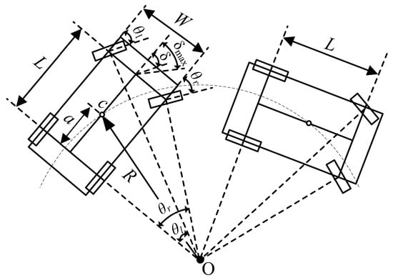
Figure 1.
Inspection robot steering model.
As shown in Figure 1, O is the steering center, c is the mass center of a vehicle, a is the distance from the mass center to the rear wheels, L is the distance between the front and rear wheels, W represents the distance between the front wheels, θl and θr are the steering angles of the left and right front wheels, respectively, δ is the Ackermann steering angle, δmax is the maximum steering angle of the Ackermann mechanism, and R is the turning radius. During the robot’s movement, the equation of its motion is expressed as Formula (1):
During the motion of the inspection robot, the Ackermann steering mechanism is subjected to the non-holonomic constraint, which is reflected in its limited Ackermann steering angle δ and turning radius R. The inspection robot with the Ackermann steering mechanism cannot have an arbitrary trajectory. Therefore, the planned path trajectory should meet the following conditions:
2.2. RRT* Algorithm
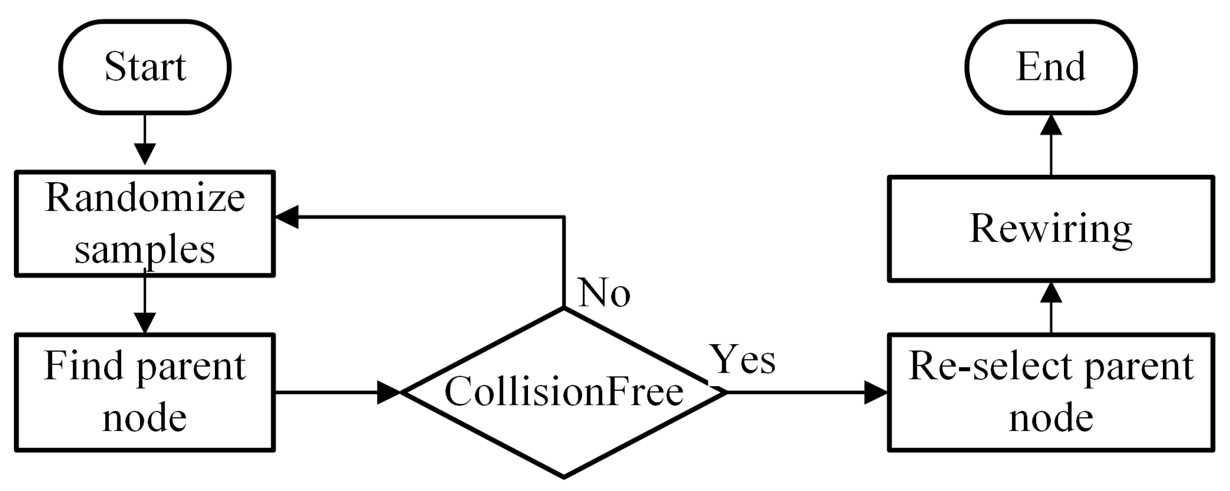
The RRT algorithm was first proposed by LaValle in 2001 [29]. It is a sampling-based path planning algorithm. The basic idea of RRT is to take the starting point as the root node and construct a tree covering the entire search space by randomly sampling nodes. When the tree touches the goal point, a unique path connecting the starting point and the goal point can be obtained, but the algorithm cannot guarantee that the path is optimal. The RRT* algorithm proposed by Karaman is an improved version of RRT, as it adds the steps of reselecting parent nodes and rewiring on the basis of the RRT [30]. These two processes complement each other, as reselecting the parent nodes minimizes the cost of the path, and rewiring reduces redundant nodes in the random tree. The pseudocode and flowchart of the RRT* algorithm are shown in Algorithm 1 and Figure 2, respectively, and the search process of the algorithm is shown in Figure 3.
| Algorithm 1: RRT* Algorithm |
| Input:N, Qinit, Qgoal |
| Result: A path from Qinit to Qgoal |
| T.init(); |
| for i = 1 to n do |
| Qrand ← Sample(N); |
| Qnear ← Nearest (Qrand, T); |
| Qnew ← Steer (Qrand, Qnear, StepSize); |
| Ei ← Edge (Qnew, Qnear); |
| If CollisionFree (N, Ei) then |
| T.addNode (Qnew) |
| Vnear ← Near (T, Qnew) |
| Qparent ← Chooseparent (Vnear, Qnear, Qnew) |
| T ← Rewire (T, Vnear, Qnew) |
| end if |
| end for |
| return T |

Figure 2.
Flowchart of RRT* algorithm.
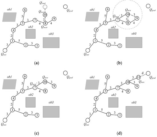
Figure 3.
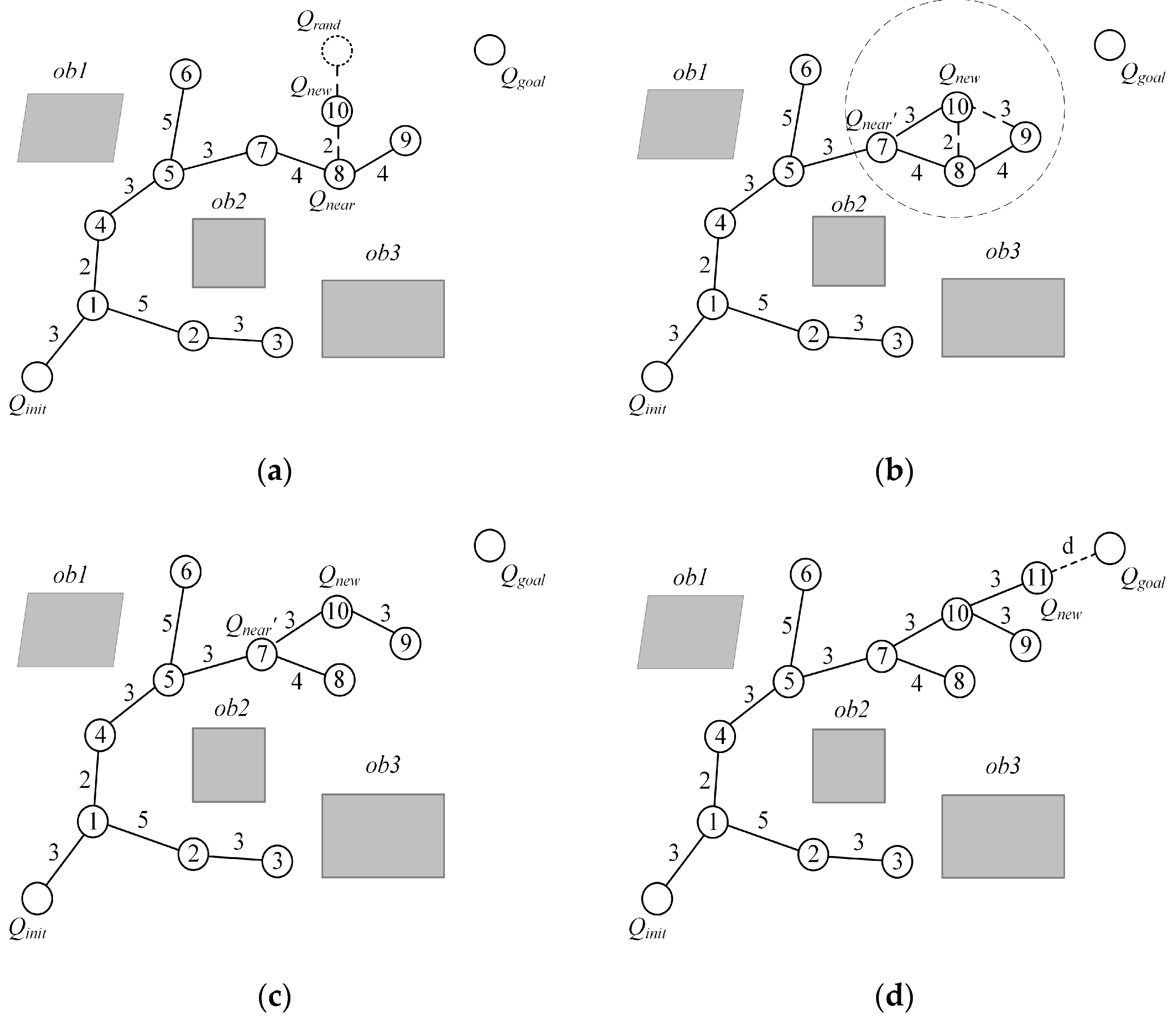
The search process of RRT*. (a) Find new node; (b) chooseparent; (c) rewiring; (d) find the target point.
The input of the RRT* algorithm includes the starting point Qinit, target point Qgoal, and environmental map N. The output is a path connecting the starting point to the target point. The RRT* initially generates a random sampling point Qrand and then it seeks out the nearest node Qnear within the random tree T relative to Qrand. The vector from Qnear to Qrand serves as the growth direction of the tree, along which a new node Qnew is produced with a preset step size. If there are no obstacles between Qnew and Qnear, the parent node of Qnew is designated as Qnear. (Figure 3a shows the above process). In Figure 3, in-circle numbers represent the sequentially generated nodes in the random tree, the numeric values on the connecting lines denote the path costs between two nodes, and gray blocks represent known obstacles in the environment.
After acquiring Qnew, all known nodes in the circle centered on Qnew and with a preset value ri as the radius are considered as candidate nodes, and the path cost required from Qnew to the start point Qinit via each candidate node is calculated sequentially. ri is defined by the Near function, as shown in Formula (3):
where η is a predefined radius, n is the number of current nodes, ζd is the volume of the circle with radius ri, d is the spatial dimension, and γ is an adjustable parameter used to adjust the search range. Subsequently, the candidate node corresponding to the lowest path cost is selected as the new parent node for Qnew. The chooseparent procedure is presented in Algorithm 2 and Figure 3b shows that the path from Qnew to Qinit though node 7 follows the sequence 10–7–5–4–1, with a corresponding cost of 11, the path from Qnew to Qinit though node 8 is 10–8–7–5–4–1, with a cost of 12, and the path from Qnew to Qinit through node 9 is 10–9–8–7–5–4–1, with a cost of 19. Consequently, node 7 is deemed the new parent node Qnear′ of Qnew.
| Algorithm 2: Chooseparent () |
| Input: Vnear, Qnear, Qnew Output: Qparent Qparent ← Qnear; cmin ← Cost (Qnear) + Distance (Qnew,Qnear); for each Qi in Vnear do c ← Cost (Qi) + Distance (Qnew,Qi); If c < cmin && CollisionFree (Qnew,Qi) then Qparent ← Qi; cmin ← c; end for return Qparent |
Finally, the rewiring operation is carried out, specifically to calculate the path cost of each candidate node to reach Qinit through Qnew. If the calculated path cost is smaller than the existing path cost, the algorithm abandons the original parent node and instead establishes a direct connection between Qnew and the candidate node. Figure 3b shows that the path for node 9 to reach Qinit through Qnew is 9–10–7–5–4–1, with a cost of 14. Originally, it is 9–8–7–5–4–1 with a cost of 16. Therefore, the connection of 9–8 is deleted and 9–10 is connected. (The rewiring results are shown in Figure 3c). The rewire procedure is presented in Algorithm 3.
| Algorithm 3: Rewire () |
| Input: Qi, Vnear, Qnew Output: T for each Qi in Vnear do If Cost (Qi) > Cost (Qnew) + Distance (Qnew,Qi) then If CollisionFree (Qnew,Qi) then Qparent ← Parent(Qi); T← Reconnect (Qnew,Qi); end if end if end for return T |
The RRT* algorithm continuously generates sample points and repeats the above steps. When the distance from the most recently generated new node Qnew to the target point Qgoal is less than the step size, the new node is directly connected to the target point, as shown in Figure 3d. In this way, the RRT* algorithm plans a collision-free path connecting the starting point to the goal point.
The RRT* algorithm has been widely used in various autonomous navigation machines due to its simple structure and fast search speed. However, in the environment of solar power plants, the RRT* algorithm faces the following challenges:
- (1)
- The conventional RRT* algorithm expands the growth of the tree by randomly generating sampling points. This step makes the random tree grow blindly, resulting in its inability to search for the target quickly. In other words, it has poor goal orientation;
- (2)
- In intricate environments such as narrow channels with limited passable areas, the RRT* algorithm requires more iterations to generate effective nodes to plan the path, which leads to a significant reduction in searching efficiency;
- (3)
- The path planned by RRT* consists of a series of discrete nodes and has a large number of turning points, and direct application can lead to unnecessary jerks and oscillations, affecting motion stability. Therefore, it is necessary to further optimize the path.
3. Improved RRT* Algorithm
In this section, an improved RRT* algorithm based on an adaptive target bias and heuristic circular sampling for the continuous narrow channels of solar power plants is proposed, which enhances the random tree’s ability to expand towards the target and substantially improves its search efficiency in narrow channels. Figure 4 illustrates the flowchart depicting the improved RRT* algorithm, and Algorithm 4 shows the pseudocode for the improved RRT*.
| Algorithm 4: Improved RRT* |
| Input: N, Qinit, Qgoal |
| Result: A path from Qinit to Qgoal |
| T.init(); |
| for i = 1 to n do |
| Qrand ← Adaptive Target Bias (Qgoal, λ, N); |
| Qnear ← Nearest (Qrand, T); |
| Qnew ← Steer (Qrand, Qnear, StepSize); |
| Ei ← Edge (Qnew, Qnear); If CollisionFree (N, Ei) is False: Qnew ← Heuristic Circular Sampling (Qnew, Qnear, δ); end if |
| If CollisionFree (Qnew, Qnear) then |
| T.addNode (Qnew) |
| Vnear ← Near (T, Qnew) |
| Qparent ← Chooseparent (Vnear, Qnear, Qnew) |
| T ← Rewire (T, Vnear, Qnew) If |Qnew − Qgoal|< Stepsize then T ← Path Prunning (T); T ← B-spine smoothing (T); |
|
end if end if |
| end for |
| returnT |
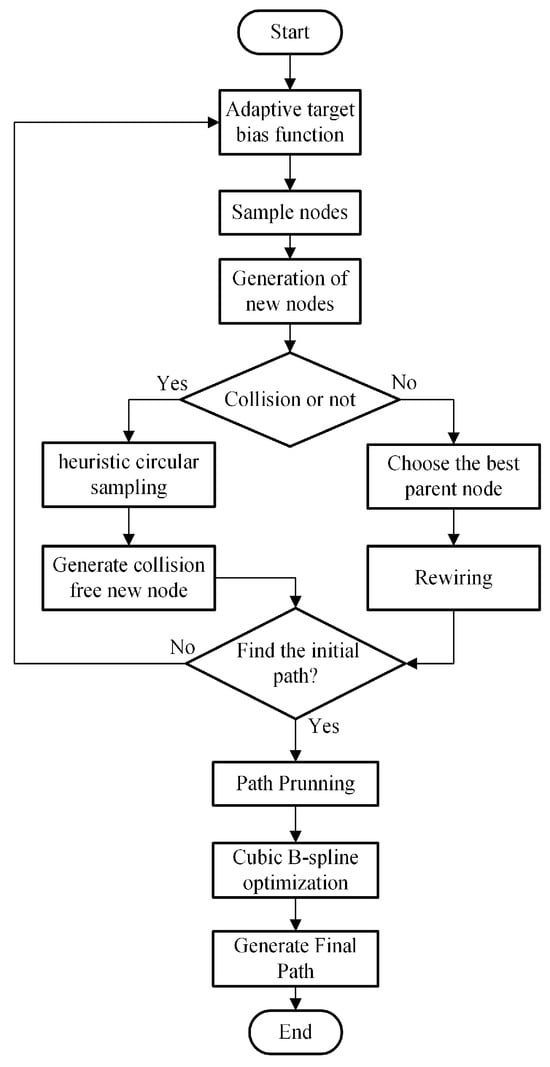
Figure 4.
The flowchart of improved RRT*.
Specifically, the algorithm introduces an adaptive target bias function prior to the random sampling step, and continuously adjusts the weight ratio between the target point and the random point during the planning process to accelerate the search speed. Subsequently, when the generated new node falls on obstacles flanking both sides of the narrow channel, a heuristic circular sampling strategy is adopted. This strategy significantly increases the probability of sampling points landing within the narrow channel, and elevates the algorithm’s search efficiency and stability. Furthermore, the path is pruned based on the minimum turning radius of the inspection robot, and a cubic B-spline curve is applied to optimize the path, enabling the inspection robot to operate smoothly and safely.
3.1. Adaptive Target Bias Strategy
In an effort to address the issues of slow search speed and protracted planning time caused by random sampling in the classic RRT* algorithm, this section proposes the adaptive target bias strategy method, for which the mathematical expression is presented in Formula (4):
where Qrand and Qgoal are the coordinates of the random sampling point and the target point, respectively; λ is a weight coefficient with a value of (0, 1). The main idea of the target bias strategy is to determine the generation of random points by adjusting the weight coefficients of Qrand and Qgoal. The value of λ influences the algorithm’s search and target bias capabilities. The smaller λ is, the closer the sampling point is to the region where Qrand is located, and the stronger the search ability is. On the contrary, the larger λ is, the closer the sampling point is to the region where Qgoal is located, and the stronger the target bias ability is. To further enhance the search efficiency of the algorithm, an adaptive weight adjustment is adopted, as elucidated in Formula (5):
where t represents the coefficient of change, which is determined by the distance between the new node and the target point, as well as the distance from the starting point to the target point. Simultaneously, we set the distance parameter n to ensure the rationality of weight λ under different environmental maps. When Qnew is situated further away from Qgoal, the sampling strategy focuses on searching the region; when Qnew is in proximity to Qgoal, the sampling strategy emphasizes the ability to bias the target. In essence, the adaptive target bias strategy motivates the random tree to search in areas far from the target point and lends bias towards the target in areas close to the target point, which allows for a significant improvement in search efficiency.
3.2. Heuristic Circular Sampling
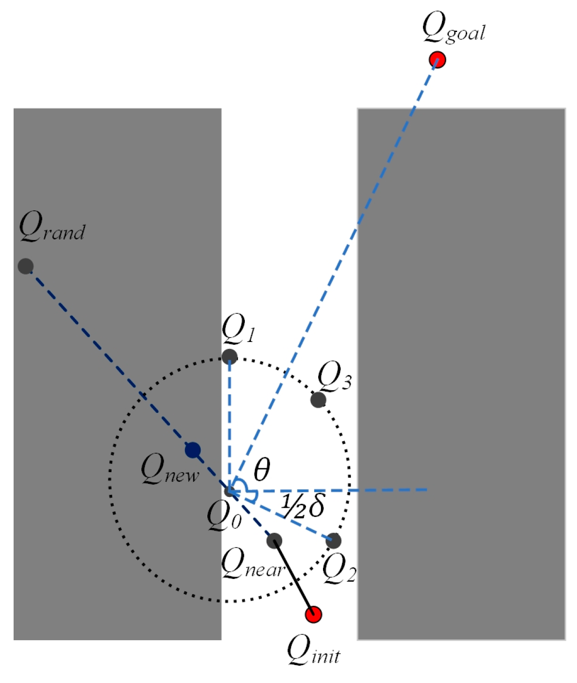
In an environment of continuous narrow channels where the passable area occupies a relatively small space, the nodes sampled by the conventional RRT* algorithm are prone to be generated within the obstacles, which leads to a reduction in the search efficiency. To solve this problem, this section adopts heuristic circular sampling combined with directional bias, and the sampling process in a narrow channel is shown in Figure 5.
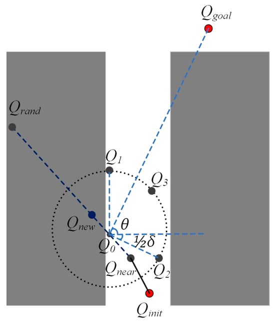
Figure 5.
Sampling process in the narrow channel.
When Qnew falls on the obstacles, the algorithm first computes the angle θ between the line connecting Q0 and Qgoal and the horizontal direction, and a predetermined directional deviation angle δ is introduced. Following this, a resampling procedure is undertaken on the circular arc which is centered at the midpoint Q0 of the line connecting Qnew and Qnear, with twice the step size of the radius and the center angle of θ + δ. Assuming that the coordinates of Q0 are (x0, y0), and the coordinates of the resample point Q3 are (x3, y3), the relationship can be expressed as follows:
As expressed in Formula (6), the horizontal angle θ, in conjunction with the directional deviation angle δ, collaboratively influences the generation of resampling points. This coordinated adjustment is designed to increase the probability of sampling nodes falling in narrow channels, and enhances the utilization rate of the nodes and the search efficiency.
3.3. Path Optimization
The path planned by the RRT* algorithm is composed of a sequence of discrete nodes lacking continuity and possessing numerous turning points, which can lead to unnecessary sharp turns and oscillations during the operation of the inspection robot. To improve the stability of its movement, further optimization of the path is necessary. In this section, path nodes are pruned based on the minimum turning radius of the inspection robot and the cubic B-spline curve is used to smooth the path. These processes ensure that the inspection robot can safely and seamlessly reach its destination point.
- (1)
- Path pruning based on minimum turning radius
Nodes on the path that fail to meet the constraint of the robot’s turning radius are pruned, the specific steps for which are as follows:
Step 1: Traverse all nodes in the path except for the starting and target points, and find the two adjacent nodes for each node;
Step 2: Calculate the angle between adjacent path segments in sequence and the path radius corresponding to this angle. If the radius is less than the minimum turning radius of the robot, it indicates that the path point cannot satisfy the robot’s turning and needs to be deleted;
Step 3: Repeat Step 2 until all path points meet the constraint conditions of the turning radius.
Path pruning is shown in Figure 6, in which Qi, Qi+1, and Qi+2 are three adjacent nodes with the corresponding path radius r. Due to the constraint of the turning radius, r must be bigger than the minimum turning radius Rmin of the inspection robot, as shown in Formula (7):
where α is the angle between vector and vector . If r is indeed smaller, the node Qi+1 is removed, and a direct connection is established between Qi and Qi+2. This pruning operation is repeated iteratively, ensuring that all the path points conform to the turning radius constraints.
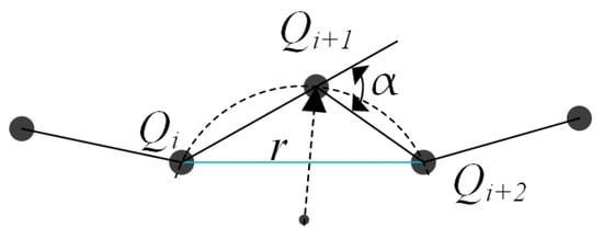
Figure 6.
Path pruning diagram.
- (2)
- B-spine Smoothing
In the pruned path, there still exist a number of tortuous nodes and discontinuous curvature. In order to ensure the continuous motion of inspection robots, the B-spline curve is adopted to fit the path points. Compared to the Bezier curve, the B-spline curve has characteristics such as high smoothness and local adjustability. The expression for the B-spline curve is shown in Formula (8):
where B(u) represents the B-spline curve; Bi,k(u) is the ith and kth B-spline basis function and Pi is the ith control point. To obtain a smoothed trajectory, the path nodes Qi are considered as control points Pi of the B-spline curve. The B-spline basis function is determined by a sequence of node vectors, which can be recursively derived by the Cox–deBoor algorithm:
where ui is the ith node, Bi,k(u) is the kth polynomial corresponding to the interval [ui, ui+1]. In the equation, if a kth B-spline basis function Bi,k(u) has n + 1 control points Pi, the required number of nodes is m + 1, which must satisfy Formula (11):
For a cubic B-spline curve, a set of non-decreasing sequences of node vectors is defined as [u0, u1..., un..., un+k], and u [0, 1]. To make the curve pass through the starting and target points of the path, the nodes at both ends have k repetitions, and we set:
Fitting the pruned path nodes by using cubic B-spline curves can significantly reduce the number of turning points and ameliorate the discontinuity in the path curvature. This improvement, in turn, enhances the overall stability of the autonomous operations of the inspection robot.
4. Simulation Results
To evaluate the performance of the improved RRT* algorithm, comparative experiments were conducted between the improved RRT*, RRT*, and informed RRT* in the simulation environments shown in Figure 7. Map 1, Map 2, and Map 3 had sizes of 100 m × 100 m, the step sizes of the the algorithms were 3, the distance parameter n was assigned a value of 2, and the directional deviation angle δ ranged from (−π/2) to (π/2). The simulation process was developed with Python 3.9 and related libraries such as Matplotlib 3.4.3, NumPy 1.20.3, and spicy 1.7.1. Matplotlib and NumPy were utilized to create the simulation environment and generate the path trajectory diagrams, while spicy was used to create the formulas. Operating environment: we used the Windows 10 system, the processor was an AMD Ryzen 7 5800 H, and the memory was 16 GB.
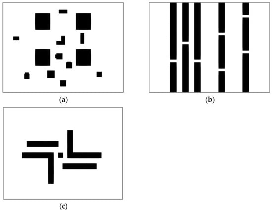
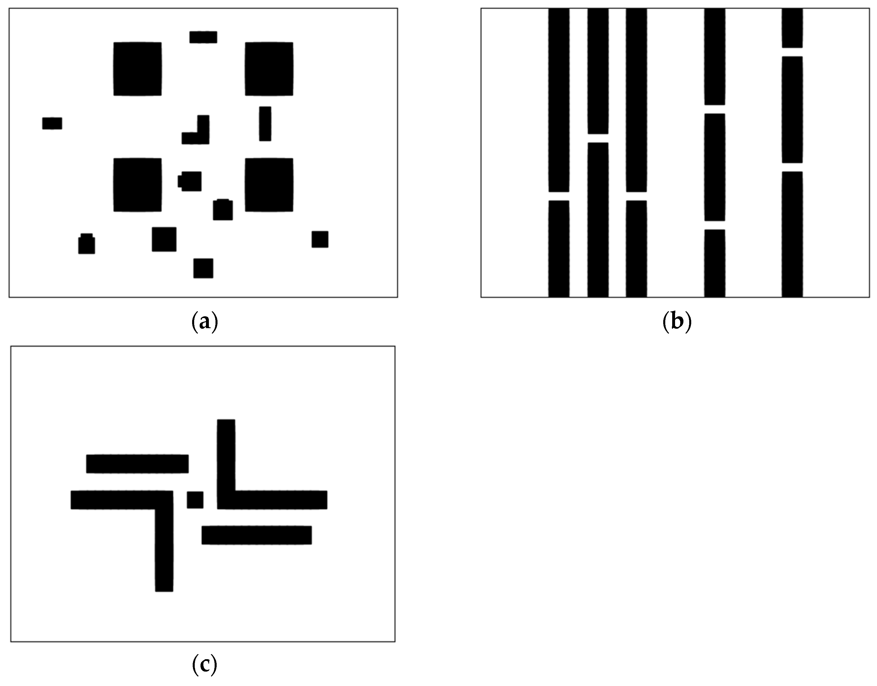
Figure 7.
Simulation environments. (a) Map 1; (b) Map 2; (c) Map 3.
4.1. Map 1
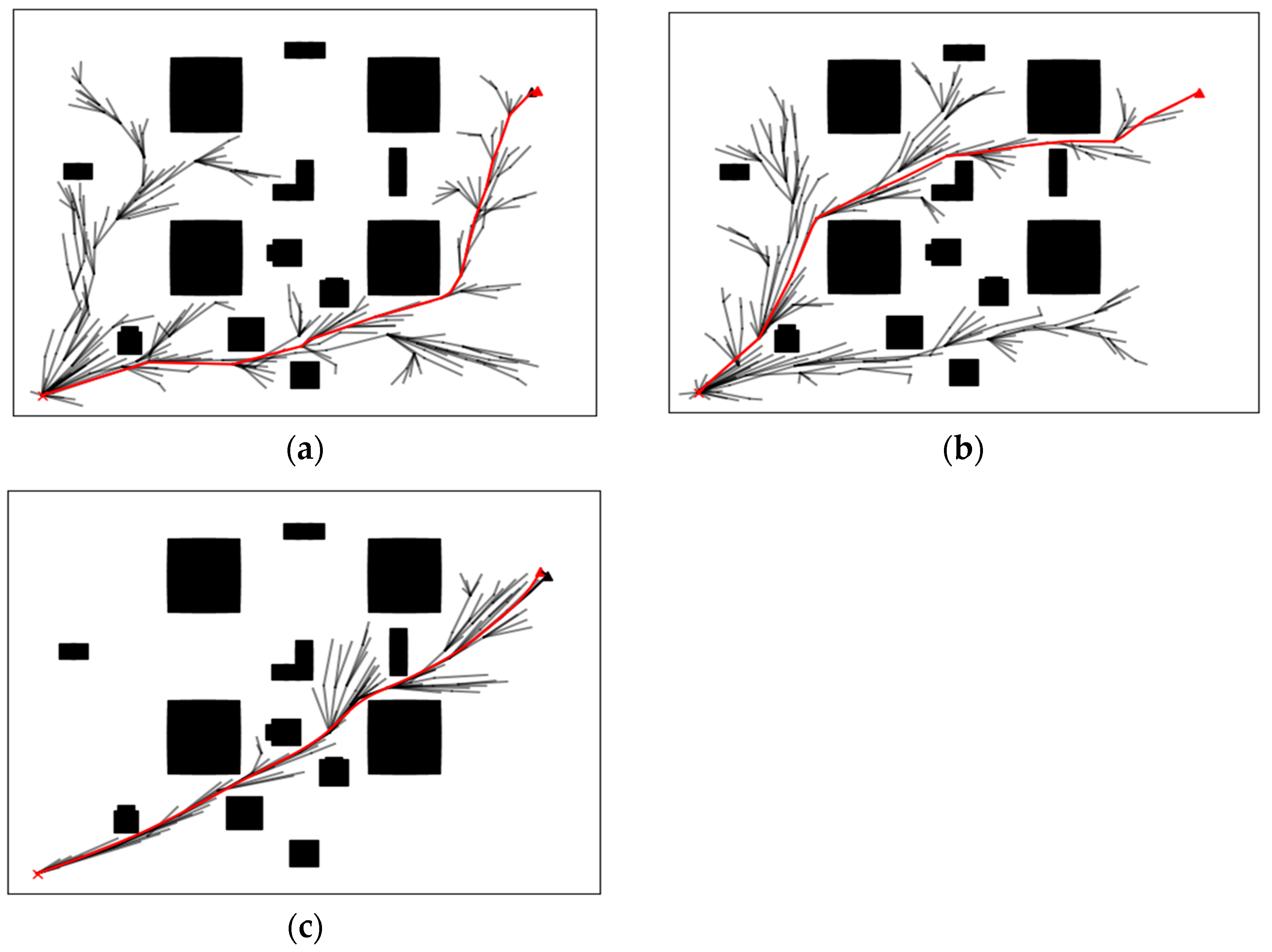
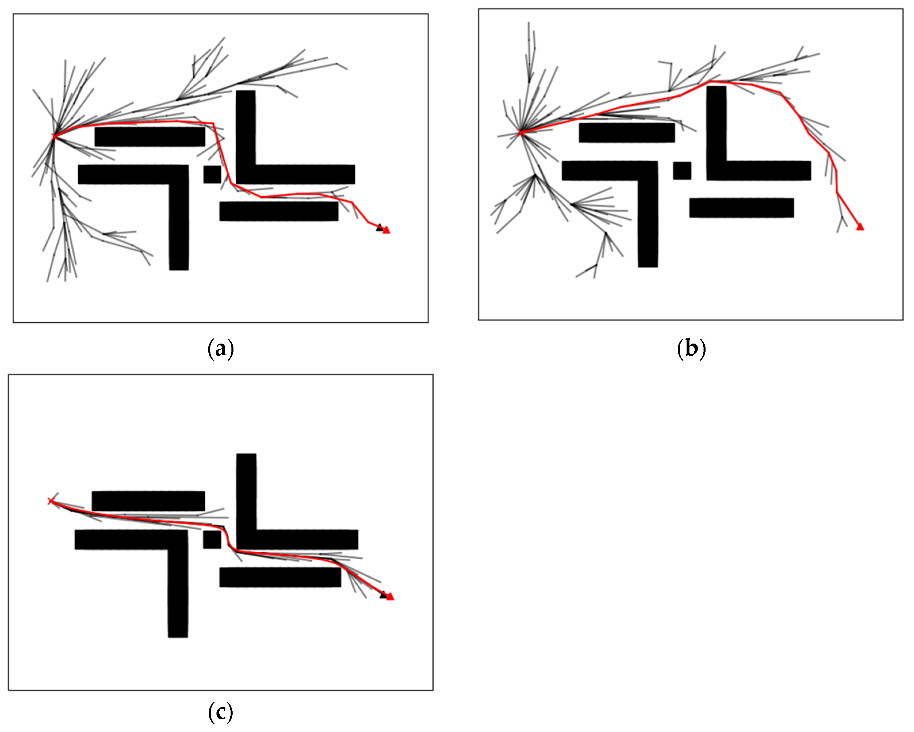
Figure 7a is a complex environment with multiple obstacles, and was used to validate the effectiveness of the improved algorithm in handling intricate environments. The coordinates of the starting point were (5, 5) and the coordinates of the target point were (90, 80), a total of 50 simulation experiments were conducted, and the representative results from the 50 simulations are represented by the red lines in Figure 8.
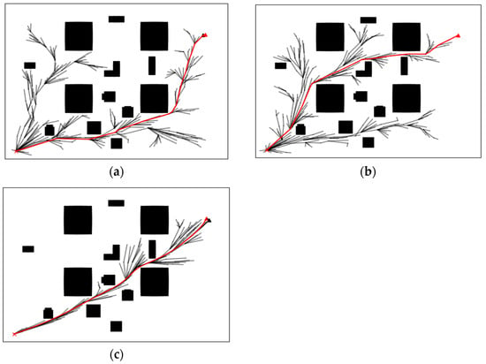
Figure 8.
Performance of the three algorithms in Map 1. (a) RRT*; (b) informed RRT*; (c) improved RRT*.
As can be seen from Figure 8, in the multi-obstacle environment, RRT* and informed RRT* enacted the spreading of random trees in multiple directions due to random samplings (the black line segments in the figure are the branching portions of the random trees). Additionally, these algorithms generated a number of turning nodes. However, the improved RRT* algorithm exhibited distinctive characteristics during the search process: its random tree gradually grew closer to the target point and generated efficient nodes even in regions with dense obstacles, which enhanced both the efficiency and quality of the path. At the same time, there are no obvious turning points on the planned path.
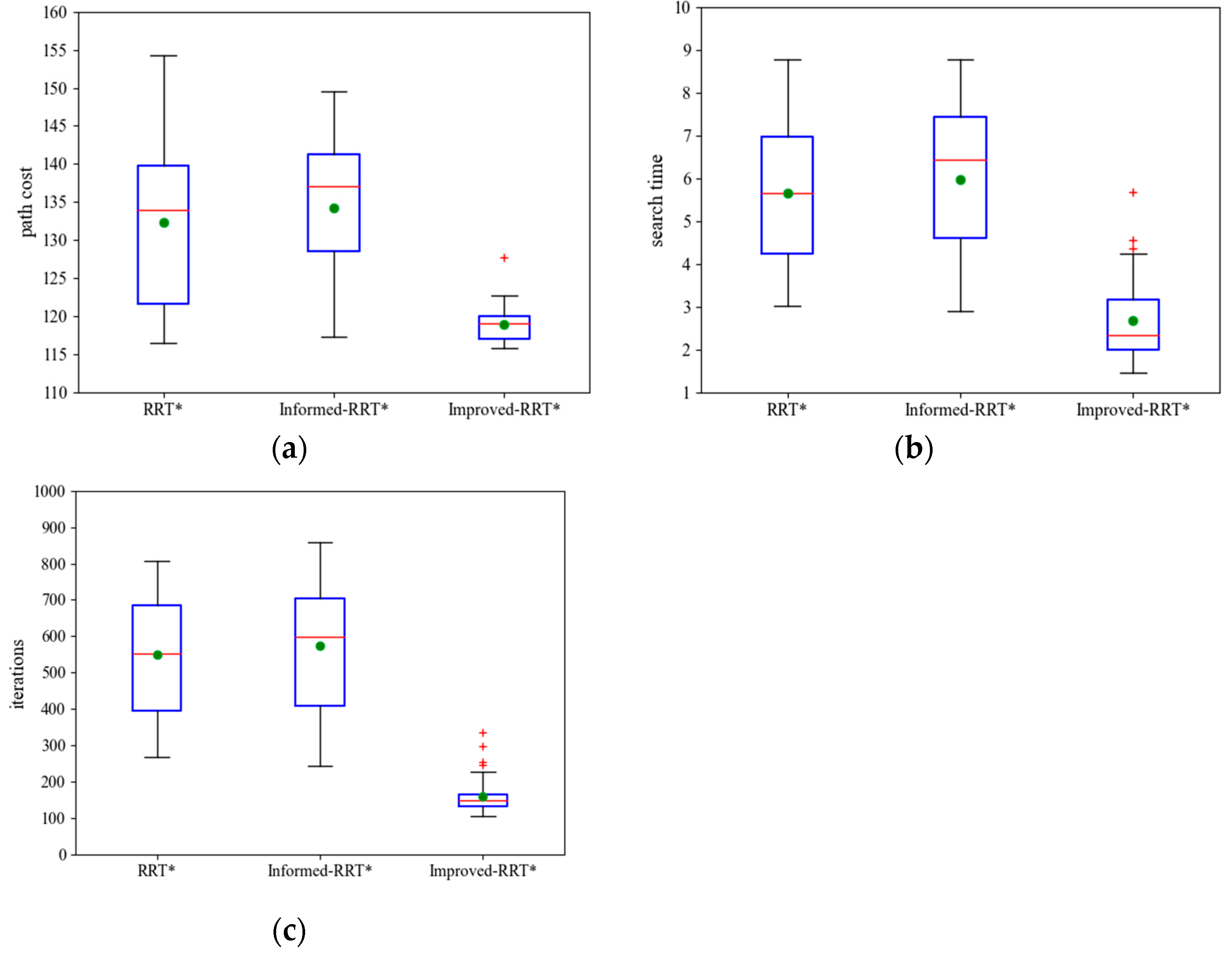
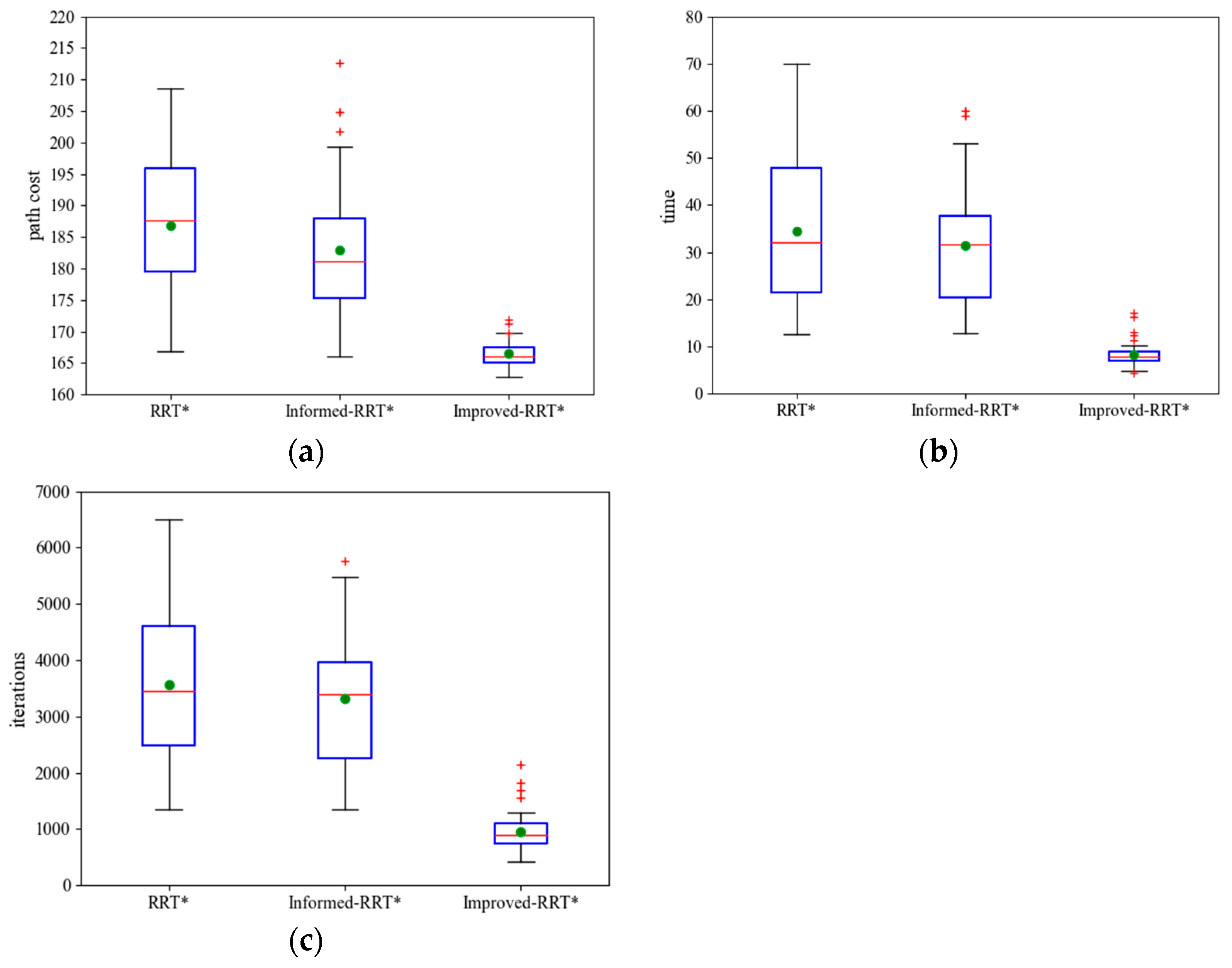
The data for 50 simulations of all three algorithms were organized into boxplots, as shown in Figure 9, and the statistical data of the boxplots are shown in Table 1. The red line, green bullet, and red crosses in Figure 9 represent the median, mean, and outliers of a set of data, respectively. Boxplots can well reflect the characteristics of the distribution of raw data. The smaller the box size of the boxplot, the more concentrated the distribution of a set of data is. To visually compare the path planning of the three algorithms, the statistics include the average path cost, average search time, and average number of iterations. These metrics, as a general case of a set of data, reflect well the performance of the algorithms. From Figure 9, it can be seen that the improved RRT* algorithm outperformed both the RRT* algorithm and the informed RRT* algorithm in these aspects. It had a shorter path length, reduced search time, and fewer iterations. Moreover, the distribution of the box lines in the improved RRT* algorithm’s boxplots was more concentrated compared with RRT* and informed RRT*, which indicated that there was a small difference in the results of each path planning of the improved algorithm. However, it is worth noting that there were a few outliers in the boxplots of the improved algorithm and these outliers result from the inherent randomness of the algorithm itself. It can be seen from Table 1 that, compared with the RRT* algorithm and informed RRT* algorithm, improved RRT* reduced the average path cost by 10.16% and 11.39%, the average search time by 52.65% and 55.18%, and the number of iterations by 70.78% and 72.91%, respectively. The outcome indicated that the improved algorithm effectively enhanced the search efficiency and stability.
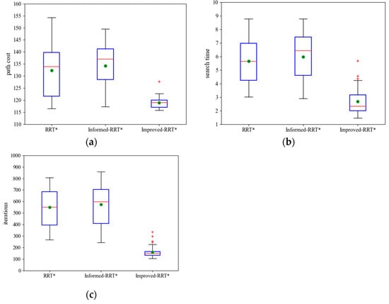
Figure 9.
Map 1 simulation boxplots. (a) Path cost; (b) search time; (c) iterations.

Table 1.
Map 1 simulation data.
4.2. Map 2
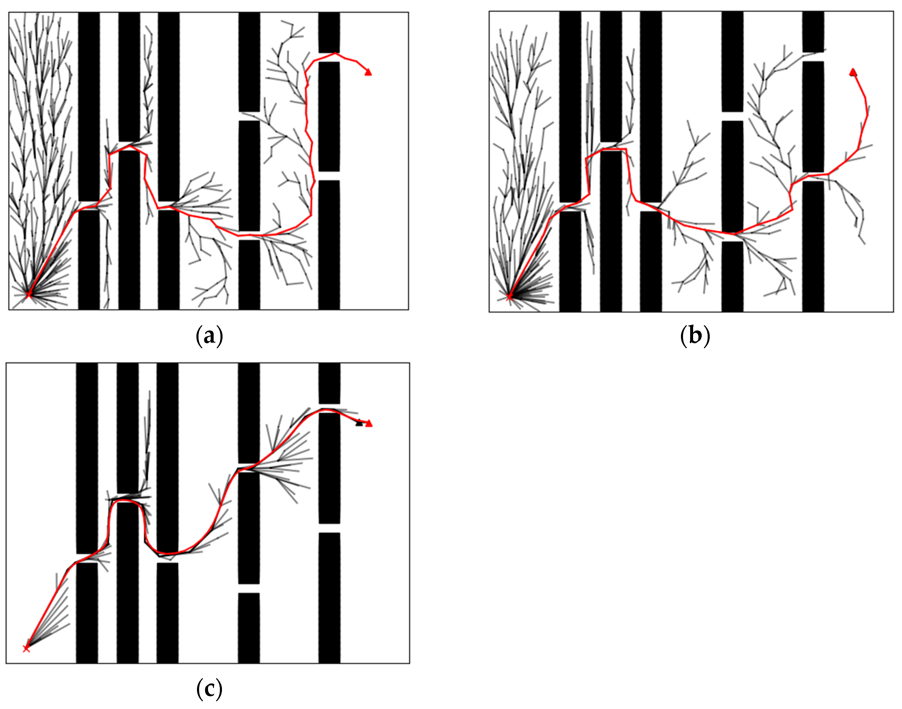
In order to verify the effectiveness of the improved algorithm in the narrow and long channel shown in Map 2, the coordinates of the starting point location were set to (5, 5) and the coordinates of the target point location were set to (90, 80). The simulation results are shown in Figure 10. From Figure 10, it can be seen that, in the narrow and long channel, the random trees of the RRT* algorithm and the informed RRT* algorithm both grew densely near the region of the starting point and sparsely near the region of the target point. In addition, a number of redundant nodes were generated in the narrow space, which led to a significant reduction in the searching efficiency and poor quality of paths. The improved algorithm’s random tree grew more towards the target point and generated fewer redundant nodes, while the planned path quality was higher. The data on the path cost, search time, and iterations for 50 simulations of all three of the algorithms were organized into boxplots, as shown in Figure 11. Moreover, Table 2 provides the average values derived from the collected data.
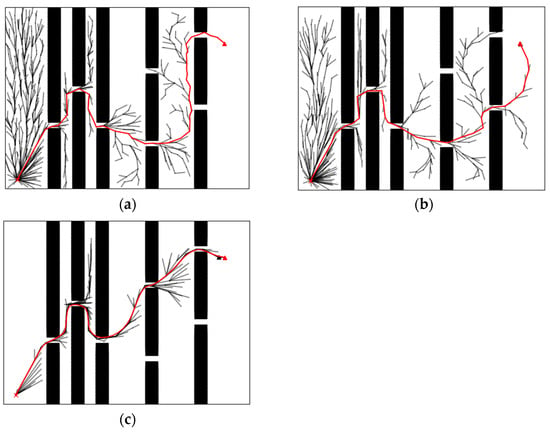
Figure 10.
Performance of the three algorithms in Map 2. (a) RRT*; (b) informed RRT*; (c) improved RRT*.
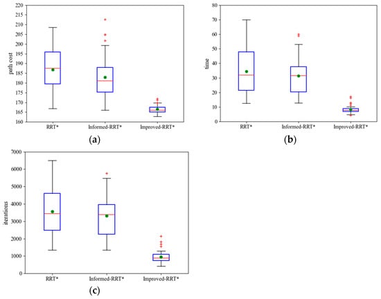
Figure 11.
Map 2 simulation boxplots. (a) Path cost; (b) search time; (c) iterations.
Table 2.
Map 2 simulation data.
By analyzing Figure 11 and Table 2, it can be seen that the improved RRT* algorithm reduced the average path cost by 10.93% and 8.99%, the average search time by 76.1% and 73.87%, and the number of iterations by 73.41% and 71.5%, respectively, in the environment of Map 2. The result shows that the improved RRT* algorithm effectively enhanced the search efficiency and stability of the RRT* algorithm.
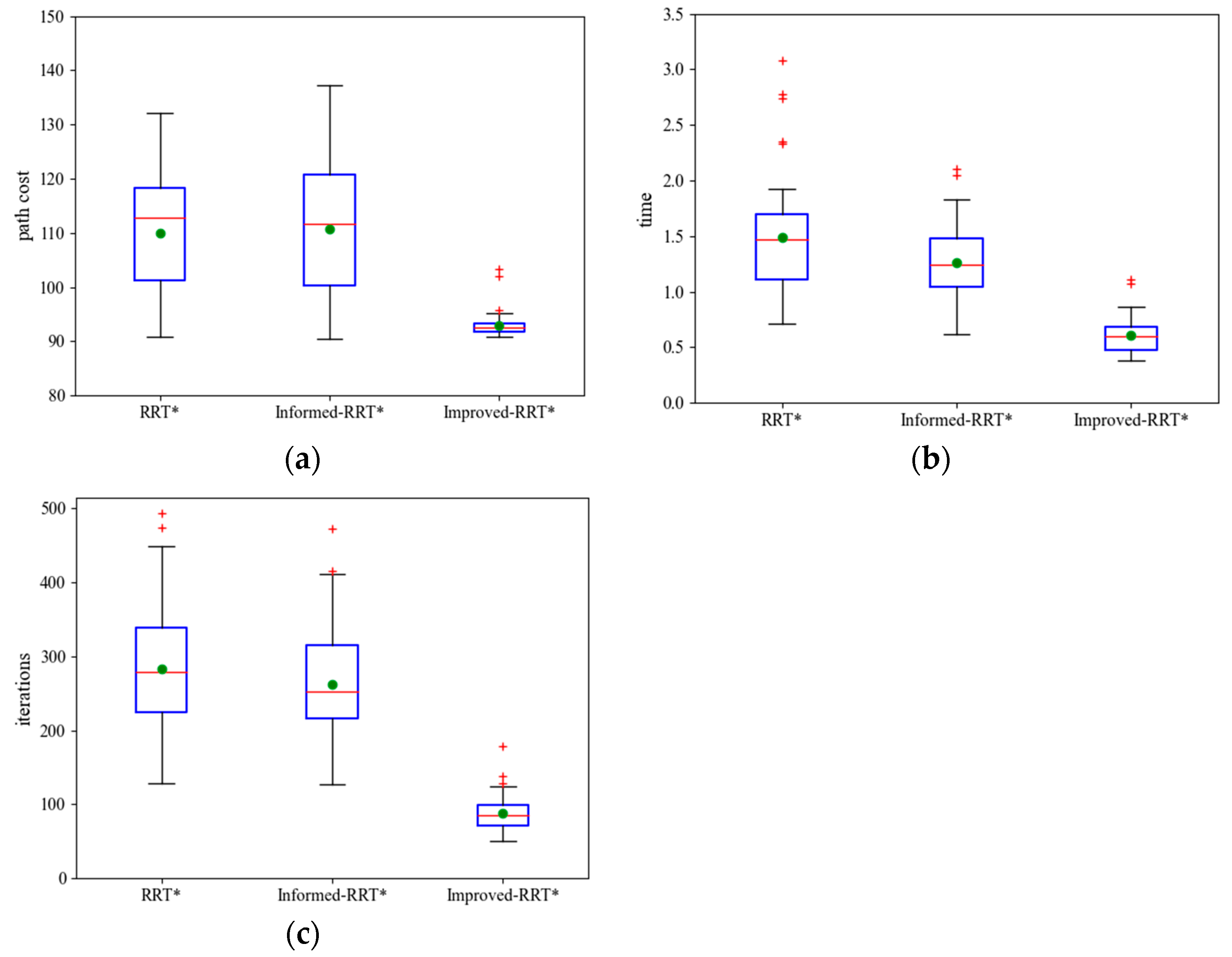
4.3. Map 3
Map 3 is shown in Figure 7c. The start coordinates were set to (10, 60) and the goal coordinates were set to (90, 30). Figure 12 shows the performance of the three algorithms. From the simulation results, we can see that the random trees of RRT* and informed RRT* both have instances of bypassing narrow channels when searching for the target point, which is due to their inability to generate effective nodes in narrow channels. On the contrary, the improved algorithm can reach the target point through narrow channels. Figure 13 shows the data on the path cost, search time, and iterations for 50 simulations of all three algorithms and Table 3 provides the average values derived from the collected data. In Figure 13, the evaluation indexes show that the improved algorithm outperforms the other two algorithms in terms of search efficiency. Meanwhile, the statistics in Table 3 show that the improved algorithm has better stability.
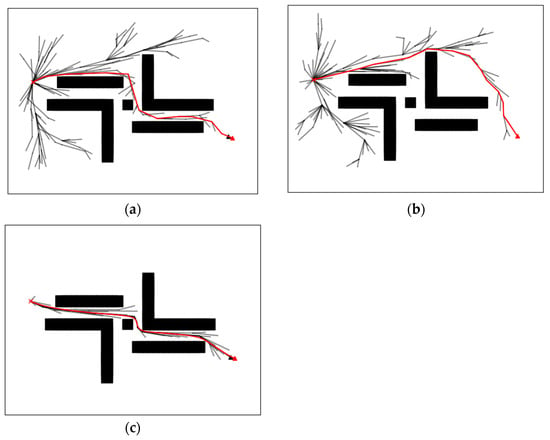
Figure 12.
Performance of the three algorithms in Map 3. (a) RRT*; (b) informed RRT*; (c) improved RRT*.
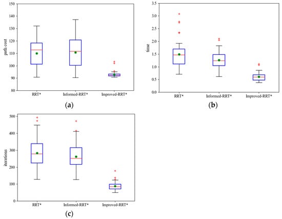
Figure 13.
Map 3 simulation boxplots. (a) Path cost; (b) search time; (c) iterations.
Table 3.
Map 3 simulation data.
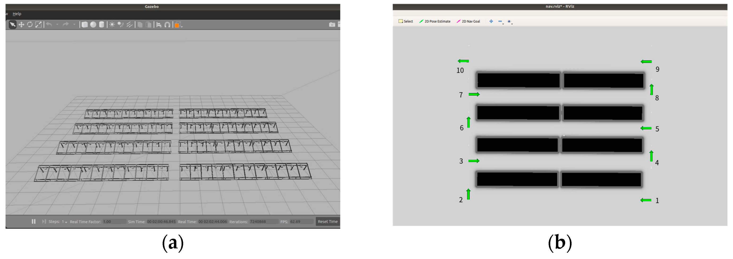
4.4. Solar Power Station Environment
To verify the applicability of the proposed RRT* algorithm to the actual work of inspection robots, a simulation comparison was conducted between the improved RRT* algorithm and the RRT* algorithm in the ROS system. Initially, multiple rows of PV panels were constructed in the ROS Gazebo simulation, as depicted in Figure 14a. Each row of PV panels measured 7 m in length and 1 m in width, and had a horizontal spacing of 2 m. To avoid the inspection robot colliding with the PV panels during its driving, the area containing the PV panels was inflated. Simultaneously, a multi-objective navigation strategy was adopted for the inspection robot to achieve full coverage of the PV panels. A two-dimensional environment map and the setting and orientation of each target point are illustrated in Figure 14b, and the inspection robot started from point 1 and passed through the PV panels in order of numbering to traverse all of them.
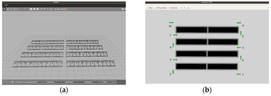
Figure 14.
Solar power station environment. (a) Gazebo environment; (b) rviz environment.
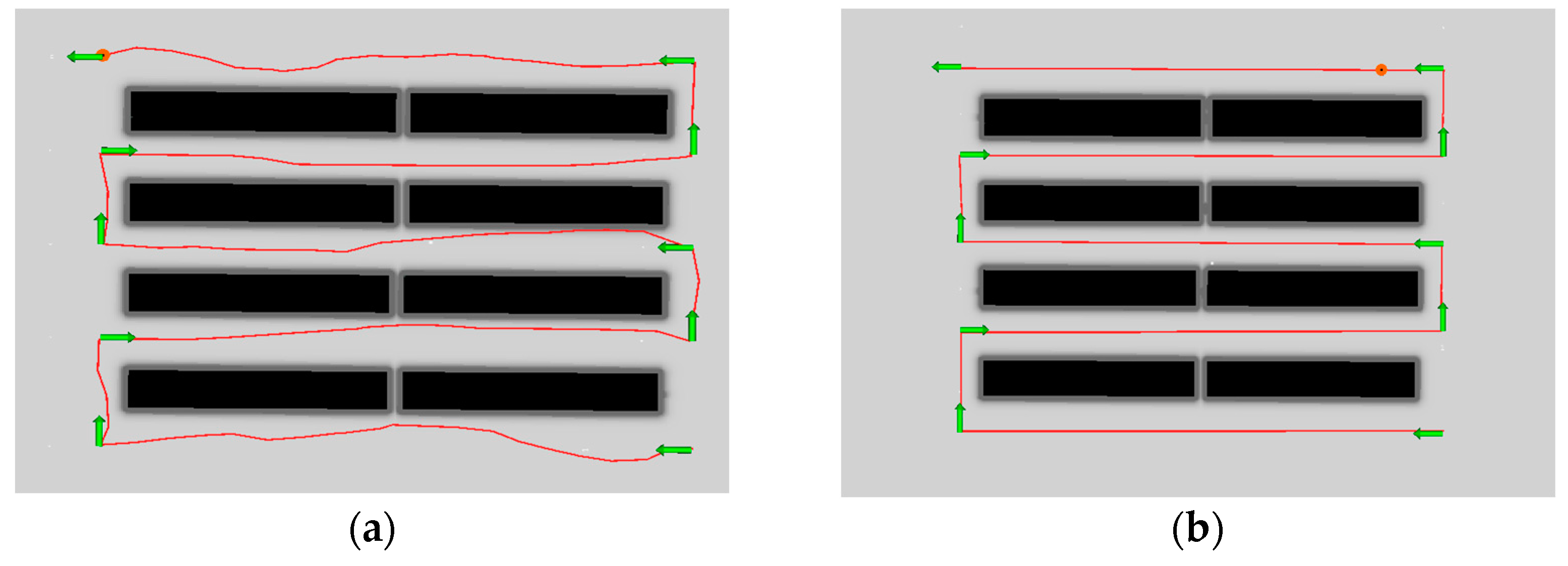
Simulation experiments on RRT* and improved RRT* were conducted in the two-dimensional environmental map of the PV plant, and the results and data are illustrated in Figure 15 and Table 4. From Figure 15, it can be seen that the path planned by the RRT* algorithm exhibited numerous turning points in the solar power plants environment, which affected the detection efficiency and safety of the inspection robot. In contrast, the path planned by the algorithm formulated in this paper had no obvious tortuous points in narrow and long channels, making it more suitable for the driving requirements of the inspection robot.

Figure 15.
Performance of the two algorithms in the solar power station. (a) RRT*, (b) improved RRT*.
Table 4.
Solar power station simulation data.
As can be seen from Table 4, the improved algorithm reduced the search time, path cost, and number of iterations by 62.06%, 1.6%, and 45.17%, respectively, compared to the RRT * algorithm.
Based on the above simulation experiments, it can be concluded that the improved-RRT* algorithm presented in this paper effectively enhances the search efficiency, path quality, and overall stability of the RRT* algorithm in the narrow channel environment of the solar power plant.
4.5. Discussion
In this study, we proposed an improved RRT* algorithm which aimed to improve the operational efficiency and safety of inspection robots for solar power plants. The traditional RRT* algorithm has a simple structure and strong adaptability, but its search efficiency and stability are low in complex environments. At the same time, the planned path tends to have a large number of turning nodes and is not smooth enough. The algorithm proposed in this paper introduced an adaptive target bias function, heuristic circular sampling combined with a direction deviation strategy, path pruning based on minimum turning radius, and path smoothing based on the cubic B-spline curve on the basis of the RRT* algorithm. These improvements accelerate the growth of random trees and improve the quality of planned paths. The improved algorithm was compared with the traditional RRT* algorithm through detailed simulation experiments. The result indicated that, compared with RRT*, the improved RRT* algorithm reduces the search time, number of iterations, and path cost by 62.06%, 45.17%, and 1.6%, respectively, in narrow channels of a solar power plant. Meanwhile, the improved algorithm has a higher search efficiency and stability, as well as a higher path quality, which can better meet the job requirements of inspection robots.
However, our research is limited to testing in simulated environments. In the future, verification is needed using actual robots to determine their performance in the real world. In addition, in some tasks that require real-time applications, the search time of the algorithm needs to be further reduced. Future research directions include broader performance evaluation, the automatic optimization of algorithm parameters, and integration with other path planning methods.
5. Conclusions
The RRT* algorithm is characterized by probabilistic completeness and asymptotic optimality, but it has problems such as a slow convergence speed and low search efficiency in narrow channels of solar power plants. To address these issues, this paper proposed an improved RRT* algorithm, including the adaptive target bias function, the heuristic circular sampling strategy, path pruning based on the minimum turning radius, and path optimization based on the B-spine curve. The experiments and analyses conducted in this paper demonstrate that the proposed algorithm can effectively improve the search efficiency of RRT* in narrow channels of solar power plants. Moreover, the proposed algorithm exhibits higher stability.
However, the algorithm in this paper also has some limitations: (1) The parameters used in the proposed algorithm are not universally applicable to other environments. The need for adaptive parameterization is recognized as a focus for future research. (2) How to achieve real-time and efficient obstacle avoidance when dealing with moving objects will be the main content of our future research.
Author Contributions
Conceptualization, F.W. and D.Z.; methodology, Y.G., Z.C. and X.G.; software, Y.G.; validation, X.G. and W.C.; investigation, Y.G.; data curation, X.G.; writing—original draft preparation, Y.G.; writing—review and editing, Y.G., F.W. and Z.C. All authors have read and agreed to the published version of the manuscript.
Funding
This research was funded by Anhui Natural Science Foundation (2008085UD09); Anhui University Collaborative Innovation Project (GXXT-2021-010); Anhui Construction Plan Project (2022-YF016, 2022-YF065, 2023-YF050); Open Project of Anhui Simulation Design and Modern Manufacture Engineering Technology Research Center (SGCZXZD2101).
Institutional Review Board Statement
Not applicable.
Informed Consent Statement
Not applicable.
Data Availability Statement
Data sharing not applicable.
Acknowledgments
We would like to acknowledge the support from Anhui Natural Science Foundation, Anhui Provincial Department of Education, Anhui Provincial Department of Housing and Urban Rural Development.
Conflicts of Interest
The authors declare no conflict of interest.
References
- Zhao, Z.-Y.; Zhang, S.-Y.; Hubbard, B.; Yao, X. The emergence of the solar photovoltaic power industry in China. Renew. Sustain. Energy Rev. 2013, 21, 229–236. [Google Scholar] [CrossRef]
- Li, H.; Lin, H.; Tan, Q.; Wu, P.; Wang, C.; De, G.; Huang, L. Research on the policy route of China’s distributed photovoltaic power generation. Energy Rep. 2020, 6, 254–263. [Google Scholar] [CrossRef]
- Du, J.; Zheng, J.; Liang, Y.; Liao, Q.; Wang, B.; Sun, X.; Zhang, H.; Azaza, M.; Yan, J. A theory-guided deep-learning method for predicting power generation of multi-region photovoltaic plants. Eng. Appl. Artif. Intell. 2023, 118, 105647. [Google Scholar] [CrossRef]
- Huo, J.; Pan, B. Study the path planning of intelligent robots and the application of blockchain technology. Energy Rep. 2022, 8, 5235–5245. [Google Scholar] [CrossRef]
- Aslan, M.F.; Durdu, A.; Sabanci, K. Goal distance-based UAV path planning approach, path optimization and learning-based path estimation: GDRRT*, PSO-GDRRT* and BiLSTM-PSO-GDRRT*. Appl. Soft Comput. 2023, 137, 110156. [Google Scholar] [CrossRef]
- Zhang, L.; Zhang, Y.; Li, Y. Path planning for indoor Mobile robot based on deep learning. Optik 2020, 219, 165096. [Google Scholar] [CrossRef]
- Sizkouhi, A.M.; Esmailifar, S.; Aghaei, M.; Karimkhani, M. RoboPV: An integrated software package for autonomous aerial monitoring of large scale PV plants. Energy Convers. Manag. 2022, 254, 115217. [Google Scholar] [CrossRef]
- Ma, L.; Hartmann, T. A proposed ontology to support the hardware design of building inspection robot systems. Adv. Eng. Inform. 2023, 55, 101851. [Google Scholar] [CrossRef]
- Gasparetto, A.; Boscariol, P.; Lanzutti, A.; Vidoni, R. Path planning and trajectory planning algorithms: A general overview. In Motion and Operation Planning of Robotic Systems: Background and Practical Approaches; Springer: Cham, Switzerland, 2015; pp. 3–27. [Google Scholar]
- Hart, P.E.; Nilsson, N.J.; Raphael, B. A formal basis for the heuristic determination of minimum cost paths. IEEE Trans. Syst. Sci. Cybern. 1968, 4, 100–107, Erratum in ACM SIGART Bull. 1972, 28–29. [Google Scholar] [CrossRef]
- Khatib, O. Real-time obstacle avoidance for manipulators and mobile robots. Int. J. Robot. Res. 1986, 5, 90–98. [Google Scholar] [CrossRef]
- Huang, G.; Ma, Q. Research on path planning algorithm of autonomous vehicles based on improved RRT algorithm. Int. J. Intell. Transp. Syst. Res. 2022, 20, 170–180. [Google Scholar] [CrossRef]
- Li, C.; Huang, X.; Ding, J.; Song, K.; Lu, S. Global path planning based on a bidirectional alternating search A* algorithm for mobile robots. Comput. Ind. Eng. 2022, 168, 108123. [Google Scholar] [CrossRef]
- Li, Y.; Wei, W.; Gao, Y.; Wang, D.; Fan, Z. PQ-RRT*: An improved path planning algorithm for mobile robots. Expert Syst. Appl. 2020, 152, 113425. [Google Scholar] [CrossRef]
- Fan, J.; Chen, X.; Liang, X. UAV trajectory planning based on bi-directional APF-RRT* algorithm with goal-biased. Expert Syst. Appl. 2023, 213, 119137. [Google Scholar] [CrossRef]
- LaValle, S.M.; Kuffner, J.J., Jr. Randomized kinodynamic planning. Int. J. Robot. Res. 2001, 20, 378–400. [Google Scholar] [CrossRef]
- Wan, X.; Ye, Y.; Leitao, Y.; Zhu, L. A global path planning algorithm based on improved RRT*. Control Decis. 2022, 37, 829–838. [Google Scholar]
- Ma, G.; Duan, Y.; Li, M.; Xie, Z.; Zhu, J. A probability smoothing Bi-RRT path planning algorithm for indoor robot. Futur. Gener. Comput. Syst. 2023, 143, 349–360. [Google Scholar] [CrossRef]
- Liu, Y.; Li, C.; Yu, H.; Song, C. NT-ARS-RRT: A novel non-threshold adaptive region sampling RRT algorithm for path planning. J. King Saud Univ.—Comput. Inf. Sci. 2023, 35, 101753. [Google Scholar] [CrossRef]
- Karaman, S.; Frazzoli, E. Sampling-based algorithms for optimal motion planning. arXiv 2011, arXiv:1105.1186. [Google Scholar]
- Liao, B.; Wan, F.; Hua, Y.; Ma, R.; Zhu, S.; Qing, X. F-RRT*: An improved path planning algorithm with improved initial solution and convergence rate. Expert Syst. Appl. 2021, 184, 115457. [Google Scholar] [CrossRef]
- Yu, S.; Chen, J.; Liu, G.; Tong, X.; Sun, Y. SOF-RRT*: An improved path planning algorithm using spatial offset sampling. Eng. Appl. Artif. Intell. 2023, 126, 106875. [Google Scholar] [CrossRef]
- Nasir, J.; Islam, F.; Malik, U.; Ayaz, Y.; Hasan, O.; Khan, M.; Muhammad, M.S. RRT*-SMART: A rapid convergence implementation of RRT*. Int. J. Adv. Robot. Syst. 2013, 10, 299. [Google Scholar] [CrossRef]
- Adiyatov, O.; Varol, H.A. Rapidly-exploring random tree based memory efficient motion planning. In Proceedings of the 2013 IEEE International Conference on Mechatronics and Automation, Takamatsu, Japan, 4–7 August 2013; pp. 354–359. [Google Scholar]
- Gammell, J.D.; Srinivasa, S.S.; Barfoot, T.D. Informed RRT*: Optimal sampling-based path planning focused via direct sampling of an admissible ellipsoidal heuristic. In Proceedings of the 2014 IEEE/RSJ International Conference on Intelligent Robots and Systems, Chicago, IL, USA, 14–18 September 2014; pp. 2997–3004. [Google Scholar]
- Ding, J.; Zhou, Y.; Huang, X.; Song, K.; Lu, S.; Wang, L. An improved RRT* algorithm for robot path planning based on path expansion heuristic sampling. J. Comput. Sci. 2023, 67, 101937. [Google Scholar] [CrossRef]
- Liu, H.; Zhang, S.; Duan, Y.; Jia, W.; Shen, Y. Orchard Robot Motion Planning Algorithm Based on Improved Bidirectional RRT. Trans. Chin. Soc. Agric. Mach. 2022, 53, 31–39. [Google Scholar]
- Veneri, M.; Massaro, M. The effect of Ackermann steering on the performance of race cars. Veh. Syst. Dyn. 2021, 59, 907–927. [Google Scholar] [CrossRef]
- Shen, J.; Fu, X.; Wang, H.; Shen, S. Fast path planning for underwater robots by combining goal-biased Gaussian sampling with focused optimal search. Comput. Electr. Eng. 2021, 95, 107412. [Google Scholar] [CrossRef]
- Guo, J.; Xia, W.; Hu, X.; Ma, H. Feedback RRT* algorithm for UAV path planning in a hostile environment. Comput. Ind. Eng. 2022, 174, 108771. [Google Scholar] [CrossRef]


Disclaimer/Publisher’s Note: The statements, opinions and data contained in all publications are solely those of the individual author(s) and contributor(s) and not of MDPI and/or the editor(s). MDPI and/or the editor(s) disclaim responsibility for any injury to people or property resulting from any ideas, methods, instructions or products referred to in the content. |
© 2023 by the authors. Licensee MDPI, Basel, Switzerland. This article is an open access article distributed under the terms and conditions of the Creative Commons Attribution (CC BY) license (https://creativecommons.org/licenses/by/4.0/).