Abstract
Homography estimation for infrared and visible images is a critical and fundamental task in multimodal image processing. Recently, the coarse-to-fine strategy has been gradually applied to the homography estimation task and has proved to be effective. However, current coarse-to-fine homography estimation methods typically require the introduction of additional neural networks to acquire multi-scale feature maps and the design of complex homography matrix fusion strategies. In this paper, we propose a new unsupervised homography estimation method for infrared and visible images. First, we design a novel coarse-to-fine strategy. This strategy utilizes different stages in the regression network to obtain multi-scale feature maps, enabling the progressive refinement of the homography matrix. Second, we design a local correlation transformer (LCTrans), which aims to capture the intrinsic connections between local features more precisely, thus highlighting the features crucial for homography estimation. Finally, we design an average feature correlation loss (AFCL) to enhance the robustness of the model. Through extensive experiments, we validated the effectiveness of all the proposed components. Experimental results demonstrate that our method outperforms existing methods on synthetic benchmark datasets in both qualitative and quantitative comparisons.
1. Introduction
Due to the advancement of multi-sensor technology, multimodal images have received wide attention and applications in image processing. Homography estimation represents the projection transformation between two images, an essential technique for the fusion and alignment of multimodal images [1,2,3]. Although homography estimation methods are relatively mature under single image conditions, their complexity and challenges increase when dealing with infrared and visible images. Therefore, in-depth research on this specific scenario is critical, especially in application areas such as multi-sensor data fusion [4,5,6], environmental monitoring [7], disaster emergency response [8,9], scene classification [10], laser imaging [11], and 3D hand pose estimation [12].
Traditional methods typically employ extractors [13,14,15] to extract key points and descriptors from the image, followed by matching algorithms to obtain the corresponding points, and direct linear transform (DLT) [16] with outlier rejection [17,18,19] to estimate the homography matrix. This approach has been widely adopted in a single imaging modality, such as visible images, resulting in relatively established solutions. When dealing with scenes containing both infrared and visible images, however, traditional methods face challenges such as unstable feature extraction and reduced matching accuracy. This is because these two imaging modalities have different physical properties and visual characteristics, e.g., differences in spectral range and illumination conditions [20,21]. These problems constrain the effectiveness and accuracy of traditional methods in this particular scenario.
Traditional methods highly rely on the quality of feature points, whereas deep learning methods exhibit improved robustness and accuracy due to end-to-end automated feature learning. DeTone et al. [22] carried out a seminal study, introducing deep learning into homography estimation, using a VGG-like network architecture that outputs the displacement vectors of the four corners to compute the homography matrix further. In recent years, there have been numerous research efforts to optimize performance further, some focusing on coarse-to-fine strategies [23,24,25,26,27,28]. These strategies typically rely on feature pyramids [23,24,25], Siamese networks [26], or more complicated deep neural networks [27,28] such as ResNet50 and Swin Transformer, to obtain multi-scale feature maps. Then, the multi-scale feature maps are used sequentially to progressively estimate and refine the homography matrix, as shown in Figure 1a. However, a limitation of these approaches is their tendency to necessitate the introduction of additional neural network structures to extract the multi-scale feature maps and the need to manually design complex fusion strategies for the homography matrices at different scales.
Figure 1.
(a) Traditional coarse-to-fine strategies. These strategies mainly rely on feature pyramids, Siamese networks, or other complex deep neural networks to obtain feature maps at different scales, leading to the progressive refinement of the homography matrix. (b) Proposed coarse-to-fine strategy. Each stage in our regression network is considered a component of different scale levels in the coarse-to-fine strategy to obtain multi-scale feature maps. In particular, a homography matrix is obtained at each scale and applied to the current scale’s source feature map. This warped feature map then serves as the initial input to the next stage.
In this work, we introduce a novel approach for coarse-to-fine homography estimation, as shown in Figure 1b. Unlike traditional methods, we obtain multi-scale feature maps through different stages in the regression network, thus avoiding introducing an additional neural network structure. First, we input the high-resolution feature maps output from the first stage of the regression network into the homography estimation module for initial coarse estimation, which does not contain a convolutional layer. At this stage, we perform channel concatenation of the projected target feature map and the unprojected target feature map and feed them into the homography estimation module to obtain the homography matrix . to the source feature map produces the warped source feature map , which makes the features in the source feature map closer to the features in the target feature map. and are used as inputs in the next stage to obtain the feature maps , , and with halved resolution, which are used to compute the homography matrix. Similarly, we sequentially use the feature maps with further halved resolution in subsequent stages to obtain the homography matrix, aiming at a progressive refinement of the homography matrix. In these stages, we compute the homography matrices between the warped source and the target eigenmaps so that the homography matrices obtained in the current stage are all refinements of the homography matrices of the previous stage. Finally, the final homography matrix is obtained by multiplying the homography matrices produced in each stage. This strategy promotes a gradual approximation between the source and target feature maps in each stage, leading to a progressive refinement of the homography matrix and avoiding the need for complex matrix fusion strategies.
While FCTrans [29] has employed a cross-image attention mechanism to explore feature correlations between infrared and visible images, it has not adequately considered the internal feature relationships of individual images. This may lead to the model insufficiently understanding a single image’s complex structure and local information, thus ignoring features crucial for homography solving. To tackle this problem, we propose a local correlation transformer, termed as LCTrans. The LCTrans introduces a self-attention layer before the cross-image attention layer, thereby capturing the correlations between local features more accurately. Meanwhile, each submodule in LCTrans also serves as a component at different scales in the coarse-to-fine strategy, aiming to obtain multi-scale feature maps to compute the homography matrices at the corresponding scales.
Besides, we note that the feature correlation loss (FCL) [29] is obtained by summing the triple losses of all FCTrans blocks. When the number of FCTrans blocks changes significantly, the value of FCL changes correspondingly, leading to a decrease in model robustness. To address this issue, we propose an improved average feature correlation loss, called AFCL. AFCL is obtained by averaging the triple losses of all LCTrans blocks, which makes the model more robust compared with FCL.
Extensive experimental and ablation studies have validated the effectiveness of all new components. In summary, the main contributions of this study can be summarized as follows:
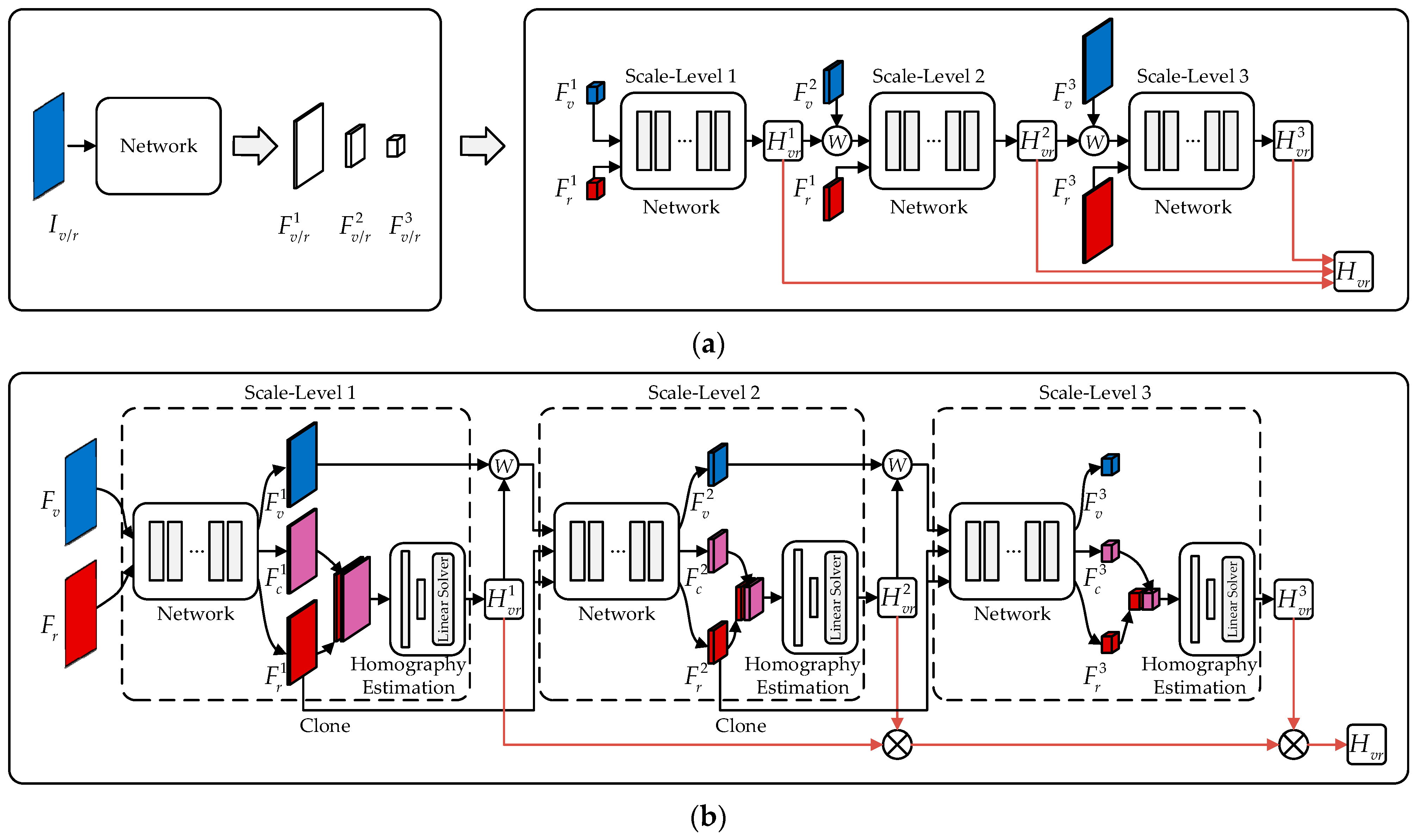
- We propose a novel coarse-to-fine strategy that obtains multi-scale feature maps through different stages in the regression network, thus avoiding the additional introduction of neural network structures and eliminating the need to design complex homography matrix fusion strategies.
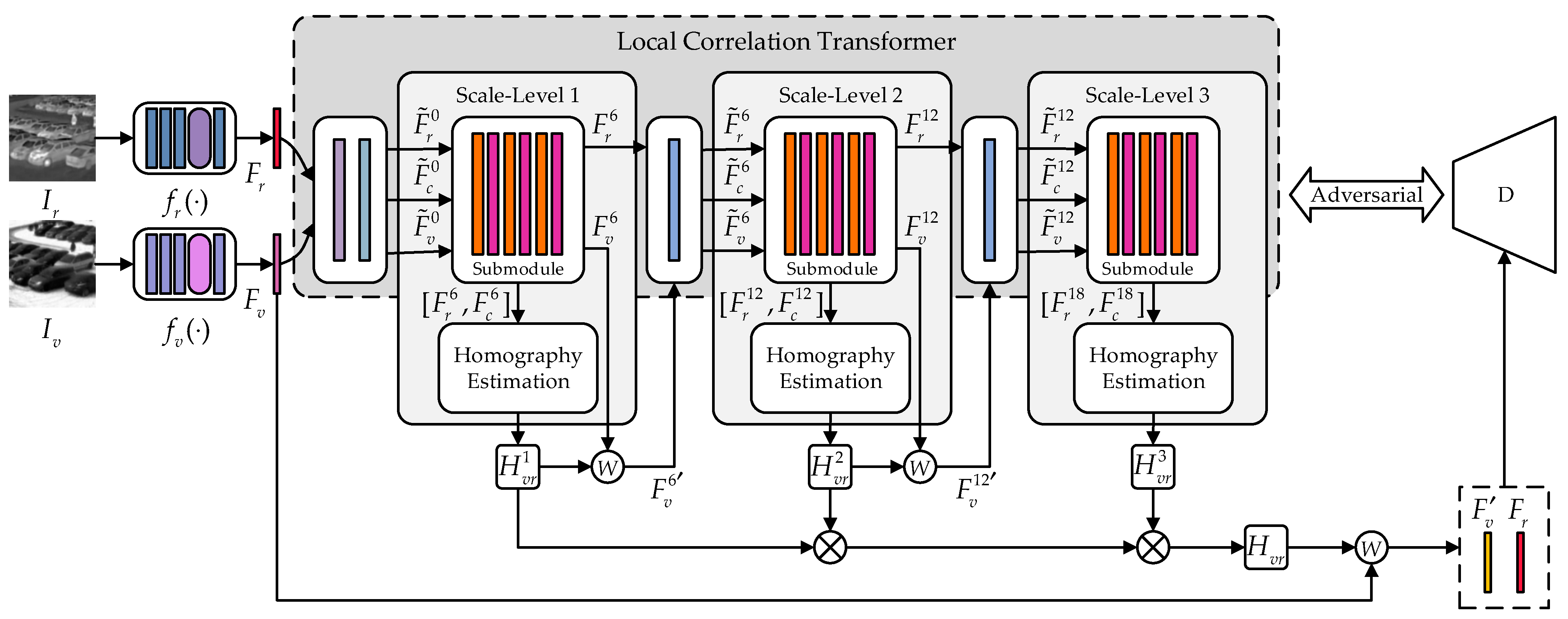
- We design a local correlation transformer with a self-attention layer to highlight important features for homography estimation. Each of its submodules also serves as a component at different scales in the coarse-to-fine strategy, aiming to obtain multi-scale feature maps.
- We design an improved average feature correlation loss, which increases the robustness of the model by computing the average of the triple loss over all LCTrans blocks.
We organize the remainder of the paper as follows. In Section 2, we provide an overview of the research work related to our method, including traditional homography estimation, deep homography estimation, and the coarse-to-fine strategy in the deep method. Section 3 elaborates on the proposed coarse-to-fine strategy and LCTrans alongside a detailed depiction of the model’s loss function. Section 4 presents the experimental results and demonstrates the effectiveness of the proposed components through ablation analysis. Some discussions are presented in Section 5. Finally, Section 6 provides some conclusions.
2. Related Works
In this section, we provide a brief overview of related work on our method, including traditional homography estimation, deep homography estimation, and the coarse-to-fine strategy in deep homography estimation.
2.1. Traditional Homography Estimation
Traditional homography estimation methods can be broadly divided into three main steps. First, feature points need to be detected in the image using feature point extractors, including scale invariant feature transform (SIFT) [13], speeded up robust features (SURF) [14], oriented FAST and rotated BRIEF (ORB) [15], binary robust invariant scalable keypoints (BRISK) [30], accelerated-KAZE (AKAZE) [31], KAZE [32], locality preserving matching (LPM) [33], grid-based motion statistics (GMS) [34], boosted efficient binary local image descriptor (BEBLID) [35], learned invariant feature transform (LIFT) [36], SuperPoint [37], second-order similarity network (SOSNet) [38], and order-aware networks (OANs) [39]. Second, a set of corresponding feature point pairs is found by a feature-matching algorithm. To robustly estimate the homography matrix, it is common to employ robust estimation algorithms with outlier rejection, such as random sample consensus (RANSAC) [17], marginalizing sample consensus (MAGSAC) [18], and MAGSAC++ [19]. Finally, a DLT [16] is solved for the homography. Although these methods have proven effective in visible light scenes, they still exhibit sensitivity to image noise and viewpoint changes. In particular, the performance of these methods can be challenged in multimodal images, such as infrared and visible images, due to significant modal differences.
2.2. Deep Homography Estimation
Deep homography estimation methods can be categorized into two classes: supervised and unsupervised. Supervised methods typically rely on datasets with ground-truth labels for network training. DeTone et al. [22] were the pioneers of applying deep learning to the task of homography estimation, and their proposed method outperforms traditional approaches in robustness. However, supervised methods rely on a large amount of ground-truth labels, increasing the time and cost of data preparation. In contrast, unsupervised methods do not require pre-labeled ground-truth labels and are usually optimized by minimizing the photometric loss between two images. Nguyen et al. [40] proposed an unsupervised deep learning homography estimation algorithm that trains the network by minimizing the pixel-level intensity error. In addition, Zhang et al. [41] introduced a content-aware mask during the estimation process, which aims to reject outlier regions, making the network more focused on regions that can be successfully aligned by homography. As research has progressed, some novel strategies have emerged. For instance, Ye et al. [42] proposed a distinctive homography estimation method based on a weighted sum of eight predefined homography flow bases, contrasting with the traditional strategy of using four offset vectors. Nie et al. [43] designed a multigrid deep homography network capable of global and local multigrid homography estimation to address the parallax issue in images better.
It is noteworthy that the above methods are primarily designed for visible image pairs. However, when these methods are applied to infrared and visible images, some algorithms may have difficulty converging during training. Recently, this issue has received significant attention from researchers. Debaque et al. [44] presented a supervised and unsupervised deep homography model and verified its viability on infrared and visible datasets. Luo et al. [45] proposed a detail-aware deep homography estimation network to preserve more detailed information in infrared and visible images. To alleviate the impact of feature differences on homography estimation, they also proposed a multi-scale generative adversarial network-based method to self-optimize the homography matrix [46]. In addition, Wang et al. [29] proposed a feature correlation transformer method to explicitly guide feature matching in homography estimation tasks for infrared and visible images. In this paper, we present a novel coarse-to-fine method that aims to refine the homography matrix progressively.
2.3. Coarse-to-Fine Strategy in Deep Homography Estimation
In homography estimation tasks, the coarse-to-fine strategy is a prevalent practice. This strategy usually relies on feature pyramids [23,24,25], Siamese networks [26], or other complex deep neural networks [27,28] to obtain feature maps at different scales. In general, the initial prediction of the homography matrix is based on lower-resolution feature maps, which are further optimized using higher-resolution feature maps. First, feature pyramids are utilized in [23,24,25] to produce feature maps at three scales. The method at each scale utilizes the previous scale’s homography matrix to warp the current scale’s source feature map, and then the homography matrix of the corresponding scale is obtained based on the warped source map and target feature map. Second, [26] used a Siamese network to obtain multi-scale feature maps. The approach warps the source image by using the previous scale’s homography matrix at each scale to obtain the warped source image. The warped source image and target image are then fed into the Siamese network to generate feature maps at the corresponding scales. Finally, [27,28] obtain multi-scale feature maps through different stages in the deep neural network structure. The strategy of [28] is similar to that of [23,24,25], but it adopts a different approach to obtaining the multi-scale feature maps. However, the strategy of [27] is slightly different in that it does not apply the previous scale’s homography matrix to the current scale’s source feature map. While the above methods adopt a similar coarse-to-fine strategy, they usually require the design of additional neural network structures to acquire the multi-scale feature maps and complex fusion strategies to deal with the homography matrices at each scale. To tackle these challenges, we introduce a novel coarse-to-fine strategy.
3. Method
In this section, we present an overview of the proposed homography estimation method. Subsequently, we delineate the novel coarse-to-fine strategy and elucidate its two constituent components: the LCTrans submodule and the homography estimation module. Finally, we show some details of the loss function.
3.1. Overview
In this paper, we introduce a new coarse-to-fine homography estimation method. Given a pair of grey-scale image patches and of size , as inputs to the network, we predict a homography transformation from to , denoted as . First, we utilize the visible shallow feature extraction network and the infrared shallow feature extraction network [29] to transform and into the fine-feature mappings and , respectively. Then, and are input into LCTrans to obtain the different scales of the homography matrices. Specifically, the various stages (submodules) of LCTrans are considered components of different scale levels in the coarse-to-fine strategy, aiming to generate multi-scale feature maps of size where k denotes the scale level, . In different scales, we feed the projected and unprojected target feature maps into the homography estimation module after cascading them on the channels to obtain the homography matrices in the corresponding scales. Finally, we multiply the homography matrices at different scales to obtain the final homography matrix . We also introduce a discriminator (D) to optimize the final homography matrix further. Similarly, by swapping the input order of the image patches and , we obtain the homography matrix . Figure 2 illustrates the network structure of the proposed method.
Figure 2.
The overall architecture of the proposed coarse-to-fine homography estimation network. The network consists of three main modules: the shallow feature extraction network, the LCTrans, and the discriminator (D). Notably, the stages of LCTrans are considered components at different scale levels aiming to generate multi-scale feature maps.
3.2. Coarse-to-Fine Strategy
In this study, we adopted a coarse-to-fine strategy to refine the homography matrix. We consider the outputs of different stages (submodules) in LCTrans as feature maps at different scales. We first make a coarse estimate using the highest-resolution feature map. Subsequently, we use lower-resolution feature maps sequentially to progressively refine the homography matrix. This is intended to guarantee the introduction of more global information at each successive step, thus gradually improving the estimate’s accuracy. Each scale comprises two fundamental components, the LCTrans submodule and the homography estimation module, where the LCTrans submodule contains six LCTrans blocks.
At the -th scale, we first feed the source feature map () and the target feature maps ( and ) of size into the LCTrans submodule where denotes the ordinal number of the FCTrans block, ; and indicates a deep copy of . In the LCTrans submodule, we explicitly guide the feature matching by constantly querying the feature correlation between the source and target features, thus projecting the source image into the target image in the feature dimension. Then, the LCTrans submodule outputs the source feature map , the projected target feature map , and the unprojected target feature map in the -th scale. Finally, the feature map is constructed by concatenating and in the channel dimension. This feature map is fed to the homography estimation module to obtain 4 offset vectors (8 values). By utilizing the DLT [16], we further compute the homography matrix . The homography matrix is used to warp the source feature map to obtain the input at the next level, i.e.,
where is implemented by a spatial transformation network (STN) [47].
As the position information between and is no longer the same, we only input and into the patch merging module to obtain the feature maps and of size . We need to project the source image into the target image in the feature dimension, so we make a deep copy of to get . By feeding , , and into the submodule under the -th scale, we can obtain the feature maps , , and , which in turn produces the homography matrix . In this process, we compute the homography matrix between the warped source and the target feature maps such that the homography matrix obtained at the current stage is a refinement of the homography matrix of the previous stage. Similarly, the homography matrices can be obtained at all scales.
Traditional coarse-to-fine strategies typically apply the current scale’s homography matrix to the next scale’s source feature map, resulting in the need to design complex fusion strategies for homography matrices at different scales. In contrast, our strategy applies the current scale’s homography matrix to the current scale’s source feature map, resulting in a warped source feature map that is used to generate the next scale’s source feature map. The core idea of our strategy is to gradually refine the homography matrix by making the source and target feature maps progressively closer at each scale. Hence, we do not need to design a complicated fusion strategy and simply multiply all the homography matrices to obtain the final homography matrix . The process can be expressed as:
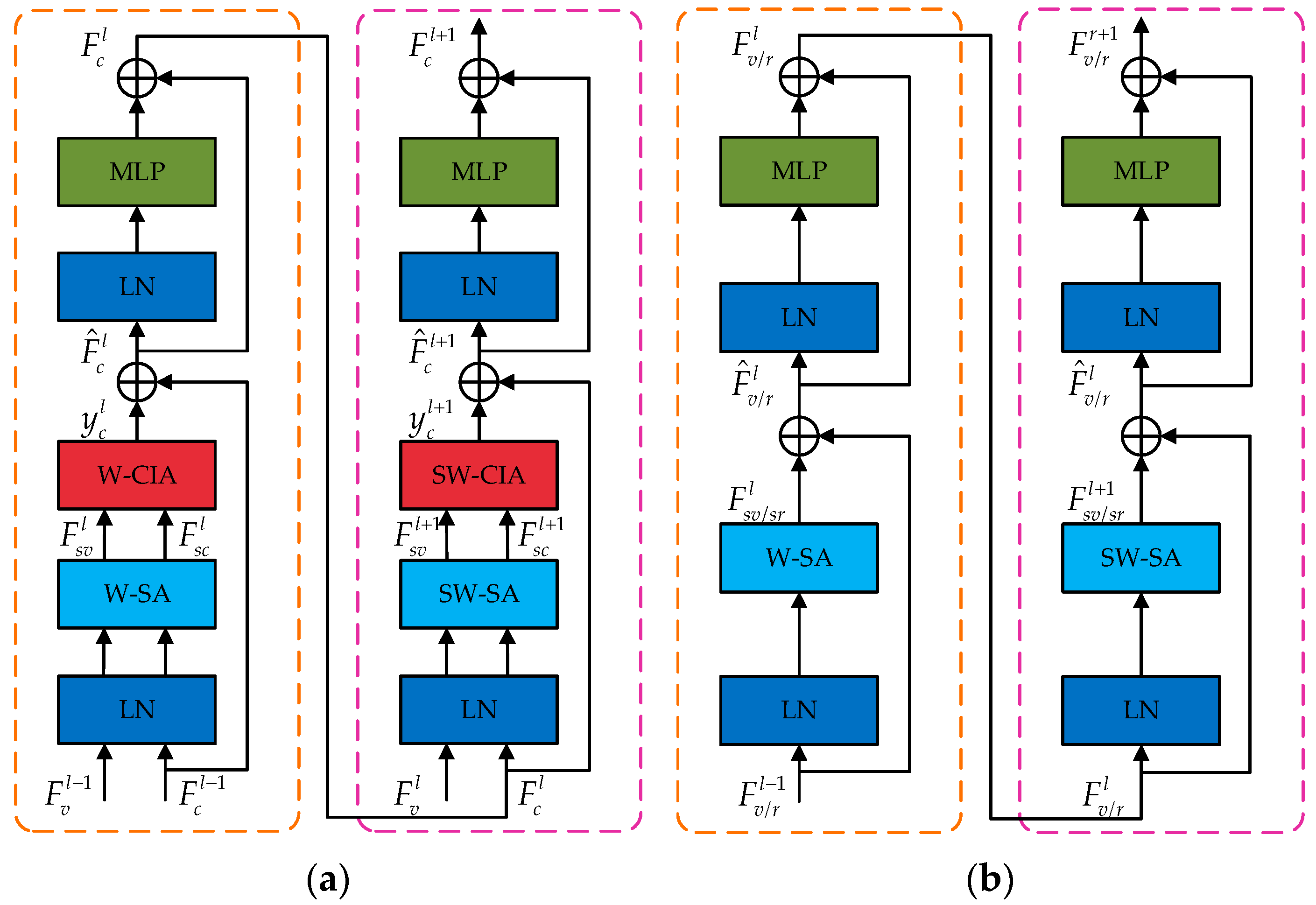
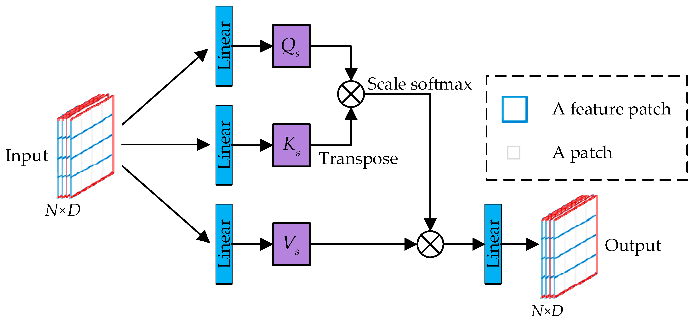
3.2.1. Local Correlation Transformer
FCTrans [29] recently achieved the homography estimation task for infrared and visible images through explicitly guided feature matching. Inspired by this work, we propose a further optimized framework, local correlation transformer (LCTrans), as shown in Figure 2. The framework aims to highlight important features more efficiently and thus improve the performance of homography estimation. The LCTrans framework consists of four main components: the patch partition module, the linear embedding module, the LCTrans submodule, and the patch merging module. Specifically, the different stages (submodules) in LCTrans are components of different scale levels from coarse-to-fine strategy. Each LCTrans submodule contains six LCTrans blocks, and the structure of two consecutive LCTrans blocks is shown in Figure 3.
Figure 3.
(a) Two consecutive LCTrans blocks for the projected target feature map. (b) Two consecutive LCTrans blocks for the source feature map and the unprojected target feature map. W-SA and SW-SA are self-attention modules with regular and shifted window configurations, respectively. W-CIA and SW-CIA are cross-image attention modules with regular and shifted window configurations, respectively. In particular, there is a patch merging module between the two submodules to halve the size of the feature map. Thus, the inputs to the first LCTrans block in the submodule are denoted as , , and , while the inputs to the remaining LCTrans blocks are denoted as , , and .
The LCTrans block is built by adding a (shifted) window self-attention module before the (shifted) window cross-image attention module in the FCTrans block while leaving the structure of the remaining layers unchanged. This design approach emphasizes significant features within the image, leading to a higher precision in homography estimation. Specifically, we first input , , and of size into the LayerNorm (LN) layer, respectively, and capture the relationships between the internal features of the image by the W-SA module, as shown in Figure 3a,b in the first LCTrans block. Second, a regular window partitioning strategy and a feature patch partitioning strategy are adopted to divide the feature map uniformly into windows of size containing feature patches. The feature patch size is , and the number of windows is . We flatten these windows in the feature patch dimension to obtain a window of size , where is , and is 4. This window of size is then fed into the W-SA module, as shown in Figure 4. Within this module, we obtain , , and through three separate linear layers. Our self-attention mechanism can be formulated as follows:
where indicates the dimensions of and , and represents the relative position bias of size and stands for the output of the W-SA module. A bias matrix, , is parameterized, and the values in are taken from .
Figure 4.
The architecture of the self-attention module.
Then, we take and of size as inputs to the W-CIA module to find the correlation between the source and target feature maps within the window, as shown in Figure 3a. To address the issue of vanishing gradients, we introduce residual connections following the W-CIA module. This procedure can be described as:
where is obtained by applying one linear layer to ; and are produced by applying two separate linear layers to , respectively; denotes the dimensions of and ; and represents the relative positional bias, which is the same as in the self-attention module. and before summing, the should first be resized to .
As the LCTrans block of and does not contain a W-CIA module, we add a residual connection after the W-SA module to alleviate the gradient vanishing, i.e.,
Finally, we feed , , and sequentially into the LayerNorm (LN) layer and the MLP module to generate the corresponding feature maps , , and . Similarly, we include a residual connection after the MLP module to address the issue of gradient vanishing. This process can be written as:
where indicates the operation of the LayerNorm layer and represents the operation of the MLP module.
The second LCTrans block is processed similarly to the above with one difference, i.e., it employs a shift window partitioning strategy [48].
3.2.2. Homography Estimation Module
At each scale level, the unprojected and projected target feature maps are connected in the channel dimension to serve as inputs to the homography estimation module. Our homography estimation module has a more straightforward structure and does not include convolutional layers, unlike the complex homography estimation module in the traditional coarse-to-fine strategy. The module comprises a LayerNorm layer, a global pooling layer, and a fully connected layer. The homography estimation module ultimately produces four offset vectors and acquires the homography matrix through DLT [16]. The whole process can be described by , i.e.,
where and denote the unprojected and the projected target feature maps output by the homography estimation module at the -th scale level, respectively.
3.3. Loss Function
In this section, we describe the loss functions of the generator and the discriminator in detail. The proposed AFCL is explained in the loss function of the generator.
3.3.1. Loss Function of the Generator
The generator’s loss function has four components: feature loss, average feature correlation loss (AFCL), adversarial loss, and homography loss. The feature loss [29] aims to promote the feature maps of the warped and target images to have similar data distributions and can be calculated as follows:
where represents the infrared feature map, denotes the visible feature map, and stands for the warped visible feature map.
The FCL [29] is obtained by summing the triple losses of all FCTrans blocks. However, as the number of FCTrans blocks increases, the FCL can increase significantly, decreasing robustness. Therefore, we introduce a novel constraint called average feature correlation loss (AFCL), which averages the triple loss of all LCTrans blocks in our method to increase the robustness of the model. AFCL is defined as follows:
where refers to the number of LCTrans blocks, which is set to 18 in the experiment; stands for the triplet loss produced by the l-th LCTrans block; , , and denote the source feature map, the projected target feature map, and the unprojected target feature map produced by the -th LCTrans block, respectively.
The adversarial loss [29] aims to minimize the difference between the warped and the target feature map, which can be expressed as:
where represents the probability that the warped feature map is similar to the target feature map. indicates the batch size. The homography matrix can be obtained by exchanging the input order of and . Following this operation, we can define and compute the loss , , and , similarly.
The homography loss [29] enforces and to be inverse matrices to each other and is written as:
where stands for the third-order identity matrix.
In summary, the generator’s loss function can be defined as:
where , , and refer to the weights of each item set, which are 0.5, 0.005, and 0.01, respectively.
3.3.2. Loss Function of the Discriminator
The discrimination aims to distinguish the warped feature maps from the target feature maps, and its loss function is as follows:
where and represent the losses between the target and the warped source feature maps.
The loss between the warped visible feature map and the target infrared feature map can be calculated as [29]:
where denotes the label of the target feature map, whose value is set as a random number from 0.95 to 1; represents the label of the warped source feature map, whose value is set as a random number from 0 to 0.05; ; and stand for the classification results of the discriminator to the target and the warped source feature maps, respectively. Similarly, another loss, , can be calculated by swapping the input order of and .
4. Experiments
In this section, we commence with a concise introduction to the dataset and experimental particulars. Subsequently, we provide a comprehensive exposition of the evaluation metrics employed in the experiments. Next, we conduct a comparative analysis, pitting our method against existing approaches using a synthetic benchmark dataset to substantiate its superior performance. Finally, we validate the efficacy of the proposed components through ablation studies.
4.1. Dataset and Experimentation Details
We have evaluated our method using a synthetic benchmark dataset [29,45,46]. This dataset consists of 49,738 training samples and 45 test samples, each containing unaligned infrared and visible image pairs of size . In particular, the test set offers the infrared ground-truth image for each image pair, allowing us to show the channel mixing results of the warped and ground-truth images in qualitative comparisons. For a more accurate assessment, the test set also provides four sets of truth-matched corner coordinates for each image pair.
During the training phase, we randomly cropped the image pairs into image patches of size as input to the network to increase the training data. Our network implementation was founded on the PyTorch (version number: 1.10.0) framework and trained on a computer equipped with an NVIDIA GeForce RTX 3090 (NVIDIA, Santa Clara, CA, USA) graphics card. The adaptive moment estimation (Adam) [49] optimizer was employed throughout the training process, initializing the learning rate at with a learning rate decay factor of 0.8 per epoch. To guarantee stable and efficient training of the generative adversarial network, we selected a batch size of 50. For the network parameter configuration of LCTrans, we set the window size to , the feature patch size to 2, the channel number in the first stage to , and the layer numbers in the submodule to {6, 6, 6}.
4.2. Evaluation Metric
To assess the effectiveness of our method, we utilize the corner error [23,26] as an evaluation metric. The corner error is calculated by computing the average distance between the corner points transformed by the estimated and ground-truth homography matrices. A lower error value indicates a better homography estimation performance. The corner error [23,26] can be defined as follows
where and are corner point transformed by the estimated homography and the ground-truth homography, respectively.
4.3. Comparison with Existing Methods
In this section, we first briefly introduce the comparison method. Then, we perform a qualitative and quantitative comparison between the proposed method and the comparison method, respectively, to demonstrate the performance of our method.
4.3.1. Comparative Methods
To comprehensively evaluate the performance of the proposed methods, we compare them with existing methods, including traditional feature-based and deep learning-based methods. Within the feature-based methods, we have selected eight methods for comparison, which are a combination of four feature extraction algorithms and two robust estimation algorithms. The feature extraction algorithms include SIFT [13], ORB [15], BRISK [30], and AKAZE [31], while the robust estimation algorithms include RANSAC [17] and MAGSAC++ [19]. In addition, the deep learning-based methods include the following four methods: CADHN [41], DADHN [45], HomoMGAN [46], and FCTrans [29].
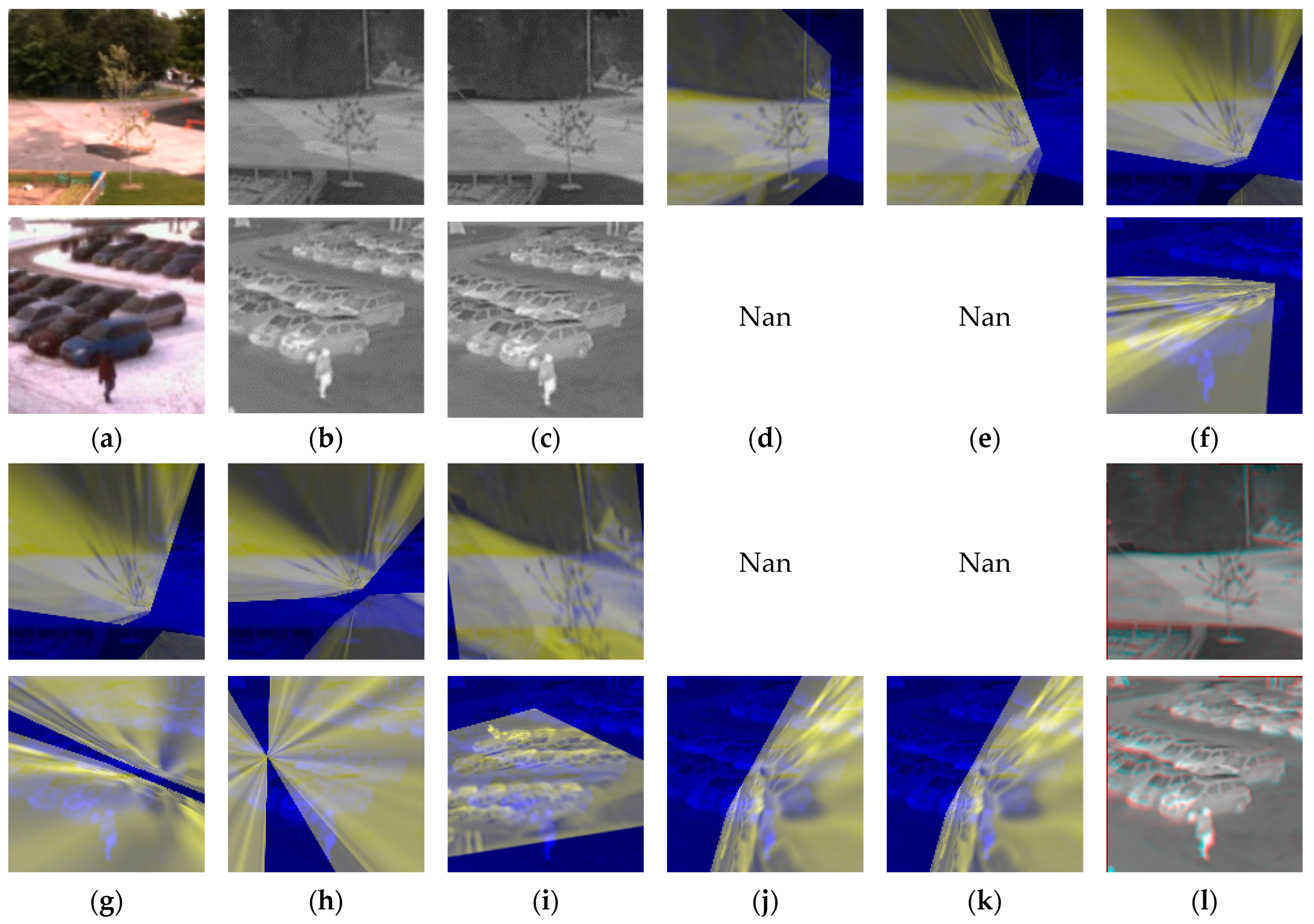
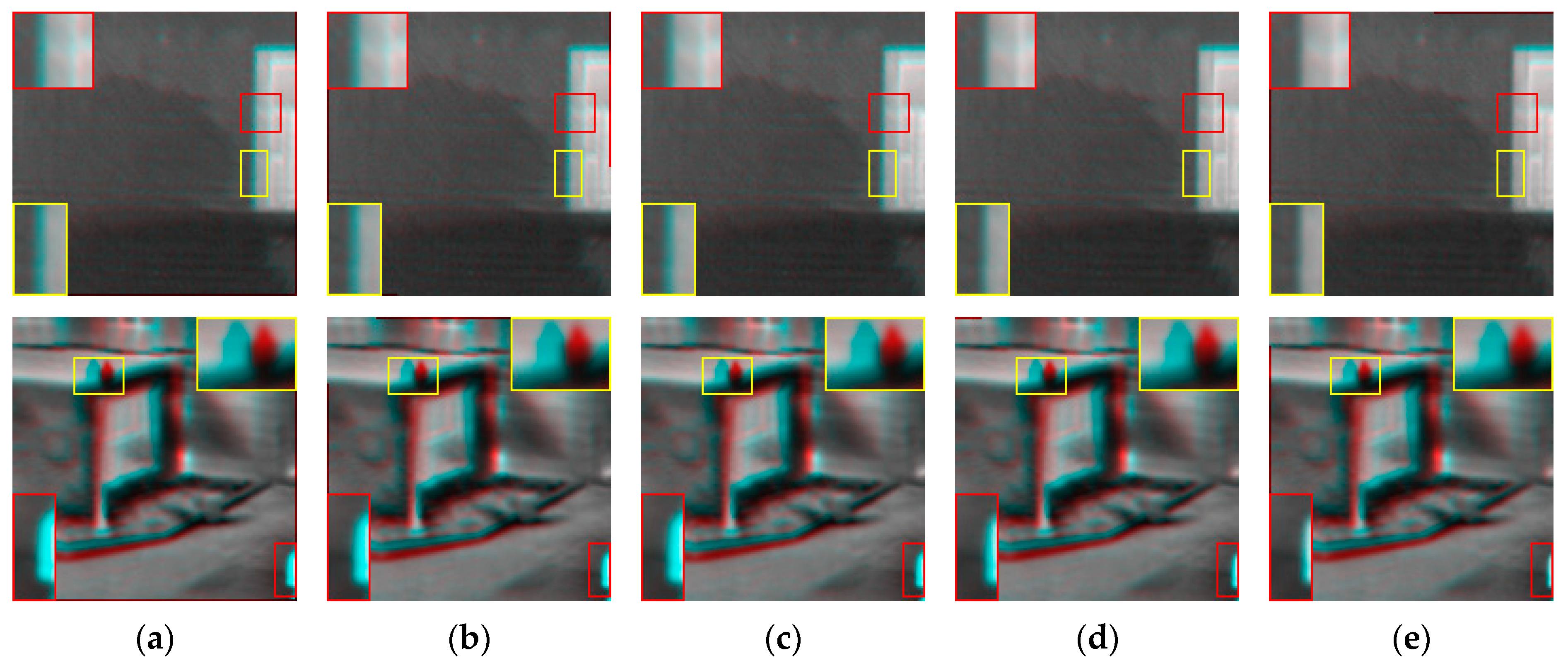
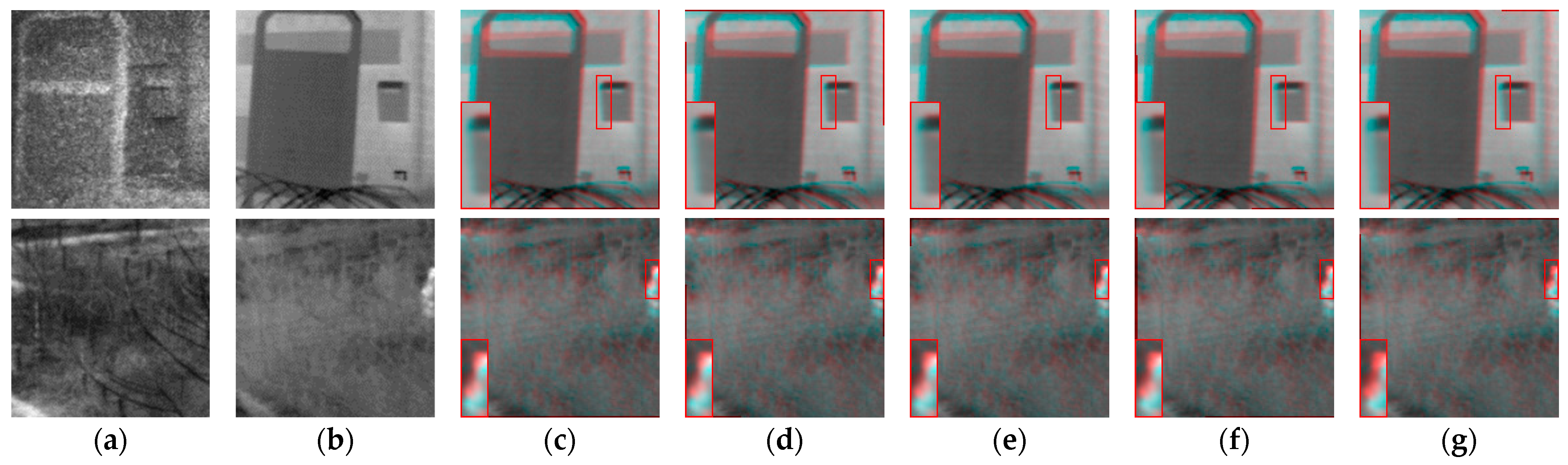
4.3.2. Qualitative Comparison
First, we compared the proposed method with the feature-based method, and the qualitative comparison results are shown in Figure 5. In Figure 5, “Nan” represents algorithmic failure, i.e., the method fails to compute the homography matrix successfully. Notably, both SIFT [13] and AKAZE [31] suffered an algorithmic failure in two examples, as shown in Figure 5d,e,j,k. While the other feature-based algorithms did not fail in these two examples, they still exhibited image distortion and ghosting to varying degrees. The common features between infrared and visible images suffer from high uncertainty; thus, feature-based methods’ performance is generally low. In contrast, our method presents considerable advantages in solving the homography estimation problem of infrared and visible images, significantly outperforming feature-based methods.
Figure 5.
Comparison with feature-based methods. (a) visible image; (b) infrared image; (c) ground-truth infrared image; (d) SIFT [13] + RANSAC [17]; (e) SIFT [13] + MAGSAC++ [19]; (f) ORB [15] + RANSAC [17]; (g) ORB [15] + MAGSAC++ [19]; (h) BRISAK [30] + RANSAC [17]; (i) BRISAK [30] + MAGSAC++ [19]; (j) AKAZE [31] + RANSAC [17]; (k) AKAZE [31] + MAGSAC++ [19]; and (l) the proposed algorithm. To achieve the above visualization results, we mix the blue and green channels of the warped infrared image with the red channel of the ground-truth infrared image, where the unaligned pixels appear as yellow, blue, red, or green ghosts. Notably, this approach is also used for all other visualization results.
Second, we conduct a qualitative comparison of the proposed method with the deep learning-based method, and the results are shown in Figure 6. While CADHN [41], DADHN [45], and HomoMGAN [46] perform well, green ghosting can still be seen in specific detail areas, including the edges of the door frame, the surface texture of the door, and the contours of the individual’s body, as shown in Figure 6a–c. In contrast, FCTrans [29] slightly outperforms CADHN [41], DADHN [45], and HomoMGAN [46] in these two examples. However, our method performs best and effectively reduces the ghosting phenomenon.
Figure 6.
Comparison with deep learning-based methods. From left to right: (a) CADHN [41]; (b) DADHN [45]; (c) HomoMGAN [46]; (d) FCTrans [29]; and (e) the proposed algorithm. We use red and yellow boxes to highlight error-prone regions and zoom them in for clearer comparison and analysis.
4.3.3. Quantitative Comparison
We report quantitative results for all compared methods in Table 1, where rows 3–10 are traditional feature-based methods, and rows 11–14 are deep learning-based methods. Notably, we introduce a reference term in row 2, representing identity transformation. The computed corner error reflects the original distance difference between point pairs. To present a thorough and hierarchical evaluation of the performance, we classify the test results into three difficulty levels based on the corner error: easy (top 0–30%), moderate (top 30–60%), and hard (top 60–100%). The average corner errors of all test images and the failure rate of the algorithm are shown in the last two columns of Table 1 where the failure rate is the number of test images in which the algorithm fails as a percentage of the total number of test images. In particular, “Nan” within the table indicates that no corner error data are available for that difficulty level. This is because the method experienced numerous failures in the test set, resulting in the absence of data at that level.
Table 1.
Quantitative results of the proposed algorithm and all compared methods.
From Table 1, we can see that our method achieves optimum performance. The average corner error decreases significantly from 4.91 to 4.80 compared with the second-best algorithm, FCTrans [29]. All feature-based methods present algorithmic failures, with average corner errors generally exceeding 100. Although the average corner error for SIFT [13] + RANSAC [17] is 50.87, which is superior to the other methods, its failure rate is the highest. This demonstrates that feature-based methods often have difficulty extracting or matching enough feature points in infrared and visible scenes, leading to algorithm failure or poor performance.
In contrast, the deep learning-based method significantly outperforms the feature-based method, with lower corner errors and no algorithmic failures. Specifically, CADHN [41], DADHN [45], HomoMGAN [46], and FCTrans [29] have exhibited superior performance on the test dataset, with average corner errors of 5.25, 5.08, 5.06, and 4.91, respectively. However, the proposed method performs better regarding difficulty levels and average corner error and significantly outperforms the other deep learning-based methods.
4.3.4. Failure Cases
Although the proposed method outperforms the other methods in the averaged corner error over all test images, it still performs poorly on some test images. Frequent algorithmic failures occur in feature-based methods, whose corner error is significantly higher than in deep learning-based methods. Hence, we have only conducted a failure case analysis for deep learning-based methods, and we present the corresponding visualization outcomes in Figure 7. To compare more intuitively, Table 2 lists the corresponding corner errors of each algorithm in the two cases.
Figure 7.
Comparison with deep learning-based methods on failure cases. From left to right: (a) visible image; (b) infrared image; (c) CADHN [38]; (d) DADHN [42]; (e) HomoMGAN [43]; (f) FCTrans [26]; (g) proposed algorithm. We use red boxes to highlight error-prone regions and zoom them in for clearer comparison and analysis.
Row 1 of Figure 7 shows that the DADHN [45] has less ghosting, and its visualization results are slightly better than the other algorithms. By comparing all the corner errors in row 2 of Table 2, we can see that DADHN [45] has the lowest corner error. However, the corner errors of the proposed method and FCTrans [29] are significantly higher than the rest of the algorithms, and both have comparable corner errors. This phenomenon could be ascribed to the necessity of both methods to search for the correlation between the source and target feature maps within a window. The presence of noise in the image significantly affects this process, leading to reduced performance in homography estimation.
As shown in row 2 of Figure 7, the proposed algorithm has slightly more ghosting than the others. Based on the results in row 3 of Table 2, FCTrans [29] demonstrates the smallest corner error while the proposed algorithm has the second smallest corner error. The lower quantity of common features between the source and target images in the second failure case is the reason for this outcome. The proposed method and FCTrans [29] are explicitly guided toward feature matching, making them more capable of model fitting than the other algorithms, so their corner errors are relatively small. Moreover, the proposed algorithm adopts a coarse-to-fine strategy and obtains the final homography matrix by multiplying the homography matrices at three scales. If the feature matching accuracy at one scale is insufficient, it will lead to insufficient accuracy of the homography matrix at that scale, which, in turn, will seriously degrade the performance of overall homography estimation. In contrast, FCTrans [29] does not adopt the coarse-to-fine strategy and uses more network layers to find the correlation between the source and target feature maps to obtain the homography matrix. Thus, FCTrans [29] has lower corner errors than the proposed method when there are insufficient common features of image pairs.
4.4. Ablation Studies
We conducted a series of ablation studies to verify the proposed components’ effectiveness. We focused on the following perspectives: the coarse-to-fine strategy, the self-attention mechanism, the submodule layer numbers, and the proposed AFCL.
4.4.1. Coarse-to-Fine
In the proposed method, we employ different stages (submodules) in LCTrans to obtain a multi-scale feature map, resulting in a stepwise refinement of the homography matrix. To demonstrate the effectiveness of the proposed coarse-to-fine strategy, we rely only on the last submodule to estimate the homography matrix, i.e., . The experimental results are shown in row 2 of Table 3. By comparing row 7 with row 2, we see that the average corner error increases from 4.80 to 4.96. This indicates the effectiveness of the coarse-to-fine strategy in achieving a progressive refinement of the homography matrix.
Table 3.
Results of ablation studies. Each row represents the result of a specific modification of our method. See the main text for further details.
4.4.2. Self-Attention
In the LCTrans block, we introduce self-attention to highlight the internal critical features of the image to improve the accuracy of homography estimation further. To verify self-attention effectiveness, we remove the self-attention layer in the LCTrans block in our experiments, and the results are shown in row 3 of Table 3. Comparing rows 7 and 3, we see that the average corner error increases from 4.80 to 4.86. Furthermore, to further demonstrate the efficacy of self-attention, we visualize the first channel of the output feature maps for each submodule, as shown in Figure 8. Compared with row 1 of Figure 8, the features presented in row 2 are significantly sparser. This demonstrates that self-attention helps capture feature relationships within the image more efficiently, thus highlighting features critical for homography estimation.
Figure 8.
Ablation study of self-attention. Row 1 represents the results after the model removes self-attention. Row 2 is the result of the model, including self-attention. From left to right: (a) infrared feature maps produced by the first submodule; (b) infrared feature maps produced by the second submodule; and (c) infrared feature maps produced by the third submodule. To facilitate visualization, the first channel of each submodule’s output feature map is selected and normalized so that the range of its pixel values is uniformly distributed between 0 and 255.
4.4.3. Layer Numbers
In the LCTrans framework, the output feature maps of different submodules are used to compute the homography matrix at different scales. To further analyze the effect of the submodule layer number on the homography estimation accuracy, we performed a series of ablation experiments. Specifically, we set the layer numbers of the submodules to {2, 2, 6}, {6, 2, 2}, and {6, 6, 6}, respectively, and compared their performance in homography estimation, as shown in rows 4, 5, and 7 of Table 3.
When the layer numbers were set to {2, 2, 6}, we observed the highest average of its corner error. This implies that when the layer numbers in the first submodule are relatively small, the model is likely to fail to adequately capture the basic structure and key information in the image, leading to an inaccurate initial estimation of the homography matrix, which further affects the overall performance. To overcome this limitation, we have increased the layer numbers in the first submodule to 6, e.g., the number of layers is set to {6, 2, 2}. By comparing row 4 with row 5, the average corner error decreases from 5.14 to 4.93. Nevertheless, by further comparing row 7 with row 5, we find that the average corner error increases from 4.80 to 4.93. This indicates that while the {6, 2, 2} setting succeeds in capturing more low-level features by increasing the layer numbers of the first submodule, the lower subsequent layer numbers lead to difficulties in fully extracting high-level features or more complex relationships. In contrast, the {6, 6, 6} setting maintains an overall deeper structure, ensuring that the model is able to fully extract and refine features at all levels.
4.4.4. AFCL
To verify the effectiveness of AFCL, we replace AFCL with FCL in our experiments, as shown in row 6 of Table 3. By contrasting rows 6 and 7, it becomes evident that the corner error average decreases significantly from 5.16 to 4.80. Therefore, this result suggests that the network can be trained more effectively by averaging all triple losses. Notably, the average corner error in row 6 is the highest of all the ablation studies, further demonstrating the effectiveness of AFCL.
5. Discussion
In this study, we proposed a novel coarse-to-fine homography estimation strategy. The traditional coarse-to-fine strategy usually relies on additional neural network structures and artificially designed fusion strategies to obtain multi-scale feature maps and to fuse homography matrices at different scales. While these approaches achieve superior performance, they undoubtedly increase the complexity of the network. Our strategy effectively reduces this complexity, simplifies the network structure, and outperforms existing methods in infrared and visible image scenes. By adopting this strategy, the model becomes easier to understand and implement and may provide a new solution idea for other related tasks. Moreover, our method also optimizes FCTrans [29] and FCL [29]. First, a local correlation transformer is designed, which highlights features important for solving homography estimation by adding a self-attention layer. Second, an average feature correlation loss is designed, which can effectively improve the robustness of the model.
Although the proposed method shows some superiority on synthetic benchmark datasets, through in-depth analysis and experimental validation, we find that the model’s performance still suffers from degradation when faced with specific challenging scenarios, e.g., more image noise and fewer common features between the source and target images. Specifically, the proposed method needs to find the correlation between the source and target feature maps within a window, so noise in the image can easily cause inaccurate feature matching, affecting the accurate estimation of the homography matrix. In situations with fewer common features, the proposed method improves the model fit by explicitly guiding feature matching, but the feature extraction capability at each scale is limited, which affects the accuracy of the homography matrix. Moreover, the generalization capability of our method on real datasets needs to be further improved.
To address the model’s limitations in some specific contexts, we aim to enhance the model by pursuing the following measures. First, we will further study more robust feature matching and correlation estimation methods to cope with image noise, such as adding noise suppression layers or adopting feature extraction and matching strategies more resistant to noise interference. Second, we plan to further optimize the LCTrans structure by introducing more contextual information or adjusting the work of the attention mechanism to improve the model’s performance in scenarios with insufficient common features. Finally, considering the diversity and complexity of real-world scenarios, we plan to introduce more real-world data for model training and validation to improve the model’s generalization ability.
6. Conclusions
In this paper, we have proposed a novel coarse-to-fine strategy for the homography estimation task of infrared and visible images. Compared with traditional methods, the proposed strategy obtains the multi-scale feature maps through different stages of the regression network instead of an additional neural network and avoids complex matrix fusion operations. Furthermore, we designed a local correlation transformer to highlight the critical features for solving homography estimation by introducing a self-attention layer where each submodule serves as a component of a different scale level in the coarse-to-fine strategy. To enhance the robustness of the model, we designed an average feature correlation loss. Extensive experimental results have demonstrated the effectiveness of all the newly proposed components, and the performance of our method outperforms existing methods in both quantitative and qualitative comparisons. Compared with the second-best method, FCTrans, the average corner error of the proposed method on the synthetic dataset decreases from 4.91 to 4.80.
However, the proposed method still has some limitations. For example, the method does not perform as well as some comparative methods on some of the test images in some challenging scenarios (image pairs with fewer common features or more image noise), and there is still room for improvement in its generalization ability on real-world datasets. Future research will focus on exploring more robust feature matching and correlation estimation methods, further optimizing the structure of the local correlation transformer, and considering introducing more real-world data for enhanced model training and validation to improve the model’s generalization ability.
Author Contributions
Conceptualization, X.W. and Y.L. (Yinhui Luo); methodology, X.W. and Y.L. (Yinhui Luo); software, X.W.; validation, X.W. and Y.L. (Yinhui Luo); formal analysis, X.W., Y.L. (Yinhui Luo), Q.F., Y.H. and C.S.; investigation, Y.W. and Y.L. (Yanhao Liao); resources, Y.L. (Yanhao Liao); data curation, Y.L. (Yanhao Liao); writing—original draft preparation, X.W. and Y.L. (Yinhui Luo); writing—review and editing, X.W., Y.L. (Yinhui Luo), Q.F., Y.H. and C.S.; visualization, X.W. and Y.L. (Yinhui Luo); supervision, C.S., Y.W. and Y.L. (Yanhao Liao); project administration, Y.W. and Y.L. (Yanhao Liao); funding acquisition, Y.L. (Yinhui Luo) and Q.F. All authors have read and agreed to the published version of the manuscript.
Funding
This research was funded in part by the National Key R&D Program of China (program no. 2021YFF0603904), in part by the Science and Technology Plan Project of Sichuan Province (program no. 2022YFG0027), in part by the Fundamental Research Funds for the Central Universities (program no. ZJ2022-004, and no. ZHMH2022-006), and in part by the College Students’ innovation and entrepreneurship training program of Civil Aviation Flight University of China (program no. 202310624020).
Acknowledgments
We sincerely thank the authors of CADHN for providing their algorithm codes to facilitate the comparative experiment. Meanwhile, we would like to thank the anonymous reviewers for their valuable suggestions, which were of great help in improving the quality of this paper.
Conflicts of Interest
The authors declare no conflict of interest.
Abbreviations
The following abbreviations are used in this manuscript:
| LCTrans | Local Correlation Transformer |
| AFCL | Average Feature Correlation Loss |
| DLT | Direct Linear Transformation |
| FCL | Feature Correlation Loss |
| SIFT | Scale Invariant Feature Transform |
| SURF | Speeded Up Robust Features |
| ORB | Oriented FAST and Rotated BRIEF |
| BRISK | Binary Robust Invariant Scalable Keypoints |
| AKAZE | Accelerated-KAZE |
| LPM | Locality Preserving Matching |
| GMS | Grid-Based Motion Statistics |
| BEBLID | Boosted Efficient Binary Local Image Descriptor |
| LIFT | Learned Invariant Feature Transform |
| SOSNet | Second-Order Similarity Network |
| OANs | Order-Aware Networks |
| RANSAC | Random Sample Consensus |
| MAGSAC | Marginalizing Sample Consensus |
| STN | Spatial Transformation Network |
| W-SA | Self-Attention with Regular Window |
| SW-SA | Self-Attention with Shifted Window |
| W-CIA | Cross-Image Attention with Regular Window |
| SW-CIA | Cross-Image Attention with Shifted Window |
| Adam | Adaptive Moment Estimation |
References
- Nie, L.; Lin, C.; Liao, K.; Liu, M.; Zhao, Y. A view-free image stitching network based on global homography. J. Vis. Commun. Image Represent. 2020, 73, 102950. [Google Scholar] [CrossRef]
- Huang, C.; Pan, X.; Cheng, J.; Song, J. Deep Image Registration with Depth-Aware Homography Estimation. IEEE Signal Process. Lett. 2023, 30, 6–10. [Google Scholar] [CrossRef]
- Lin, Y.; Wu, F.; Zhao, J. Reinforcement learning-based image exposure reconstruction for homography estimation. Appl. Intell. 2023, 53, 15442–15458. [Google Scholar] [CrossRef]
- Son, D.-M.; Kwon, H.-J.; Lee, S.-H. Visible and Near Infrared Image Fusion Using Base Tone Compression and Detail Transform Fusion. Chemosensors 2022, 10, 124. [Google Scholar] [CrossRef]
- Liu, C.; Feng, Q.; Sun, Y.; Li, Y.; Ru, M.; Xu, L. YOLACTFusion: An instance segmentation method for RGB-NIR multimodal image fusion based on an attention mechanism. Comput. Electron. Agric. 2023, 213, 108186. [Google Scholar] [CrossRef]
- Gao, X.; Shi, Y.; Zhu, Q.; Fu, Q.; Wu, Y. Infrared and Visible Image Fusion with Deep Neural Network in Enhanced Flight Vision System. Remote Sens. 2022, 14, 2789. [Google Scholar] [CrossRef]
- Xie, T.; Zhang, W. Fast Intrusion Detection in High Voltage Zone of Electric Power Operations Based on YOLO and Homography Transformation Algorithm. In Proceedings of the 2023 5th Asia Energy and Electrical Engineering Symposium (AEEES), Chengdu, China, 23–26 March 2023; pp. 686–691. [Google Scholar]
- Deng, H.; Ou, Z.; Zhang, G.; Deng, Y.; Tian, M. BIM and Computer Vision-Based Framework for Fire Emergency Evacuation Considering Local Safety Performance. Sensors 2021, 21, 3851. [Google Scholar] [CrossRef]
- Nath, N.D.; Cheng, C.S.; Behzadan, A.H. Drone mapping of damage information in GPS-Denied disaster sites. Adv. Eng. Inform. 2022, 51, 101450. [Google Scholar] [CrossRef]
- Ahmadi, S.S.; Khotanlou, H. A hybrid of inference and stacked classifiers to indoor scenes classification of rgb-d images. In Proceedings of the 2022 International Conference on Machine Vision and Image Processing (MVIP), Ahvaz, Iran, 23–24 February 2022; pp. 1–6. [Google Scholar]
- Singh, D.; Mohtasebi, M.; Chen, L.; Huang, C.; Mazdeyasna, S.; Fathi, F.; Yu, G. A fast algorithm towards real-time laser speckle contrast imaging. J. Biomed. Opt. 2022, 15, 011109. [Google Scholar]
- Rezaei, M.; Rastgoo, R.; Athitsos, V. TriHorn-Net: A model for accurate depth-based 3D hand pose estimation. Expert Syst. Appl. 2023, 223, 119922. [Google Scholar] [CrossRef]
- Lowe, D.G. Distinctive image features from scale-invariant keypoints. Int. J. Comput. Vis. 2004, 60, 91–110. [Google Scholar] [CrossRef]
- Bay, H.; Tuytelaars, T.; Gool, L.V. Surf: Speeded Up Robust Features. In Proceedings of the European Conference on Computer Vision, Graz, Austria, 7–13 May 2006; pp. 404–417. [Google Scholar]
- Rublee, E.; Rabaud, V.; Konolige, K.; Bradski, G. ORB: An Efficient Alternative to SIFT or SURF. In Proceedings of the 2011 International Conference on Computer Vision, Barcelona, Spain, 6–13 November 2011; pp. 2564–2571. [Google Scholar]
- Hartley, R.; Zisserman, A. Multiple View Geometry in Computer Vision; Cambridge University Press: Cambridge, UK, 2003. [Google Scholar]
- Fischler, M.A.; Bolles, R.C. Random sample consensus: A paradigm for model fitting with applications to image analysis and automated cartography. Commun. ACM 1981, 24, 381–395. [Google Scholar] [CrossRef]
- Barath, D.; Matas, J.; Noskova, J. MAGSAC: Marginalizing Sample Consensus. In Proceedings of the IEEE/CVF Conference on Computer Vision and Pattern Recognition, Long Beach, CA, USA, 15–20 June 2019; pp. 10197–10205. [Google Scholar]
- Barath, D.; Noskova, J.; Ivashechkin, M.; Matas, J. MAGSAC++, a Fast, Reliable and Accurate Robust Estimator. In Proceedings of the IEEE/CVF Conference on Computer Vision and Pattern Recognition, Seattle, WA, USA, 14–19 June 2020; pp. 1304–1312. [Google Scholar]
- Ma, J.; Tang, L.; Xu, M.; Zhang, H.; Xiao, G. STDFusionNet: An infrared and visible image fusion network based on salient target detection. IEEE Trans. Instrum. Meas. 2021, 70, 1–13. [Google Scholar] [CrossRef]
- Yu, K.; Xu, C.; Ma, J.; Fang, B.; Ding, J.; Xu, X.; Bao, X.; Qiu, S. Automatic Matching of Multimodal Remote Sensing Images via Learned Unstructured Road Feature. Remote Sens. 2022, 14, 4595. [Google Scholar] [CrossRef]
- DeTone, D.; Malisiewicz, T.; Rabinovich, A. Deep image homography estimation. arXiv 2016, arXiv:1606.03798. [Google Scholar]
- Le, H.; Liu, F.; Zhang, S.; Agarwala, A. Deep Homography Estimation for Dynamic Scenes. In Proceedings of the IEEE/CVF Conference on Computer Vision and Pattern Recognition, Seattle, WA, USA, 14–19 June 2020; pp. 7652–7661. [Google Scholar]
- Hong, M.; Lu, Y.; Ye, N.; Lin, C.; Zhao, Q.; Liu, S. Unsupervised Homography Estimation with Coplanarity-Aware GAN. In Proceedings of the IEEE/CVF Conference on Computer Vision and Pattern Recognition, New Orleans, LA, USA, 19–24 June 2022; pp. 17663–17672. [Google Scholar]
- Hou, B.; Ren, J.; Yan, W. Unsupervised Multi-Scale-Stage Content-Aware Homography Estimation. Electronics 2023, 12, 1976. [Google Scholar] [CrossRef]
- Shao, R.; Wu, G.; Zhou, Y.; Fu, Y.; Fang, L.; Liu, Y. Localtrans: A Multiscale Local Transformer Network for Cross-Resolution Homography Estimation. In Proceedings of the IEEE/CVF International Conference on Computer Vision, Montreal, QC, Canada, 10–17 October 2021; pp. 14890–14899. [Google Scholar]
- Li, Y.; Chen, K.; Sun, S.; He, C. Multi-scale homography estimation based on dual feature aggregation transformer. IET Image Process. 2023, 17, 1403–1416. [Google Scholar] [CrossRef]
- Huo, M.; Zhang, Z.; Yang, X. AbHE: All Attention-based Homography Estimation. arXiv 2022, arXiv:2212.03029. [Google Scholar]
- Wang, X.; Luo, Y.; Fu, Q.; Rui, Y.; Shu, C.; Wu, Y.; He, Z.; He, Y. Infrared and Visible Image Homography Estimation Based on Feature Correlation Transformers for Enhanced 6G Space–Air–Ground Integrated Network Perception. Remote Sens. 2023, 15, 3535. [Google Scholar] [CrossRef]
- Leutenegger, S.; Chli, M.; Siegwart, R.Y. BRISK: Binary Robust Invariant Scalable Keypoints. In Proceedings of the 2011 International Conference on Computer Vision, Barcelona, Spain, 6–13 November 2011; pp. 2548–2555. [Google Scholar]
- Alcantarilla, P.F.; Solutions, T. Fast explicit diffusion for accelerated features in nonlinear scale spaces. IEEE Trans. Patt. Anal. Mach. Intell 2011, 34, 1281–1298. [Google Scholar]
- Alcantarilla, P.F.; Bartoli, A.; Davison, A.J. KAZE Features. In Proceedings of the Computer Vision–ECCV 2012: 12th European Conference on Computer Vision, Florence, Italy, 7–13 October 2012; pp. 214–227. [Google Scholar]
- Ma, J.; Zhao, J.; Jiang, J.; Zhou, H.; Guo, X. Locality preserving matching. Int. J. Comput. Vis. 2019, 127, 512–531. [Google Scholar] [CrossRef]
- Bian, J.W.; Lin, W.Y.; Matsushita, Y.; Yeung, S.K.; Nguyen, T.D.; Cheng, M.M. Gms: Grid-Based Motion Statistics for Fast, Ultra-Robust Feature Correspondence. In Proceedings of the IEEE Conference on Computer Vision and Pattern Recognition, Honolulu, HI, USA, 21–26 July 2017; pp. 4181–4190. [Google Scholar]
- Suárez, I.; Sfeir, G.; Buenaposada, J.M.; Baumela, L. BEBLID: Boosted efficient binary local image descriptor. Pattern Recognit. Lett. 2020, 133, 366–372. [Google Scholar] [CrossRef]
- Yi, K.M.; Trulls, E.; Lepetit, V.; Fua, P. Lift: Learned Invariant Feature Transform. In Proceedings of the Computer Vision–ECCV 2016: 14th European Conference, Amsterdam, The Netherlands, 10–16 October 2016; pp. 467–483. [Google Scholar]
- DeTone, D.; Malisiewicz, T.; Rabinovich, A. Superpoint: Self-Supervised Interest Point Detection and Description. In Proceedings of the IEEE Conference on Computer Vision and Pattern Recognition Workshops, Salt Lake City, UT, USA, 18–22 June 2018; pp. 224–236. [Google Scholar]
- Tian, Y.; Yu, X.; Fan, B.; Wu, F.; Heijnen, H.; Balntas, V. Sosnet: Second Order Similarity Regularization for Local Descriptor Learning. In Proceedings of the IEEE/CVF Conference on Computer Vision and Pattern Recognition, Long Beach, CA, USA, 15–20 June 2019; pp. 11016–11025. [Google Scholar]
- Zhang, J.; Sun, D.; Luo, Z.; Yao, A.; Zhou, L.; Shen, T.; Chen, Y.; Quan, L.; Liao, H. Learning Two-View Correspondences and Geometry Using Order-Aware Network. In Proceedings of the IEEE/CVF International Conference on Computer Vision, Seoul, Republic of Korea, 27 October–2 November 2019; pp. 5845–5854. [Google Scholar]
- Nguyen, T.; Chen, S.W.; Shivakumar, S.S.; Taylor, C.J.; Kumar, V. Unsupervised deep homography: A fast and robust homography estimation model. IEEE Robot. Autom. Lett. 2018, 3, 2346–2353. [Google Scholar] [CrossRef]
- Zhang, J.; Wang, C.; Liu, S.; Jia, L.; Ye, N.; Wang, J.; Zhou, J.; Sun, J. Content-Aware Unsupervised Deep Homography Estimation. In Proceedings of the Computer Vision–ECCV 2020: 16th European Conference, Glasgow, UK, 23–28 August 2020; pp. 653–669. [Google Scholar]
- Ye, N.; Wang, C.; Fan, H.; Liu, S. Motion Basis Learning for Unsupervised Deep Homography Estimation with Subspace Projection. In Proceedings of the IEEE/CVF International Conference on Computer Vision, Montreal, QC, Canada, 10–17 October 2021; pp. 13117–13125. [Google Scholar]
- Nie, L.; Lin, C.; Liao, K.; Liu, S.; Zhao, Y. Depth-aware multi-grid deep homography estimation with contextual correlation. IEEE Trans. Circuits Syst. Video Technol. 2021, 32, 4460–4472. [Google Scholar] [CrossRef]
- Debaque, B.; Perreault, H.; Mercier, J.P.; Drouin, M.A.; David, R.; Chatelais, B.; Duclos-Hindié, N.; Roy, S. Thermal and visible image registration using deep homography. In Proceedings of the 2022 25th International Conference on Information Fusion (FUSION), Linköping, Sweden, 4–7 July 2022; pp. 1–8. [Google Scholar]
- Luo, Y.; Wang, X.; Wu, Y.; Shu, C. Detail-Aware Deep Homography Estimation for Infrared and Visible Image. Electronics 2022, 11, 4185. [Google Scholar] [CrossRef]
- Luo, Y.; Wang, X.; Wu, Y.; Shu, C. Infrared and Visible Image Homography Estimation Using Multiscale Generative Adversarial Network. Electronics 2023, 12, 788. [Google Scholar] [CrossRef]
- Jaderberg, M.; Simonyan, K.; Zisserman, A.; Kavukcuoglu, K. Spatial Transformer Networks. In Proceedings of the Advances in Neural Information Processing Systems, Montreal, QC, Canada, 7–12 December 2015; pp. 2017–2025. [Google Scholar]
- Liu, Z.; Lin, Y.; Cao, Y.; Hu, H.; Wei, Y.; Zhang, Z.; Lin, S.; Guo, B. Swin transformer: Hierarchical vision transformer using shifted windows. In Proceedings of the IEEE/CVF international conference on computer vision, Montreal, QC, Canada, 10–17 October 2021; pp. 10012–10022. [Google Scholar]
- Kingma, D.P.; Ba, J. Adam: A method for stochastic optimization. arXiv 2014, arXiv:1412.6980. [Google Scholar]
Disclaimer/Publisher’s Note: The statements, opinions and data contained in all publications are solely those of the individual author(s) and contributor(s) and not of MDPI and/or the editor(s). MDPI and/or the editor(s) disclaim responsibility for any injury to people or property resulting from any ideas, methods, instructions or products referred to in the content. |
© 2023 by the authors. Licensee MDPI, Basel, Switzerland. This article is an open access article distributed under the terms and conditions of the Creative Commons Attribution (CC BY) license (https://creativecommons.org/licenses/by/4.0/).