Abstract
This paper presents a new method for separating the mixed audio signals of simultaneous speakers using Blind Source Separation (BSS). The separation of mixed signals is an important issue today. In order to obtain more efficient and superior source estimation performance, a new algorithm that solves the BSS problem with Multi-Objective Optimization (MOO) methods was developed in this study. In this direction, we tested the application of two methods. Firstly, the Discrete Wavelet Transform (DWT) was used to eliminate the limited aspects of the traditional methods used in BSS and the small coefficients in the signals. Afterwards, the BSS process was optimized with the multi-purpose Strength Pareto Evolutionary Algorithm 2 (SPEA2). Secondly, the Minkowski distance method was proposed for distance measurement by using density information in the discrimination of individuals with raw fitness values for the concept of Pareto dominance. With this proposed method, the originals (original source signals) were estimated by separating the randomly mixed male and two female speech signals. Simulation and experimental results proved that the efficiency and performance of the proposed method can effectively solve BSS problems. In addition, the Pareto front approximation performance of this method also confirmed that it is superior in the Inverted Generational Distance (IGD) indicator.
1. Introduction
Blind Source Separation (BSS) has become an important analysis tool to differentiate signals from each other in subjects such as biomedical signal processing, image analysis and control systems [1]. BSS is the estimation of source signals from a set of mixed signals without knowledge of the source signals and their mixtures that make up this mixture [2]. Although single-objective and Multi-Objective Optimization (MOO) methods are used in this estimation process, the performance of single-objective optimization methods has not reached the desired level [3]. In BSS, efforts have been made to develop algorithms that perform well in different mixing models in order to obtain satisfactory separation performance [4]. Especially if there is noise in the source signals, the BSS process becomes much more difficult, so it has become compulsory to develop new techniques and algorithms [5].
In BSS, which is also a single-objective optimization method, the estimation of the source signals is provided by using the non-Gaussianity, sparsity and temporality properties of the signals. In single-objective optimization, while trying to reach a solution based on one of these features, the performance is increased by examining more than one feature with the use of Multi-Objective Optimization [6,7]. The performance of MOO methods used to separate mixed signals is often vital. Especially in biomedical signals, the accuracy of the signals separated using MOO methods is confirmed by at least two objective functions [8,9]. Many optimization algorithms have been proposed to separate the mixed signals with the BSS method. The mixed signals have been separated using the BSS method based on particle swarm optimization, but the convergence rate could not be brought to the desired level [10]. By basing the BSS method on the whale optimization algorithm, the complex parameter and convergence speed problem have been improved [11]. The artificial bee colony algorithm [12] and the hybrid invasive weed/biogeography-based optimization algorithm [13] have been actively applied to BSS problems. With the Multi-Objective BSS method (MO-BSS) [14], the ECG signal has been separated from the noise, and the performance rate of the algorithm in this area has subsequently been increased with the developed MO-BSS [15] by applying preprocessing. Shi et al. [16] have proposed an MOO algorithm using independent component analysis, and a different MOO algorithm technique using principal component analysis has been proposed by Xu et al. [17]. A new MOO method has been proposed for heart rate estimation, which is widely used in the biomedical field [18]. These are popular BSS methods, each based on a different MOO strategy. In addition to these studies, the Ensemble Empirical Mode Decomposition (EEMD) method has also been frequently used in signal separation in recent years [19].
In this study, simultaneously mixed speech sounds were separated. These speech sounds have been used as a guide in many areas that require analysis, such as communication, security, biomedical, control systems and intelligence. They are frequently used in applications such as coding and decoding speech signals for communication, speech sound recognition for security, disease diagnosis in biomedicine, speech disorders and correction, sound command control systems in the field of control and word capture in the field of intelligence. As a result of all these, we need to obtain the most original or closest-to-the-original speech signals in order to make a correct analysis. During speech or sound recording, noise interferes with signals due to many internal and external factors. Signals need to be separated from noise or other sounds for necessary analysis studies [20]. Although BSS operation is performed with SPEA2 in the method suggested by Pelegrina [14], the contributions of the present work are as follows:
- Wavelet transform is applied to a Strength Pareto Evolutionary Algorithm 2 (SPEA2)-based BSS algorithm. Signals are analyzed on the frequency axis and applied to MOO. Thus, a performance increase was achieved in the separation of signals. With this developed algorithm, Discrete Wavelet Transform (DWT) is applied to the signals, and a suitable method for the analysis of non-stationary signals is obtained. Due to these processes, although the data size is reduced, the calculation cost of the proposed method also decreases [21].
- Contrary to the traditional method, the distance between the points is calculated by the Minkowski distance in obtaining the Pareto curve. In the simulation results, it is seen that the use of Minkowski distance has a positive effect on the results.
- The success rate has been proven with Inverted Generational Distance (IGD), Hypervolume (HV) and Spread (Δ or SP) metrics, which are frequently used in the performance measurement of optimization algorithms.
- Extensive simulations are performed to compare the proposed scheme with some recent well-known BSS techniques in the literature, like EEMD. The proposed algorithm is also compared with a classical MOO-BSS algorithm.
2. Materials and Methods
2.1. Blind Source Separation
BSS is defined as the estimation of each source signal by separating the mixed signals from each other, without any information about either the source signals or how they are mixed with each other. The aim here is to find statistically independent signals within a given data set. In order to perform this operation, it is assumed that the sources are statistically independent of each other. According to these formulas, the mathematical representation of the mixture of independent source signals is as follows [22,23].
where , and are the observed/mixed signal vectors, the mixing matrix and the source signal vectors, respectively. Moreover, and indicate number of source signals and number of observed signals, respectively. BSS algorithms aim to find source signals from mixed signals. The BSS process is mathematically given by Equation (2) below:
where the vectors and are the estimated source signal vector and the mixing matrix, respectively. It is generally assumed that the number of signals observed in BSS algorithms is equal to the number of sources . In this case, is approximately the inverse of [24].
2.2. Multi-Objective Optimization
Optimally designed MOO methods are used for successful separation of mixed signals. By optimizing multiple objective functions at the same time, MOO generates solutions that can improve one objective without worsening another. An MOO problem with as the number of objective functions can be expressed as follows:
where , and denote the number of objective functions, feasible solution space and decision variables, respectively.
where and are inequality and equality constraints, respectively, while and are the number of inequality and equality constraints, respectively. When there are at least two objectives, for two solutions and , dominates if and only if is not worse than in all objectives and better than in at least one objective, if and only if
A solution is defined as a Pareto optimal solution if a solution does not exist that dominates [25,26,27,28].
2.3. SPEA2 and Minkowski Distance
The Strength Pareto Evolutionary Algorithm (SPEA) was developed by Zitzler et al. [29], which was then proposed as SPEA2 with necessary updates. The block diagram of this method is shown in Figure 1.
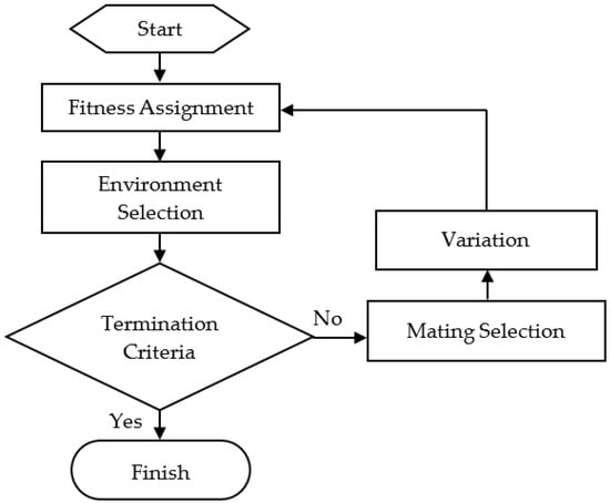
Figure 1.
Block diagram of SPEA2 algorithm.
In the SPEA2 algorithm, density information of individuals is needed to evaluate only dominant and non-dominant individuals. In Equation (7), the fitness function of individuals is
where and represent the original fitness of the i-th individual and the density of the i-th individual, respectively. The original conformity is expressed as
where and are the evolutionary population, external population and j-th individual’s strength value, respectively. This expression is mathematically defined as follows:
where defines the number of dominated solutions. In Equation (7), the density function of individuals is defined as follows:
where represents the Minkowski distance between two individuals [30,31]. It is suggested that the k-nearest neighbor method expression, which should be found, is obtained by the Minkowski distance method. It is widely used, especially for the classification of signals or finding optimal correlation. For the solutions we found, the normalization distance measurement expression with the Minkowski method is as follows:
where and are multidimensional points. is an integer and specifies the distance between two points of order [32,33].
After calculating the fitness of all solutions, the selection operator chooses an above-average solution, and standard steps are followed [29].
2.4. Objective Function Used in SPEA2
With the SPEA2 method, both objective functions are optimized simultaneously. The first of the two objective functions used in separating speech signals in SPEA2 is the function that handles the time-correlation properties of the signals. Optimization is provided by adapting this function to the minimization method. The aim here is to find the optimal solution by using the temporal feature of the resources with the first objective function (autocorrelation).
The second objective function is the -norm minimization method. This function is designed to consider the sparseness of resources. With sparseness, the goal is to deal with vectors where many elements are close to zero [14].
2.5. Ensemble Empirical Mode Decomposition (EEMD)
EEMD is a signal processing technique that has gained popularity in recent years due to its ability to decompose non-linear and non-stationary signals into their Intrinsic Mode Functions (IMFs). The basic function of EEMD is to generate multiple realizations of the signal by adding white noise to the original signal. Each realization is then decomposed using Empirical Mode Decomposition (EMD), which is a technique that extracts IMFs from a signal by iteratively sifting the signal and its envelopes. The IMFs are functions that have well-defined frequency ranges and represent the different scales of the signal.
The EMD process can be affected by noise and other artifacts, which can result in inaccurate decomposition. The addition of white noise in EEMD helps to overcome this problem by ensuring that each realization is different from the others, thus reducing the impact of noise and other artifacts on the decomposition.
A residue signal and the finite number of IMFs are decomposed as follows:
where is the final decomposed result, is the i-th IMF and is the residual component, which is the remaining item after the original signal has been reduced by the IMF [19,34,35,36].
2.6. Performance Metric
In order to quantitatively observe and evaluate the convergence of Multi-Objective Optimization (MOO) algorithms, Inverted Generational Distance IGD, Hypervolume (HV) and Spread (SP) methods are used as performance metrics [37]. Although each of the indicators in these methods is different, they all meet at a common point for convergence, spread and uniform distribution throughout the solution set [38].
2.6.1. Inverted Generational Distance
Let us assume that the IGD metric we use to measure the numerical performance of the algorithm has a set of properly distributed solutions on the real Pareto front. is the non-dominant set of solutions produced by the proposed method. The mean distance from to in IGD is defined as follows [37,39]:
where shows the minimum Euclidean distance between two points. The low calculated IGD value indicates the closeness of the distance between and [40,41].
2.6.2. Hypervolume
Hypervolume is one of the indicators that is frequently used in MOO algorithms and has a high computational cost due to its complexity [38,42]. The hypervolume performance metric is shown as follows:
where is termed the dominant hypervolume with respect to the reference point [40].
2.6.3. Spread
Spread measures the distribution and extent of the spread between solutions. Specifically, it gives the average of the Euclidean distances of the neighboring Pareto optimal solutions obtained as a result of the spread of solutions. When the distribution of Pareto optimal solutions is uniform, the spread is equal to zero. Spread is defined as follows [37,43]:
where , and denote the Euclidean distance between successive solutions, the mean of the Euclidean distance and the distance between the extreme solutions and , respectively [37].
3. Proposed Method
In signal separation applications, DWT can be used to separate features from time series and create an appropriate classification model [44]. It is a powerful and widely used signal processing tool for decomposing time-varying signals into frequency signals using scaling factors [45,46,47]. In the proposed algorithm, the mixed signals are filtered with DWT, and the Minkowski method is applied to measure the distance between two datasets on the Pareto front in SPEA2.
If all scales of the signals and the entire time span are used, the calculated coefficients will result in huge chunks of data. It becomes difficult to operate on all of these coefficients. In order to overcome this difficulty, conversion is made with the DWT method at a certain scale and position. The DWT method is expressed by Equation (17) [48] as follows:
where DWT is the observed data, is the scaling and is the translation parameter. If is the main wavelet, it is defined as follows [49]:
In DWT, approximation and detail coefficients of the signals are obtained with the help of low- and high-pass filters. The low- and high-pass filters are obtained with the help of a filter array during the scaling and transformation of the wavelet function. By increasing the conversion step, these processes continue until the desired separation level and the frequency resolution is thus increased [50]. When signals are filtered, data are lost. To minimize this loss, coefficients are determined to regain the original signal by using low- and high-pass filters. The approximation coefficients at the level and the detail coefficients are defined as follows [49,51]:
where and are low-pass and high-pass filters, respectively. In this study, the “db1” wavelet type from Daubechies wavelets is used to decompose the mixed signals.
4. Experimental Results
In this study, the DWT-MO-BSS method, which we proposed for the separation of mixed signals using the SPEA2 method, and the MO-BSS method have been compared (both methods are evolutionary algorithms). As a result of examining the signals in the frequency domain with the proposed method while they are in the time domain in MO-BSS, the comparison of the method in terms of performance and working time has been reported. In this study, male and female speech signals were randomly mixed and applied to the DWT-MOBSS algorithm, and its performance was tested. For this purpose, to measure the stability of the proposed algorithm, 50 Monte Carlo experiments were carried out by changing the random mixing matrix at each signal separation step. Parameter values used in the proposed SPEA2 simulation were population size 100, external set size 50, crossover rate 50 and maximum number of iterations 60.
Figure 2 shows the original male and two female speech signals used, randomly mixed forms of these three signals, and sample sizes of 4000 for the estimated source signals separated as a result of the MO-BSS algorithm. The original sounds used are taken from [52].
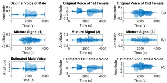
Figure 2.
Time-domain waveform of separated signals: (a) original signals, (b) mixture signals, and (c) estimated source signals.
Figure 3 shows the spectrogram of the estimated source signals as a result of separation with the original, mixed and proposed DWT-MOBSS method in the frequency space of the signals.
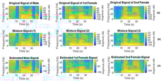
Figure 3.
Spectrogram of separated signals: (a) original signals, (b) mixture signals, and (c) estimated source signals.
In this study, feature reduction was obtained by applying the DWT method, and an appropriate classification model was created. Signals subjected to the DWT method were decomposed into their components by multiplying with the main wavelet, and as a result, no loss was experienced in the signals. As a result, significant gains in computational cost were achieved. As a result of the application of DWT in the male and two female speech signals we used, since the approaches give the original signal and the details give low-scale information, the approaches were separated into frequency coefficients with a low-pass filter up to the desired level. BSS was performed by applying the new signals obtained to the SPEA2 method.
The SNR measure was used to evaluate the accuracy and success rates of the experimental results, and analyses were made with IGD, HV and Δ metrics to measure the performance of the algorithm. The SNR measure is defined as follows:
where and represent the signal and the noise, respectively [53].
Mixed speech signals were separated by the proposed method for sample sizes of 2000, 4000, 6000, 8000, 10,000, 12,000 and 14,000. Table 1 shows the SNR results of the proposed method, EEMD with MO-BSS, for male and two female speech signals. As the table shows, while increasing the sample size does not affect the separation performance in MO-BSS, it increases the separation performance in EEMD and the proposed method. However, it should not be forgotten that increasing the sample length increases the separation time. Looking at the length of any sample in the table (8000), the proposed method separated all sounds very successfully compared to other methods. Moreover, male voice separation performance is the best of all three methods. This may be related to the frequency characteristics and probability distributions of the male voice. According to the table, the proposed method provided the best separation, followed by EEMD and MO-BSS. When the values in the table are examined, it can be seen that the proposed method is highly successful in both speech signals.

Table 1.
SNR values of male and female voice signals according to different sample sizes.
In addition, it is understood that the proposed method gives more stable results compared to the sample sizes. As shown in Figure 4, the male voice is better separated from the two female voice.
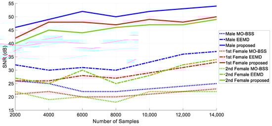
Figure 4.
SNR values of the MO-BSS and proposed algorithm.
It can be seen that the separated performance of MO-BSS is independent of the sample length. Monte Carlo analysis was performed by running these graphical algorithms 50 times with randomly selected mixing matrices [54]. Thus, the effect of different mixing matrices can be seen more clearly.
Performance metrics for MO-BSS are given in Table 2, EEMD in Table 3 and the proposed method in Table 4. The best, worst and average values of IGD, HV and SP are provided in these tables. In both algorithms, metric values have been obtained by running 50 times with sample sizes of 2000, 4000, 6000, 8000, 10,000, 12,000 and 14,000. Minimizing the performance metric in IGD and SP and maximizing the performance metric in HV shows the performance of the algorithm. According to the metrics, MO-BSS and EEMD performed worse than the proposed method. When looking at the average IGD, it increased with sample length. Similar rates can be seen in Table 2, Table 3 and Table 4. The different values in some sample sizes are related to the mixture matrices. For the HV metric, an increase was observed with sample length in all three tables. Increasing the sample length does not cause a change in the SP metric.
Table 2.
IGD, HV and SP metric values for the MO-BSS method.
Table 3.
IGD, HV and SP metric values for the EEMD method.
Table 4.
IGD, HV and SP metric values of the proposed method.
In the proposed method, although the processing load increased, a slight decrease in the calculation cost could be observed (Table 5). When these time values are interpreted with the increase in SNRs, it is clear that even the calculation cost for the proposed method is very advantageous. Table 5 shows that EEMD is quite advantageous in terms of computational cost. This is because EEMD can be considered a single-purpose optimization. It can be seen that the calculation times of MO-BSS and the proposed method are quite close to each other. The high calculation times for these methods are due to Multi-Objective Optimization. All these experiments were performed on MATLAB® R2021b.
Table 5.
Running times of algorithms according to different sample sizes.
5. Conclusions
Multi-Objective Optimization methods are used efficiently to increase the performance of blind resource allocation algorithms. This paper proposes both the DWT and the Minkowski distance method to separate mixed signals with the SPEA2 algorithm. At the same time, the proposed algorithm provides signal decomposition with two objective functions working simultaneously. The proposed DWT-MOBSS method has been found to be more efficient and advantageous when compared to the MO-BSS and EEMD algorithms. When the SNRs of the DWT-MOBSS algorithm are examined, its superiority is clearly revealed and the performance of the algorithm is supported by the performance metrics. Therefore, it can be used efficiently in BSS problems.
Author Contributions
Conceptualization, H.C.; methodology, H.C.; software, H.C.; validation, H.C. and N.K.; formal analysis, H.C. and N.K.; resources, H.C.; data curation, H.C.; writing—original draft preparation, H.C.; writing—review and editing, H.C. and N.K.; visualization, H.C.; project administration, N.K.; funding acquisition, H.C. and N.K. All authors have read and agreed to the published version of the manuscript.
Funding
The research was funded by the Erciyes University Scientific Research Projects Coordination Unit (FDK-2022-11706).
Data Availability Statement
The data presented in this study are available on request from the corresponding author.
Conflicts of Interest
The authors declare no conflict of interest.
References
- Jukiewicz, M.; Buchwald, M.; Cysewska-Sobusiak, A. Finding optimal frequency and spatial filters accompanying blind signal separation of EEG data for SSVEP-based BCI. Int. J. Electron. Telecommun. 2018, 4, 439–444. [Google Scholar] [CrossRef] [PubMed]
- Mahé, G.; Suzumura, G.G.; Moisan, L.; Suyama, R. A non-intrusive audio clarity index (NIAC) and its application to blind source separation. Signal Process. 2022, 194, 108448. [Google Scholar] [CrossRef]
- Ilgin, F.Y. Threshold optimisation with Bayesian approach in covariance absolute value detection method. Int. J. Electron. 2022, 109, 1680–1694. [Google Scholar] [CrossRef]
- Pelegrina, G.D.; Duarte, L.T. A multi-objective approach for post-nonlinear source separation and its application to ion-selective electrodes. IEEE Trans. Circuits Syst. II Express Briefs 2018, 65, 2067–2071. [Google Scholar] [CrossRef]
- Ghazdali, A.; Ourdou, A.; Hakim, M.; Laghrib, A.; Mamouni, N.; Metrane, A. Robust approach for blind separation of noisy mixtures of independent and dependent sources. Appl. Comput. Harmon. Anal. 2022, 60, 426–445. [Google Scholar] [CrossRef]
- Pelegrina, G.D.; Duarte, L.T. A multi-objective approach for blind source extraction. In Proceedings of the 2016 IEEE Sensor Array and Multichannel Signal Processing Workshop (SAM), Rio de Janeiro, Brazil, 10–13 July 2016; pp. 1–5. [Google Scholar]
- Mokriš, M. The independent component analysis with the linear regression–predicting the energy costs of the public sector buildings in Croatia. Croat. Oper. Res. Rev. 2022, 13, 173–185. [Google Scholar] [CrossRef]
- Li, D.; Wong, W.E.; Pan, S.; Koh, L.S.; Li, S.; Chau, M. Automatic test case generation using many-objective search and principal component analysis. IEEE Access 2022, 10, 85518–85529. [Google Scholar] [CrossRef]
- Sahin, O.; Akay, B.; Karaboga, D. Archive-based multi-criteria Artificial Bee Colony algorithm for whole test suite generation. Eng. Sci. Technol. Int. J. 2021, 24, 806–817. [Google Scholar] [CrossRef]
- Erkoc, M.E.; Karaboga, N. A comparative study of multi-objective optimization algorithms for sparse signal reconstruction. Artif. Intell. Rev. 2022, 55, 1–29. [Google Scholar] [CrossRef]
- Chu, D.; Chen, H.; Chen, H. Blind source separation based on whale optimization algorithm. MATEC Web Conf. 2018, 173, 03052. [Google Scholar]
- Wang, R. Blind source separation based on adaptive artificial bee colony optimization and kurtosis. Circuits Syst. Signal Process. 2021, 40, 3338–3354. [Google Scholar] [CrossRef]
- Ma, B.; Zhang, T. An analysis approach for multivariate vibration signals integrate HIWO/BBO optimized blind source separation with NA-MEMD. IEEE Access 2019, 7, 87233–87245. [Google Scholar] [CrossRef]
- Pelegrina, G.D.; Attux, R.; Duarte, L.T. Application of multi-objective optimization to blind source separation. Expert Syst. Appl. 2019, 131, 60–70. [Google Scholar] [CrossRef]
- Celik, H.; Karaboga, N. Blind Source Separation with Multi-Objective Optimization for Denoising. Elektron. Ir Elektrotechnika 2022, 28, 62–67. [Google Scholar] [CrossRef]
- Shi, Y.; Zeng, W.; Wang, N.; Zhao, L. A new method for independent component analysis with priori information based on multi-objective optimization. J. Neurosci. Methods 2017, 283, 72–82. [Google Scholar] [CrossRef] [PubMed]
- Xu, Y.; Wu, Z. Parameter identification of unsaturated seepage model of core rockfill dams using principal component analysis and multi-objective optimization. Structures 2022, 45, 145–162. [Google Scholar] [CrossRef]
- Macwan, R.; Benezeth, Y.; Mansouri, A. Heart rate estimation using remote photo plethysmography with multi-objective optimization. Biomed. Signal Process. Control 2019, 49, 24–33. [Google Scholar] [CrossRef]
- Elouaham, S.; Dliou, A.; Laaboubi, M.; Latif, R.; Elkamoun, N.; Zougagh, H. Filtering and analyzing normal and abnormal electromyogram signals. Indones. J. Electr. Eng. Comput. Sci. 2020, 20, 176–184. [Google Scholar] [CrossRef]
- Mitianoudis, N. Underdetermined Audio Source Separation Using Laplacian Mixture Modelling. In Blind Source Separation: Advances in Theory, Algorithms and Applications; Springer: Berlin/Heidelberg, Germany, 2014; pp. 197–229. [Google Scholar]
- Syed, S.H.; Muralidharan, V. Feature extraction using Discrete Wavelet Transform for fault classification of planetary gearbox–A comparative study. Appl. Acoust. 2022, 188, 108572. [Google Scholar] [CrossRef]
- Xu, C.; Ni, Y.Q.; Wang, Y.W. A novel Bayesian blind source separation approach for extracting non-stationary and discontinuous components from structural health monitoring data. Eng. Struct. 2022, 269, 114837. [Google Scholar] [CrossRef]
- Kervazo, C.; Bobin, J.; Chenot, C. Blind separation of a large number of sparse sources. Signal Process. 2018, 150, 157–165. [Google Scholar] [CrossRef]
- Cheriyan, M.M.; Michael, P.A.; Kumar, A. Blind source separation with mixture models—A hybrid approach to MR brain classification. Magn. Reson. Imaging 2018, 54, 137–147. [Google Scholar] [CrossRef] [PubMed]
- Kim, S.; Kim, I.; You, D. Multi-condition multi-objective optimization using deep reinforcement learning. J. Comput. Phys. 2022, 462, 111263. [Google Scholar] [CrossRef]
- Hancer, E.; Xue, B.; Zhang, M.; Karaboga, D.; Akay, B. Pareto front feature selection based on artificial bee colony optimization. Inf. Sci. 2018, 422, 462–479. [Google Scholar] [CrossRef]
- Xue, Y.; Li, M.; Shepperd, M.; Lauria, S.; Liu, X. A novel aggregation-based dominance for Pareto-based evolutionary algorithms to configure software product lines. Neurocomputing 2019, 364, 32–48. [Google Scholar] [CrossRef]
- Li, W.; Wang, R.; Zhang, T.; Ming, M.; Li, K. Reinvestigation of evolutionary many-objective optimization: Focus on the Pareto knee front. Inf. Sci. 2020, 522, 193–213. [Google Scholar] [CrossRef]
- Song, Y.; Fang, X. An Improved Strength Pareto Evolutionary Algorithm 2 with Adaptive Crossover Operator for Bi-Objective Distributed Unmanned Aerial Vehicle Delivery. Mathematics 2023, 11, 3327. [Google Scholar] [CrossRef]
- Yuan, X.; Zhang, B.; Wang, P.; Liang, J.; Yuan, Y.; Huang, Y.; Lei, X. Multi-objective optimal power flow based on improved strength Pareto evolutionary algorithm. Energy 2017, 122, 70–82. [Google Scholar] [CrossRef]
- Khanra, M.; Nandi, A.K. Optimal driving based trip planning of electric vehicles using evolutionary algorithms: A driving assistance system. Appl. Soft Comput. 2020, 93, 106361. [Google Scholar] [CrossRef]
- Xu, H.; Zeng, W.; Zeng, X.; Yen, G.G. An evolutionary algorithm based on Minkowski distance for many-objective optimization. IEEE Trans. Cybern. 2018, 49, 3968–3979. [Google Scholar] [CrossRef]
- Fu, C.; Jianhua, Y. Granular Classification for Imbalanced Datasets: A Minkowski Distance-Based Method. Algorithms 2021, 14, 54. [Google Scholar] [CrossRef]
- Li, C.; Tao, Y.; Ao, W.; Yang, S.; Bai, Y. Improving forecasting accuracy of daily enterprise electricity consumption using a random forest based on ensemble empirical mode decomposition. Energy 2018, 165, 1220–1227. [Google Scholar] [CrossRef]
- Elouaham, S.; Dliou, A.; Latif, R.; Laaboubi, M.; Zougagh, H.; Elkhadiri, K. Analysis Electroencephalogram Signals Using Denoising and Time-Frequency Techniques. Extraction 2021, 13, 14. [Google Scholar]
- Yang, Z.-X.; Zhong, J.-H. A Hybrid EEMD-Based SampEn and SVD for Acoustic Signal Processing and Fault Diagnosis. Entropy 2016, 18, 112. [Google Scholar] [CrossRef]
- Akay, B. Synchronous and asynchronous Pareto-based multi-objective artificial bee colony algorithms. J. Glob. Optim. 2013, 57, 415–445. [Google Scholar] [CrossRef]
- Sandoval, C.; Cuate, O.; González, L.C.; Trujillo, L.; Schütze, O. Towards fast approximations for the hypervolume indicator for multi-objective optimization problems by Genetic Programming. Appl. Soft Comput. 2022, 125, 109103. [Google Scholar] [CrossRef]
- Long, Q.; Li, G.; Jiang, L. A novel non-dominated sorting genetic algorithm for multi-objective optimization. J. Comput. Sci. 2021, 23, 31–43. [Google Scholar]
- Sun, Y.; Yen, G.G.; Yi, Z. IGD indicator-based evolutionary algorithm for many-objective optimization problems. IEEE Trans. Evol. Comput. 2018, 23, 173–187. [Google Scholar] [CrossRef]
- Yen, G.G.; He, Z. Performance metric ensemble for multiobjective evolutionary algorithms. IEEE Trans. Evol. Comput. 2013, 18, 131–144. [Google Scholar] [CrossRef]
- Tang, W.; Liu, H.L.; Chen, L.; Tan, K.C.; Cheung, Y.M. Fast hypervolume approximation scheme based on a segmentation strategy. Inf. Sci. 2020, 509, 320–342. [Google Scholar] [CrossRef]
- Mirjalili, S.; Lewis, A. Novel performance metrics for robust multi-objective optimization algorithms. Swarm Evol. Comput. 2015, 21, 1–23. [Google Scholar] [CrossRef]
- Bahoura, M.; Ezzaidi, H.; Méthot, J.F. Filter group delays equalization for 2D discrete wavelet transform applications. Expert Syst. Appl. 2022, 200, 116954. [Google Scholar] [CrossRef]
- Naseer, R.A.; Nasim, M.; Sohaib, M.; Younis, C.J.; Mehmood, A.; Alam, M.; Massoud, Y. VLSI architecture design and implementation of 5/3 and 9/7 lifting Discrete Wavelet Transform. Integration 2022, 87, 253–259. [Google Scholar] [CrossRef]
- Devi, D.; Sophia, S.; Prabhu, S.B. Deep learning-based cognitive state prediction analysis using brain wave signal. In Cognitive Computing for Human-Robot Interaction; Academic Press: Cambridge, MA, USA, 2021; pp. 69–84. [Google Scholar]
- Bendahane, B.; Jenkal, W.; Laaboubi, M.; Latif, R. HDL Coder Tool for ECG Signal Denoising. In International Conference on Digital Technologies and Applications; Springer Nature: Cham, Switzerland, 2023; pp. 753–760. [Google Scholar]
- Mota-Carmona, J.R.; Pérez-Escamirosa, F.; Minor-Martínez, A.; Rodríguez-Reyna, R.M. Muscle fatigue detection in upper limbs during the use of the computer mouse using discrete wavelet transform: A pilot study. Biomed. Signal Process. Control 2022, 76, 103711. [Google Scholar] [CrossRef]
- Shen, M.; Wen, P.; Song, B.; Li, Y. An EEG based real-time epilepsy seizure detection approach using discrete wavelet transform and machine learning methods. Biomed. Signal Process. Control 2022, 77, 103820. [Google Scholar] [CrossRef]
- Yesilli, M.C.; Chen, J.; Khasawneh, F.A.; Guo, Y. Automated Surface Texture Analysis via Discrete Cosine Transform and Discrete Wavelet Transform. Precis. Eng. 2022, 77, 141–152. [Google Scholar] [CrossRef]
- Dolatabadi, S.; Seyedi, H.; Tohidi, S. A new method for loss of excitation protection of synchronous generators in the presence of static synchronous compensator based on the discrete wavelet transform. Electr. Power Syst. Res. 2022, 209, 107981. [Google Scholar] [CrossRef]
- Voice Sources. Available online: https://www.kecl.ntt.co.jp/icl/signal/sawada/demo/bss2to4/index.html (accessed on 22 August 2023).
- Erkoc, M.E.; Karaboga, N. Sparse signal reconstruction by swarm intelligence algorithms. Eng. Sci. Technol. Int. J. 2021, 24, 319–330. [Google Scholar] [CrossRef]
- Hartland, N.P.; Maltoni, F.; Nocera, E.R.; Rojo, J.; Slade, E.; Vryonidou, E.; Zhang, C. A Monte Carlo global analysis of the Standard Model Effective Field Theory: The top quark sector. J. High Energy Phys. 2019, 1–78. [Google Scholar] [CrossRef]
Disclaimer/Publisher’s Note: The statements, opinions and data contained in all publications are solely those of the individual author(s) and contributor(s) and not of MDPI and/or the editor(s). MDPI and/or the editor(s) disclaim responsibility for any injury to people or property resulting from any ideas, methods, instructions or products referred to in the content. |
© 2023 by the authors. Licensee MDPI, Basel, Switzerland. This article is an open access article distributed under the terms and conditions of the Creative Commons Attribution (CC BY) license (https://creativecommons.org/licenses/by/4.0/).