A Novel Complex-Valued Hybrid Neural Network for Automatic Modulation Classification

Abstract

Currently, dealing directly with in-phase and quadrature time series data using the deep learning method is widely used in signal modulation classification. However, there is a relative lack of methods that consider the complex properties of signals. Therefore, to make full use of the inherent relationship between in-phase and quadrature time series data, a complex-valued hybrid neural network (CV-PET-CSGDNN) based on the existing PET-CGDNN network is proposed in this paper, which consists of phase parameter estimation, parameter transformation, and complex-valued signal feature extraction layers. The complex-valued signal feature extraction layers are composed of complex-valued convolutional neural networks (CNN), complex-valued gate recurrent units (GRU), squeeze-and-excite (SE) blocks, and complex-valued dense neural networks (DNN). The proposed network can improve the extraction of the intrinsic relationship between in-phase and quadrature time series data with low capacity and then improve the accuracy of modulation classification. Experiments are carried out on RML2016.10a and RML2018.01a. The results show that, compared with ResNet, CLDNN, MCLDNN, PET-CGDNN, and CV-ResNet models, our proposed complex-valued neural network (CVNN) achieves the highest average accuracy of 61.50% and 62.92% for automatic modulation classification, respectively. In addition, the proposed CV-PET-CSGDNN has a significant improvement in the misjudgment situation between 64QAM, 128QAM, and 256QAM compared with PET-CGDNN on RML2018.01a.

1. Introduction

Automatic modulation classification (AMC) plays a crucial role in the field of satellite communication, particularly when reliable prior information is not readily available [1,2]. In the past few years, various deep learning (DL) networks, such as convolutional neural networks (CNN), dense neural networks (DNN), residual neural networks (ResNet), and recurrent neural networks (RNN), have been used in the field of modulation classification because of their advantages of no manual feature extraction and high recognition accuracy [1,3,4,5,6]. The research on the application of DL in communication is relatively abundant; however, there are few examples considering complex representations of signal attributes [7]. Some existing DL-AMC models consider the real and imaginary components of complex-valued input as independent channels and do not fully exploit the inherent interactions between them, which could degrade the performance of the model and hinder its interpretability [7,8].

Usually, most of the collected signals, such as electromagnetic, optical waves, and RF signals, are complex numbers [9]. For example, in the actual situation, the modulation signal in the communication field is complex and consists of in-phase (I) and quadrature (Q) channel data, where the phase component represents the time course or position difference and the amplitude represents the energy or power of the wave [10,11,12]. Since complex-valued neural networks (CVNNs) can directly process phase and amplitude information and can completely extract wave information, the data expression ability can be improved by using CVNNs, which is more suitable for processing wave-related information processing models than real-valued neural networks (RVNNs) [13,14], and provides a new solution for dealing with problems with complex characteristics or calculations on a complex domain. Therefore, some researchers have researched CVNNs based on deep learning. In 1990, CVNNs were first formally described by Clarke [11]. In 1992, Hirose started to utilize complex weights and activation functions for building neural networks [15,16]. Later, Hirose et al. explained the mathematical expressions of complex numbers and connected them with the field of signal processing [11,17,18,19]. They found that CVNNs can achieve easier optimization [20], better generalization characteristics [19], faster learning [21], and allow for noise-robust memory mechanisms [22] compared with RVNNs. For example, Wisdom et al. [23] and Arjovsky et al. [21] proved that complex-valued RNNs could make the network have a richer representation ability. Danihelka et al. [22] introduced complex expression into the Long Short-Term Memory (LSTM) network and found that complex-valued LSTM had more advantages than real LSTM in retrieval and insertion of associative memory. Until 2018, Trabelsi et al. [24] provided the key components of CVNNs, which could realize convolution, activation, batch-normalization, and other operations on complex-valued input data, and applied them to vision tasks, music transcription, and speech spectrum prediction to achieve better performance than the corresponding RVNN. In the field of communication signals, complex-valued CNN has been applied to detect transmitted signals on spatial modulation [25], which could reduce the computational complexity by 14.71% compared to the traditional approach. According to Chang et al.’s research [26], signal equalization utilizing complex-valued CNN could restore communication signals from noisy signals affected by wireless channels. In 2020, Jakob Krzyston et al. [27] realized the calculation of complex convolution in real-valued deep learning frameworks by way of a linear combination of real convolution and two columns of real arrays. Compared with the RVNNs with the same number of parameters on RML2016.10a, the improvement in the recognition accuracy of the CVNN is more than 30% when the signal-to-noise ratio (SNR) level is below −5 dB. However, this method only solves the realization of complex convolution. At the same time, a complex-valued DNN is proposed, which has a lower error rate and fewer parameters than real-valued DNN and complex ResNets [5]. In 2022, to better improve the performance of the DL-AMC models based on CVNNs, S. Kim et al. [12] extended max-pooling and softmax to complex operations. To handle complex-valued data, complex-valued CNN and complex-valued ResNet were developed based on the basic architecture of real-valued CNN and ResNet. Compared with real-valued CNN and ResNet on different data, it is found that the proposed classifier improves the SMR performance. The performance of the phase-dependent modulation type is improved. Jie Xu et al. [28] proposed a complex-valued dense layer to realize the extraction of complex features when calculating classification results. And then complex-valued VGG and complex-valued ResNet are proposed and discussed for their applicability to signal modulation classification and UAV recognition. The results verify that, compared with the equivalent RVNNs, CVNNs have higher accuracy, lower computational complexity, and fewer model parameters.

Although researchers have researched CVNNs in signal processing, there is still a lack of CVNNs that can be used in signal modulation classification. Therefore, to make full use of the inherent relationship between in-phase and orthogonal time series data and enhance the feature extraction ability of the DL-AMC models for improving the accuracy of model recognition, we propose a complex-valued hybrid neural network. Based on the existing model in reference [29], the original in-phase and quadrature time series data were first processed by phase parameter estimation and transformation, and then the complex-valued signal feature extraction layers were used to extract the spatial and temporal characteristics of the signal for modulation signal recognition. The contributions of this paper are summarized as follows: (1) We propose a method to extend the Gate Recurrent Unit (GRU) to complex fields to reduce information loss in complex-valued input data; (2) to fully exploit the inherent interrelations in in-phase and quadrature time series data, we extend the PET-CGDNN model to the complex framework to realize complex operations; (3) to better learn the relationship between different channels and effectively extract the features of signal modulation classification, the squeeze-and-excite (SE) block as the attention mechanism is introduced in the feature extraction layer.

The remaining sections of this article are organized as follows: In Section 2, we introduce the signal model and provide an overview of complex-valued operation building blocks, which include the architecture and principles of complex convolution, complex batch-normalization, and other relevant modules. Then, we give the details of the proposed CV-PET-CSGDNN model. Section 3 presents the experimental setup and evaluation method. Furthermore, the experimental results of CV-PET-CSGDNN are analyzed and discussed in Section 4. Finally, in Section 5, we provide a summary of the key findings and offer insights into future directions for research in this field.

2. Signal Model and Proposed System Model

In this section, the complex-valued building blocks of CVNNs are presented, which include complex convolution, complex ReLU, complex GRU, and complex softmax. And then introduce our proposed complex-valued PET-CSGDNN model.

2.1. Signal Model

The complex baseband signal model, which includes I and Q components, can be represented as follows:

$$y(l)=A(l)e^{j(\omega l+\phi )}x(l)+n(l),\begin{array}{cc}& \end{array}l=1,\dots ,L$$

(1)

where $y(l)$ represents the received signal, which can be stored in discrete IQ data with sample length L, $A(l)$ denotes the wireless channel gain, and $x(l)$ denotes the transmitted signal. $n(l)$ represents the complex additive white Gaussian noise.

To simplify satellite communication signal data processing and modulation identification, the received signal can be written as:

$$Y=y_I+j{y}_Q=\left[\begin{array}{c}{y}_I\\ y_Q\end{array}\right]=\left[\begin{array}{c}\Re \{y[l]\},\dots ,\Re \{y[L]\}\\ \Im \{y[l]\},\dots ,\Im \{y[L]\}\end{array}\right],\begin{array}{cc}& y_I,\end{array}{y}_Q\in ℝ$$

(2)

where $y_I$ and $y_Q$ are the I and Q components, $j$ denotes the imaginary unit with a value equal to $\sqrt{-1}$. According to the mathematical expression, the I and Q components are equivalent to the real and imaginary components with the corresponding mapping between them for each multiplication, which is often ignored in most DL-AMC models [8]. In addition, it is possible to express the amplitude of $y(l)$ as a representation containing information about the I and Q channels as follows:

$$Y_A=\sqrt{y_I^2+y_Q^2}$$

(3)

2.2. Complex-Valued Operations

2.2.1. Complex Convolution (CConv)

To overcome the challenge of efficiently computing convolutions with complex-valued inputs, a linear combination, and two-dimensional real convolution [27] are employed. We introduce another I and Q time series data set $h$, which can also be called weights, that contains M complex filter coefficients, where $h_m^{\prime }$ and $h_m^{″}$ are the $m^{th}$ I and Q components of $h$ [27].

$$h_m=h_m^{\prime }+j{h}_m^{″}$$

(4)

Below is the depiction of Y and h in a two-dimensional (L × 2) format:

$$Y=\begin{array}{|cc|}\hline \Re \{y[1]\}& \Im \{y[1]\}\\ \Re \{y[2]\}& \Im \{y[2]\}\\ \Re \{y[3]\}& \Im \{y[3]\}\\ ⋮& ⋮\\ \Re \{y[L]\}& \Im \{y[L]\}\\ \hline\end{array},\begin{array}{cc}& h=\begin{array}{|cc|}\hline h_1^{\prime }& h_1^{″}\\ h_2^{\prime }& h_2^{″}\\ h_3^{\prime }& h_3^{″}\\ ⋮& ⋮\\ h_M^{\prime }& h_M^{″}\\ \hline\end{array}\end{array}$$

(5)

By applying DL convolutions as a sliding window, the convolution of signals $Y$ and $h$ results in $Z_{DL}$. In Equation (6), $Z_{DL}$ is represented by three columns.

$$Z_{DL}=Y\otimes h=\begin{array}{|ccc|}\hline y_I\otimes h\prime & y_I\otimes h″+y_Q\otimes h\prime & y_Q\otimes h″\\ \hline\end{array}$$

(6)

However, Equation (7) defines $Z$ as the one-dimensional complex convolution between sequences $Y$ and $h$. And it can also be expressed as a two-column matrix (real part and imaginary part), as shown in Equation (8).

$$Z=(y_I+j{y}_Q)\otimes (h\prime +jh″)=(y_{I}h\prime -y_{Q}h″)+j(y_{I}h″+y_{Q}h\prime )$$

(7)

$$Z=\begin{array}{|cc|}\hline y_{I}h\prime -y_{Q}h″& y_{I}h″+y_{Q}h\prime \\ \hline\end{array}$$

(8)

According to Equations (6) and (8), it could be found that $Z$ can be obtained by a linear combination of the columns and $Z_{DL}$, which can be shown in Equation (9).

$$Z=Z_{DL}\left[\begin{array}{cc}1& 0\\ 0& 1\\ -1& 0\end{array}\right]$$

(9)

2.2.2. Complex ReLU (CReLU)

At present, the Rectified Linear Unit (ReLU) and its variants are the majority of activation functions used in convolutional neural networks, whose expression is shown in Equation (10). In order to deal with complex-valued representations of the communication signal, the operation mode of ReLUs on the real and imaginary parts of the input, namely CReLU, whose expression is shown in Equation (11) [10].

$$\mathrm{Re}\mathrm{LU}(l)=\left\{\begin{array}{cc}l,& l\ge 0\\ 0,& l<0\end{array}\right.$$

(10)

$$C\mathrm{Re}\mathrm{LU}(l)=\mathrm{Re}\mathrm{LU}(\Re (l))+i\mathrm{Re}\mathrm{LU}(\Im (l))$$

(11)

2.2.3. Complex-Valued GRU (CGRU)

The goal of GRU is to address the issues of gradient disappearance and gradient explosion in the training process of lengthy sequences. In this paper, the modulus of the real and imaginary features extracted from the previous network layer is taken as the input of this network layer to realize the complex-valued GRU, whose expression is shown in Equation (12).

$$\left\{\begin{array}{l}{x}_t=\sqrt{(\Re {(x_t)}^2+\Im {(x_t)}^2)}\\ z_t=\sigma (W_z\cdot [h_{t-1},x_t])\\ r_t=\sigma (W_z\cdot [h_{t-1},x_t])\\ {\tilde{h}}_t=\tanh (W\cdot [r_t*h_{t-1},x_t])\\ h_t=(1-z_t)*h_t-1+z_t*{\tilde{h}}_t\end{array}\right.$$

(12)

where $x_t$ represents input information, which is the modulus of the real and imaginary features extracted from the previous network layer; $z_t$ and $r_t$ denotes the update gate and reset gate, respectively; ${\tilde{h}}_t$,$h_{t-1}$ and $h_t$ denotes candidate hidden states at the current time, hidden states from the previous time, and hidden states from the current time, respectively.

2.2.4. Complex Softmax (CSoftmax)

Generally, to normalize the predictions to a probability distribution, softmax is typically the final step in DL-AMC models. In this paper, an extension of the real softmax to the complex domain is achieved by using the magnitude of the complex data shown in Equation (13) [12].

$$CSoftmax(l)=\frac{\exp (\sqrt{\Re {(y[l])}^2+\Im {(y[l])}^2})}{{\displaystyle \sum _{j=1}^J\exp (\sqrt{\Re {(y[j])}^2+\Im {(y[j])}^2})}},j=1,2,3,\dots ,J$$

(13)

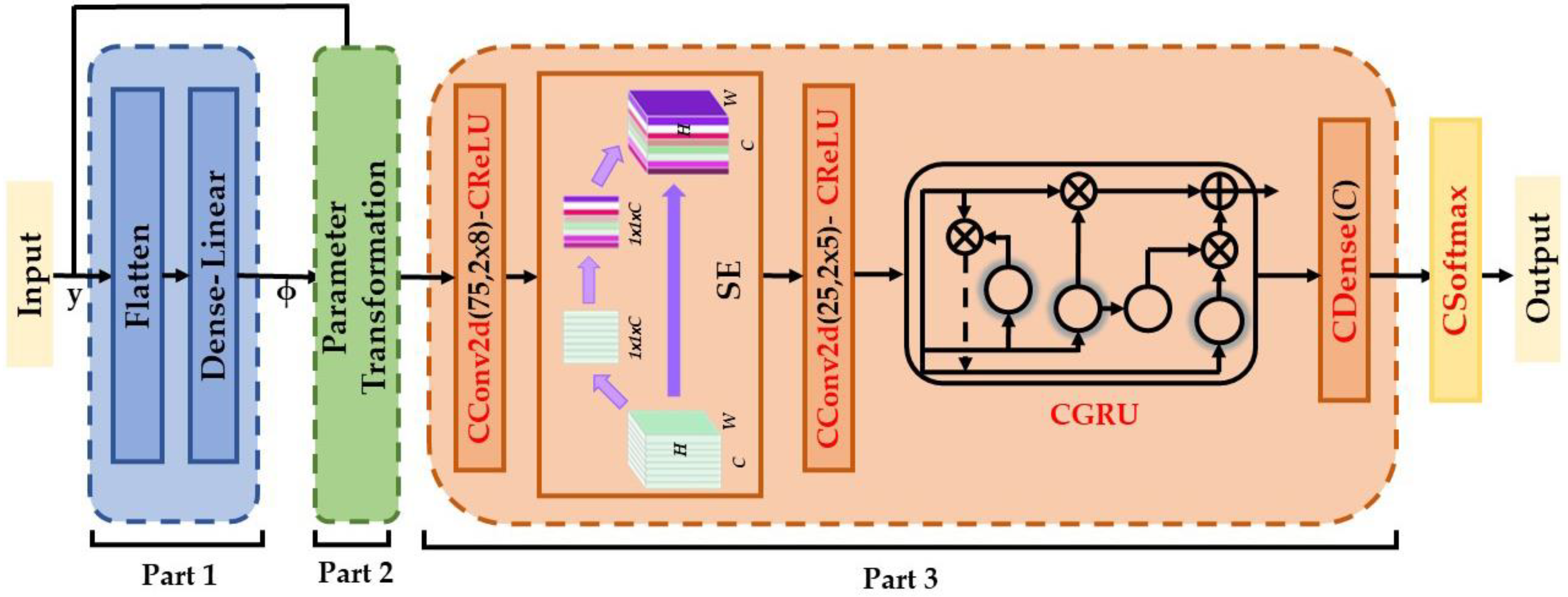
2.3. The Proposed Complex-Valued PET-CSGDNN Model

In order to realize the complex number calculation, based on the existing PET-CGDNN model [29], the network layers in the feature extraction, feature mapping, and classification parts are extended to the complex number framework. In order to dynamically modify the weights of various channels, SE block [30] which is a simple and lightweight channel attention method, is introduced in channel feature extraction, as shown in Figure 1. Part 1 can estimate the phase parameters of the input signal by co-training with the following model: The parameter transformation in Part 2 is a custom layer that uses the input signals and phase parameters to carry out an inverse parameter transformation with input signals and phase parameters. Part 3 consists of complex-valued CNN, complex-valued ReLU, complex-valued GRU, complex-valued DNN, SE block, and complex softmax, and its main function is to implement feature extraction and classification. Specifically, the first complex convolutional layer has 75 filters and a kernel size of 2 × 8 to extract the spatial features of the signal, while the second complex convolutional layer has 25 filters and a kernel size of 2 × 5 to further compress the extracted features of the signal. The subsequent complex-valued GRU layer extracts the temporal features of 128 units of signals. The SE block is added to learn the connections between different channels and dynamically adjust the weights of different channels so as to enhance the performance of the model. In the SE block, the fully connected channel drops by a factor of two. The structure of the SE module is depicted in Figure 1. Firstly, the spatial feature compression is performed on the feature map, and the global average pooling is realized in the spatial dimension to obtain the feature map of 1 × 1 × C. Then, the feature map with channel attention is obtained by fully connected layer learning, and its dimension is still 1 × 1 × C. Finally, the feature map with channel attention is output after the feature map of the original input and the feature map of the channel attention have both been multiplied by the weight coefficient channel by channel. Finally, the classification operation is performed by the complex dense layer with the same number of hidden units (C) as modulation schemes. Complex ReLU is used as the activation function in the first two convolutions, and complex softmax is used after the last dense layer.

3. Experiments

The proposed model is subjected to ablation tests in this section, along with a comparison to existing benchmark models. We will first introduce the datasets used in our experiments, the experimental conditions, and the evaluation methods. Then, we will introduce the experimental arrangement of the ablation experiment and the comparison experiment, as well as the parameter settings of each benchmark model in the experiment.

3.1. Datasets and Experimental Conditions

The open-source modulation classification datasets named RML2016.10a and RML2018.01a (as shown in

Table 1. AMC Open-source Dataset [31].

Dataset	Modulation Schemes	Sample Dimension	Dataset Size	SNR Range (dB)
RML2016.10a	11 classes (8PSK, BPSK, CPFSK, GFSK, PAM4, 16QAM, AM-DSB, AM-SSB, 64QAM, QPSK, WBFM)	128 × 2	220,000	−20:2:18
RML2018.01a	24 classes (OOK, 4ASK, 8ASK, BPSK, QPSK, 8PSK, 16PSK, 32PSK, 16APSK, 32APSK, 64APSK, 128APSK, 16QAM, 32QAM, 64QAM, 128QAM, 256QAM, AM-SSB-WC, AM-SSB-SC, AM-DSB-WC, AM-DSB-SC, FM, GMASK, OQPSK)	1024 × 2	2,555,904	−20:2:30

), simulated and generated by the GNU Radio software platform, were used for verification in the experiments [31]. The loss function is the cross-entropy loss function. The optimizer is Adam; the initial value of the learning rate is 0.001, and when the validation loss does not decrease in 10 epochs, it is multiplied by a coefficient of 0.5; the number of training rounds is 200; the trained model is saved with the highest average accuracy; and the other hyperparameters are the default values. The GPU used in the experiment was GeForce GTX 3090, the CPU was Intel (R) Xeon (R) Gold 6248R, the operating system was Win 10 Education Edition, and the deep learning framework was Pytorch1.11.0.

3.2. Evaluation Method

In this paper, we introduce accuracy to measure the performance of the generalization ability of the proposed model, as shown in Equation (14):

$$Accuracy=\frac{TP+TN}{TP+TN+FP+FN}$$

(14)

According to the results of the true and predicted values, the whole sample set can be separated into true positive (TP), false positive (FP), true negative (TN), and false negative (FN), so the accuracy is the ratio of all correctly categorized samples to the total number of samples.

Experiments were carried out on RML2016.10a and RML2018.01a. First of all, random sampling without replacement was used with assignment ratios of 6:2:2 and 3:4:4, respectively. Secondly, the training samples were trained, and the validation samples were used to verify the model after each round of training. Then, after 200 rounds of training, the model parameters with the highest recognition accuracy on the validation sample were selected as the final model parameters. Finally, the test sample was input into the final model to obtain the model recognition accuracy results.

3.3. Experiment Settings

Experiment 1 is the ablation experiment; the PET-CGDNN [29], CV-PET-CGDNN, and CV-PET-CSGDNN models are compared under the RML2016.10a and RML2018.01a data sets. Among them, CV-PET-CGDNN is the PET-CGDNN model extended to the complex-valued framework according to the method in Section 2.2, aiming to verify whether the proposed CV-PET-CGDNN is conducive to fully extracting features between in-phase and quadrature time series data and improving the recognition accuracy of modulation modes. CV-PET-CGDNN is the version of the CV-PET-CSGDNN model without an attention module, which is designed to verify the effectiveness of the attention module introduced in this model for the acquisition of channel relationship weights.

Experiment 2 is a comparison test. In order to verify the generalization and effectiveness of the CV-PET-CSGDNN model, key AMC models are selected to provide benchmark comparisons, including ResNet [2], CLDNN [32], MCLDNN [33], PET-CGDNN [29], and CV-ResNet [12]. ResNet, CLDNN, MCLDNN, and PET-CGDNN are RVNNs. CV-ResNet and CV-PET-CSGDNN are CVNNs. CLDNN, MCLDNN, PET-CGDNN, and CV-PET-CSGDNN are all hybrid models, and the network structure and parameter settings are shown in

Table 2. Structure of the compared network.

Model	ResNet	CLDNN	MCLDNN	PET-CGDNN
Input	I/Q	I/Q	I/Q, I and Q	I/Q
Convolution Layers	4	3	5	2
Kernel Size	3 × 1, 3 × 2, 3 × 1, 3 × 1	8 × 1	8 × 2, 7, 7, 8 × 1, 5 × 2	2 × 8, 1 × 5
Convolution Channels	256, 256, 80, 80	50 × 3	50 × 4	75, 25
LSTM Layers	0	1	1	0
LSTM Units	0	50 × 1	128 × 1	0
Dense	2 (128, C *)	1 (256, C *)	3 (128, 128, C *)	1 (C *)

* C is the number of modulation schemes.

and

Table 3. Structure of the complex-valued neural network.

Model	CV-ResNet	CV-PET-CSGDNN
Input	I/Q	I/Q
Complex Convolution	4	2
Kernel Size	3, 3, 3, 3	8, 5
Convolution Channels	64,64,20,20	75, 25
Complex-valued GRU	0	1 (128)
Complex-valued Dense	2 (128, C *)	1 (C *)

* C is the number of modulation schemes.

, respectively. Other details of benchmark models are displayed in

Table A2. Details of the benchmark models.

Abbreviations	Author	Details
ResNet	Liu et al. [32]	ResNet
CLDNN	Liu et al. [32]	CNN + LSTM
MCLDNN	Xu et al. [33]	CNN + LSTM (Multi-channel)
PET-CGGDNN	Zhang et al. [29]	CNN + GRU + DNN
CV-ResNet	Kim et al. [12]	Complex-valued CNN + Complex-valued DNN

.

4. Results and Discussions

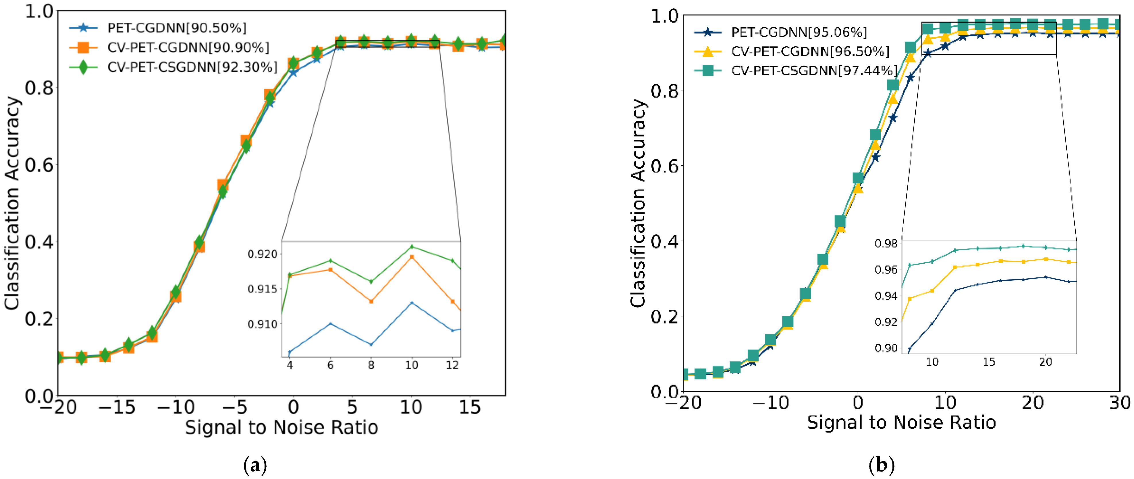
4.1. Ablation Experiments

Table 4. (Ablation Experiments) Average recognition accuracy of the models on different datasets (A: RML2016.10a, B: RML2018.01a).

	Dataset	A (6:2:2)	B (3:4:4)
Model
PET-CGDNN		60.60%	60.29%
CV-PET-CGDNN		60.90%	61.67%
CV-PET-CSGDNN		61.50%	62.89%

shows the average classification accuracy of the improved model CV-PET-CSGDNN proposed in this paper, the benchmark model PET-CGDNN, and the extended complex framework CV-PET-CGDNN model on different datasets. It can be seen from Table 4 that when the PET-CGDNN model is extended to the CV-PET-CGDNN for modulation classification on RML2016.10a and RML2018.01a, the average recognition accuracy is effectively improved by 0.30% and 1.38%, respectively. This shows that the expansion of the CVNN is very beneficial to the feature extraction of the relationship between I/Q channels and then improves the accuracy of modulation classification. When the model is extended from CV-PET-CGDNN to CV-PET-CSGDNN, the average recognition accuracy on different datasets are improved, which is 0.60% and 1.22%, respectively, indicating that the introduction of the attention mechanism module effectively learns the relationship between different channels and improves the performance of the model. Compared with the benchmark model PET-CGDNN on RML2016.10a and RML2018.01a, the average recognition accuracy of the CV-PET-CSGDNN model proposed in this paper is increased by 0.90% and 2.60%, respectively. Similarly, from the magnification area of Figure 2, we can see that the curve of CV-PET-CSGDNN is higher than the other two, indicating that the classification accuracy of CV-PET-CSGDNN is higher than that of the other two models.

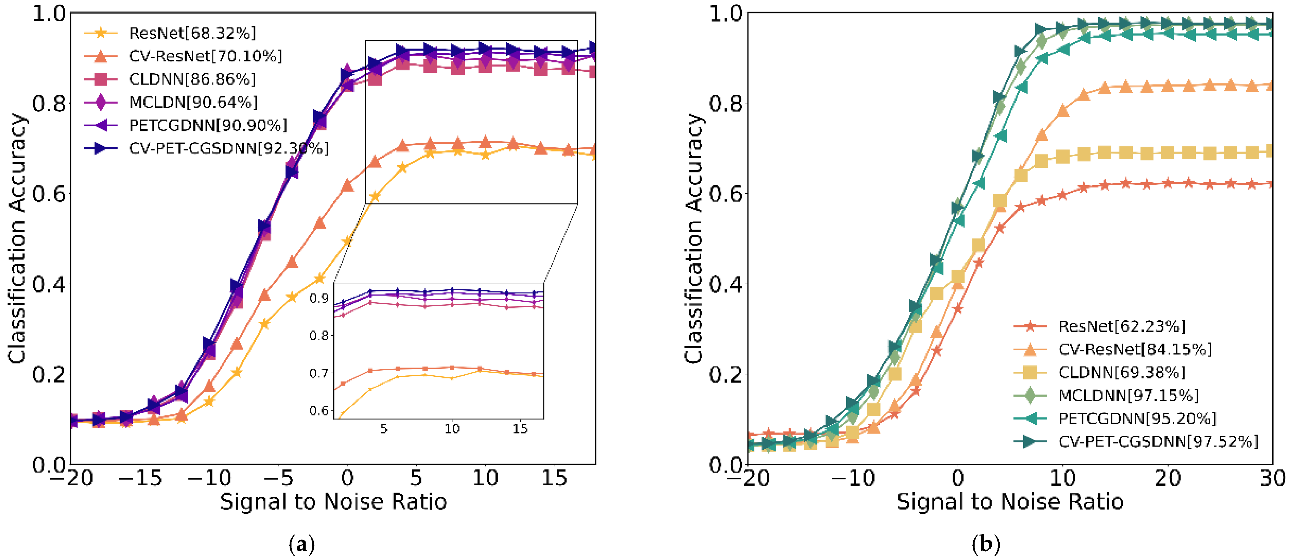
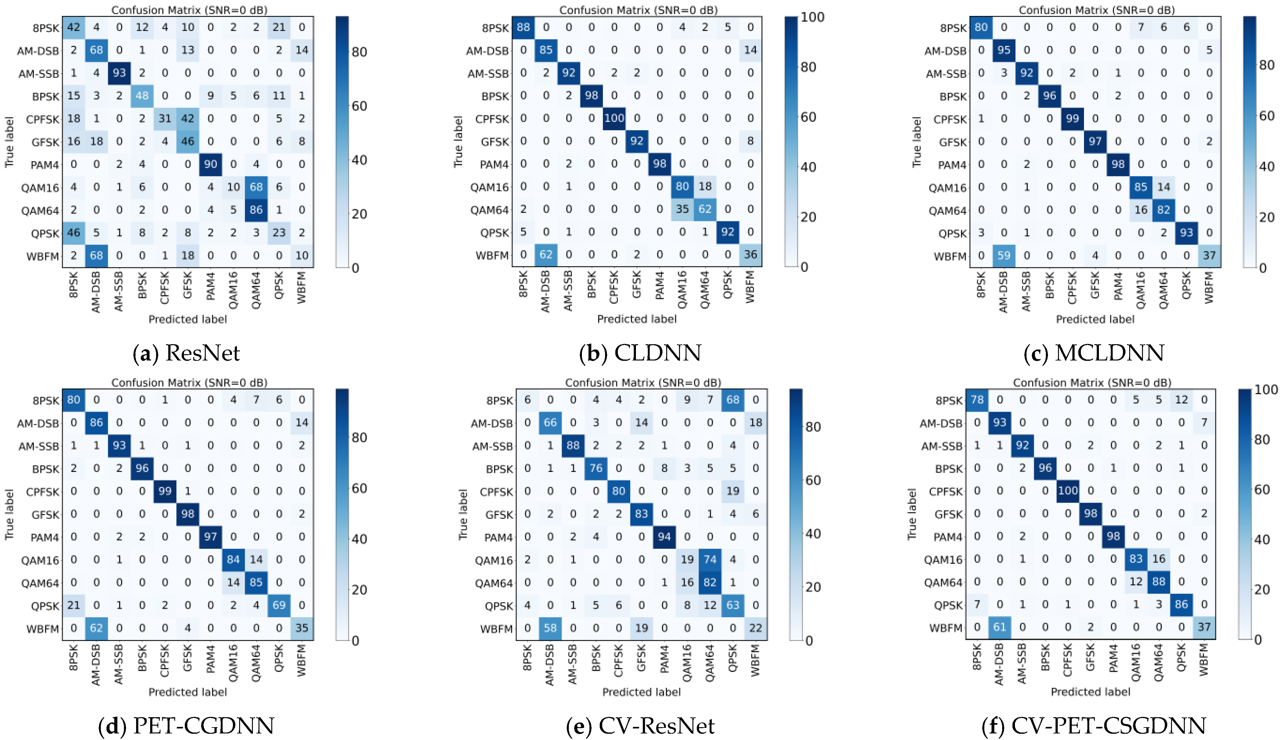
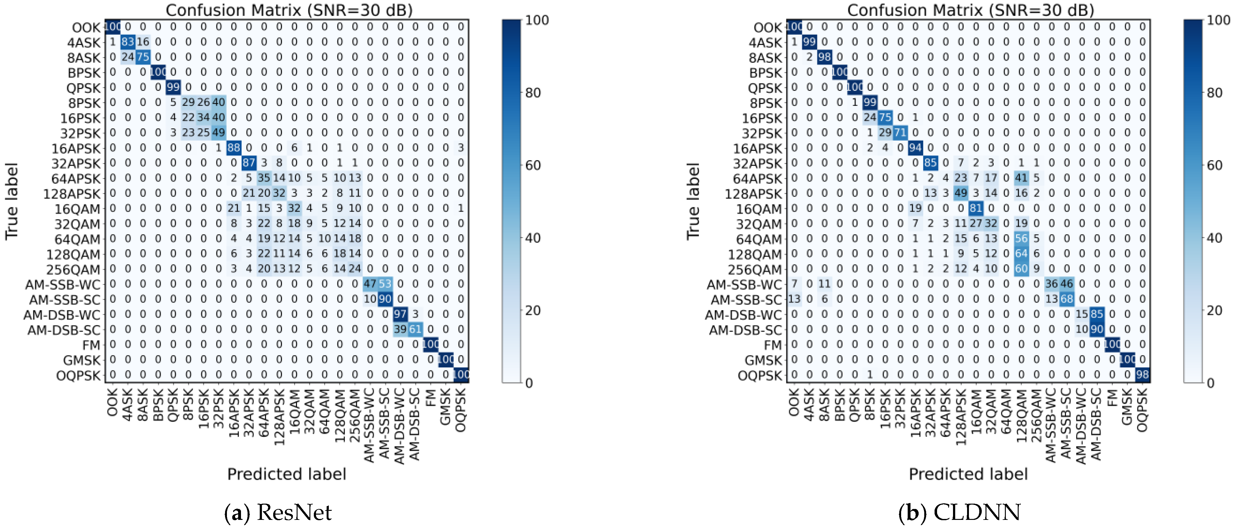
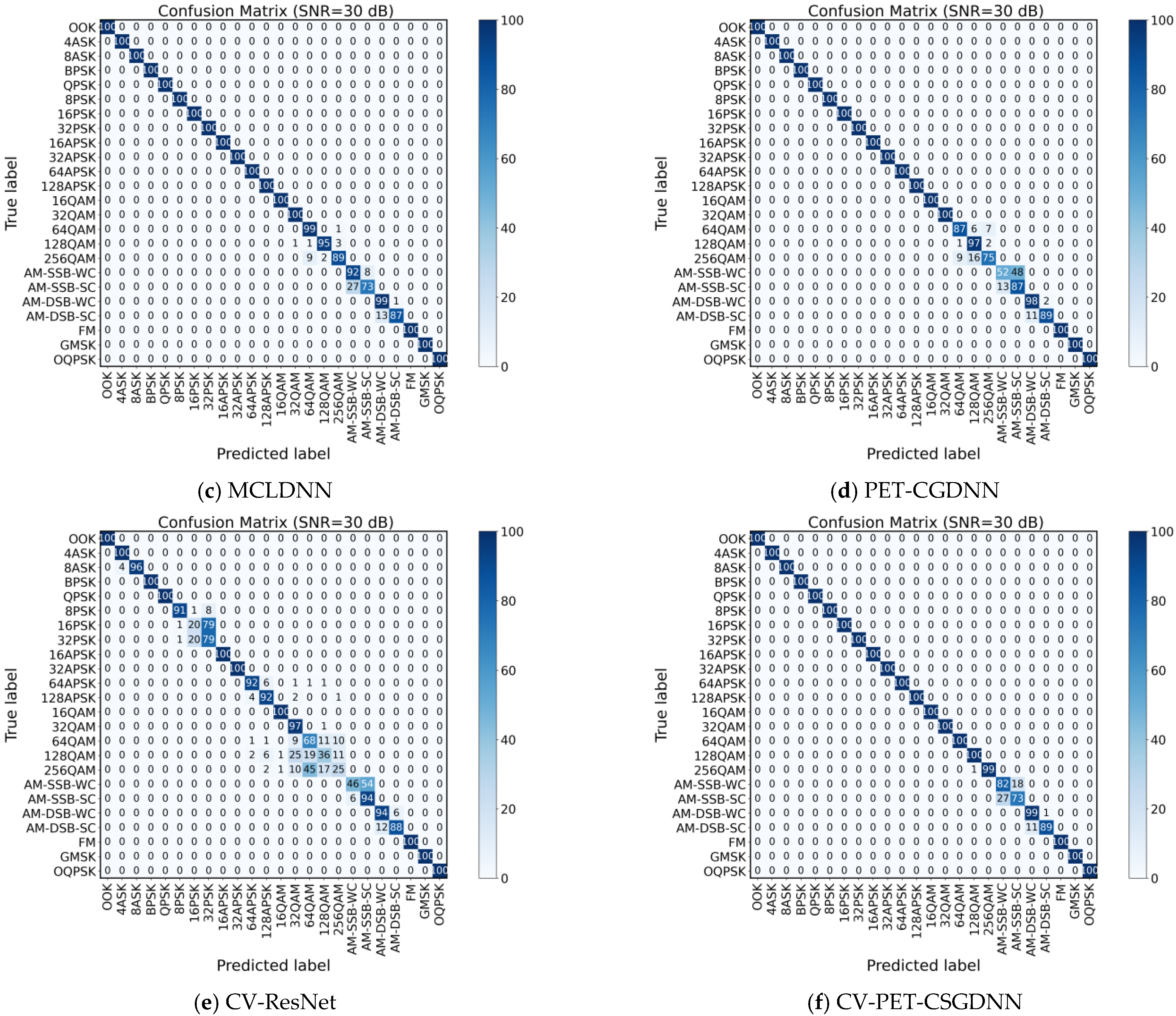
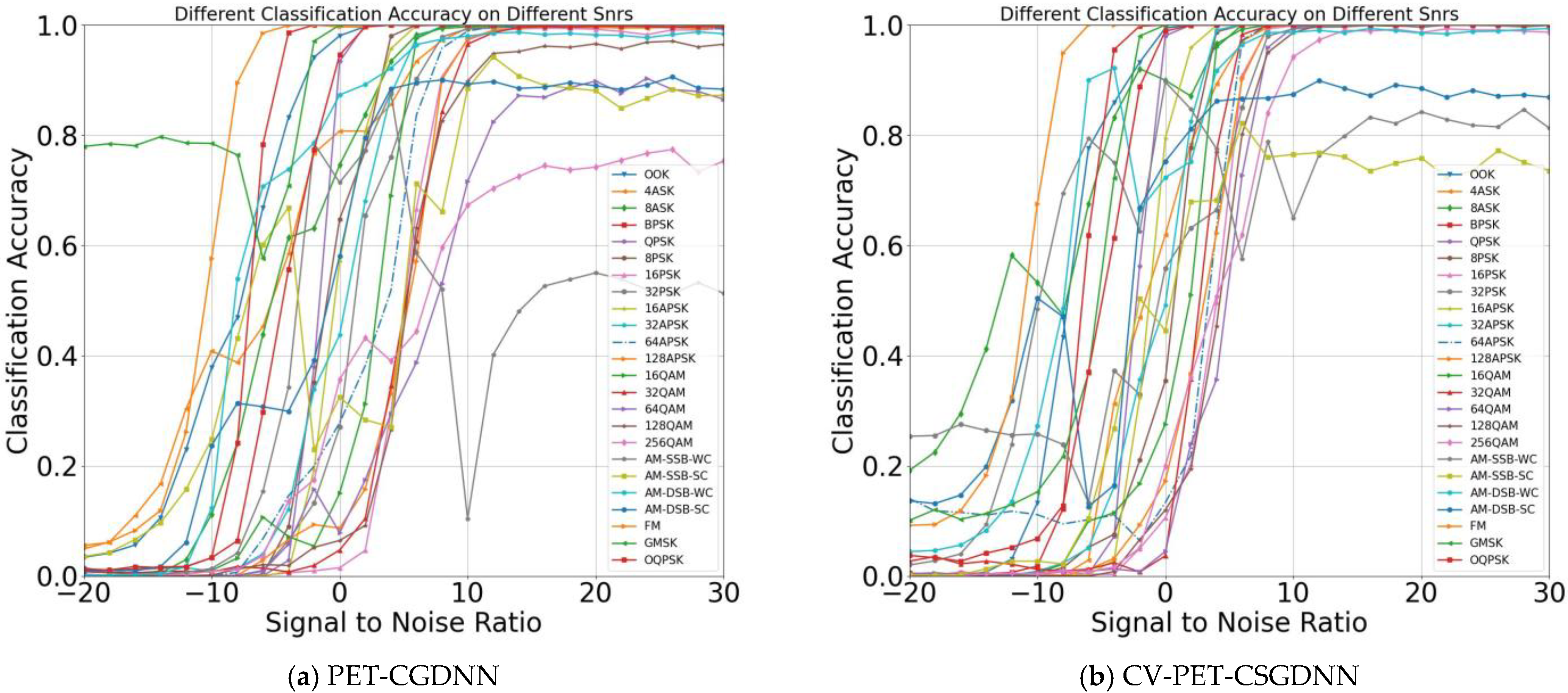
4.2. Comparative Experiments of Different Networks

Table 5. Model comparison on two datasets(A: RML2016.10a, B: RML2018.01a).

Model	Data- Sets	Capacity *	Training Time (Second /Epoch)	Test Time (ms/Sample)	Average Accuracy (All SNR)	Average Accuracy (≥0 dB)	Highest Accuracy
ResNet	A	3098 K	11.085	11.381	42.51%	65.89%	69.78%
	B	2660 K	431.620	12.211	39.55%	57.89%	62.23%
CLDNN	A	76 K	23.055	0.540	59.14%	87.22%	88.45%
	B	80 K	527.657	1.958	44.93%	64.85%	69.38%
MCLDNN	A	405 K	19.379	0.023	60.51%	89.37%	90.73%
	B	408 K	427.981	0.850	61.84%	90.86%	97.29%
PET-CGDNN	A	71 K	12.200	0.010	60.60%	89.80%	91.27%
	B	75 K	181.658	0.237	60.25%	87.80%	95.45%
CV-ResNet	A	364 K	11.980	0.010	46.27%	69.45%	71.45%
	B	2660 K	183.692	0.397	49.97%	74.95%	84.15%
CV-PET-CSGDNN	A	86 K	15.147	0.023	61.50%	90.90%	92.32%
	B	90 K	384.298	0.827	62.92%	91.67%	97.75%

* Capacity is the number of parameters.

shows the recognition accuracy of the proposed CV-PET-CSGDNN model and other models on different datasets. Table 5 shows that the average recognition accuracy of CV-PET-CSGDNN is the highest on RML2016.10a and RML2018.01a. Compared with CV-ResNet, which is also a CVNN, the average accuracy under all SNR is increased by 15.23% and 12.95%, respectively, and the parameters are reduced by 76.22% and 96.61%, respectively. Compared with the MCLDNN model with a good average recognition accuracy, the number of parameters in CV-PET-CSGDNN is reduced by 78.64% and 77.91%, respectively. Compared with the PET-CGDNN model, the average recognition accuracy under all SNR is increased by 0.69% and 2.14%, and the average recognition accuracy under SNR greater than 0 dB is increased by 0.81% and 2.77%.

Figure 3 shows the recognition accuracy of each model on RML2016.10a and RML2018.01a. As shown in Figure 3, the recognition accuracy of the proposed CV-PET-CSGDNN model performs the best compared to other models. In particular, when the SNR is 18 dB, the recognition accuracy of the model is 92.30% on RML2016.10a. When the SNR is 30 dB, the recognition accuracy of the model is 97.52% on RML2018.01a. Figure 4 shows the confusion matrix of the proposed CV-PET-CSGDNN and other benchmark models on RML2016.01a when the SNR is 0 dB. Figure 5 shows the confusion matrix of the proposed CV-PET-CSGDNN and other benchmark models on RML2018.10a when the SNR is 30 dB. In a confusion matrix plot, the color depth represents the intensity or density of the values in each cell. Therefore, the color depth means less misjudgment and high classification accuracy. According to Figure 4 and Figure 5, compared with benchmark models, the diagonal relationship of CV-PET-CSGDNN is more obvious, which indicates that its recognition effect is the best. As shown in Figure 5f, there are mainly misjudgments in the classification of two groups of modulation schemes: AM-DSB-WC and AM-DSB-SC, AM-SSB-WC and AM-SSB-SC, so that the average recognition cannot reach 100% when the SNR is 30 dB. For an amplitude modulation signal, only the amplitude of the carrier changes in proportion to the amplitude of the information signal [12]. In other words, a pure amplitude modulation signal only consists of a real part and no imaginary part. Therefore, it might be the main reason for the misjudgment of AM modulation signals in AMC models based on CVNNs. Such a situation also exists in other CVNNs [2]. There are also some misjudgments among similar modulation methods in RVNNs, so that the average recognition accuracy cannot reach 100% under high SNRs [2]. In addition, it is apparent that the proposed CV-PET-CSGDNN has a significant improvement in the misjudgment situation between 64QAM, 128QAM, and 256QAM compared with PET-CGDNN on RML2018.01a, as shown in Figure 5. Furthermore, the classification accuracy of PET-CGDNN and CV-PET-CSGDNN for each modulation scheme on RML2018.01a is displayed in Figure 6. The recognition accuracy of most modulation schemes improves, especially 64QAM, 128QAM, and 256QAM, which could also verify that the proposed CV-PET-CSGDNN can improve the accuracy of model recognition.

5. Conclusions

In this paper, a complex-valued hybrid neural network based on complex-valued CNN and complex-valued GRU is proposed, which can identify the original I/Q waveform of each modulated signal inherent to the coherence information of the signal, making full use of the intrinsic relationship between in-phase and quadrature time series data. Experiments show that the proposed model can robustly and efficiently identify the signal modulation from the original signal without any prior knowledge. Compared with ResNet, CLDNN, MCLDNN, PET-CGDNN, and CV-ResNet, our proposed CVNN achieves the highest average accuracy of 61.50% and 62.92%, respectively, for AMC with a relatively low number of parameters. In addition, the proposed CV-PET-CSGDNN has a significant improvement in the misjudgment situation between 64QAM, 128QAM, and 256QAM compared with PET-CGDNN on RML2018.01a. Therefore, our proposed CVNN has superior performance, which has the potential to be applied in scenarios with limited computing power and storage space and can be applied to satellite on-orbit applications in the future. And future research could focus on addressing the misjudgment issue of AM modulation signals in AMC models that rely on CVNNs. Additionally, new techniques for data preprocessing or augmentation could be explored to improve the robustness of the model to variations in the input signals.

References

1. Huynh-The, T.; Pham, Q.-V.; Nguyen, T.-V.; Nguyen, T.T.; Ruby, R.; Zeng, M.; Kim, D.-S. Automatic Modulation Classification: A Deep Architecture Survey. IEEE Access 2021, 9, 142950–142971. [Google Scholar] [CrossRef]
2. Zhang, F.; Luo, C.; Xu, J.; Luo, Y.; Zheng, F.-C. Deep learning based automatic modulation recognition: Models, datasets, and challenges. Digit. Signal Process. 2022, 129, 10365. [Google Scholar] [CrossRef]
3. Hong, D.; Zhang, Z.; Xu, X. IEEE Automatic Modulation Classification using Recurrent Neural Networks. In Proceedings of the 3rd IEEE International Conference on Computer and Communications (ICCC), Chengdu, China, 13–16 December 2017. [Google Scholar]
4. Li, L.; Dong, Z.; Zhu, Z.; Jiang, Q. Deep-Learning Hopping Capture Model for Automatic Modulation Classification of Wireless Communication Signals. IEEE Trans. Aerosp. Electron. Syst. 2023, 59, 772–783. [Google Scholar] [CrossRef]
5. Li, W.; Xie, W.; Wang, Z. Complex-Valued Densely Connected Convolutional Networks. In Data Science; Zeng, J., Jing, W., Song, X., Lu, Z., Eds.; Springer: Berlin/Heidelberg, Germany; Singapore, 2020; pp. 299–309. [Google Scholar]
6. Zeng, Z.; Sun, J.; Han, Z.; Hong, W. SAR Automatic Target Recognition Method Based on Multi-Stream Complex-Valued Networks. IEEE Trans. Geosci. Remote Sens. 2022, 60, 5228618. [Google Scholar] [CrossRef]
7. Tu, Y.; Lin, Y.; Hou, C.; Mao, S. Complex-Valued Networks for Automatic Modulation Classification. IEEE Trans. Veh. Technol. 2020, 69, 10085–10089. [Google Scholar] [CrossRef]
8. Zhang, F.; Luo, C.; Xu, J.; Luo, Y. An Autoencoder-Based I/Q Channel Interaction Enhancement Method for Automatic Modulation Recognition. IEEE Trans. Veh. Technol. 2023, 72, 9620–9625. [Google Scholar] [CrossRef]
9. Bassey, J.; Li, X.; Qian, L. A Survey of Complex-Valued Neural Networks. arXiv 2021, arXiv:2101.12249v1. [Google Scholar]
10. Hirose, A. Complex-Valued Neural Networks (Studies in Computational Intelligence); Springer: Berlin/Heidelberg, Germany, 2012. [Google Scholar]
11. Hirose, A. Complex-valued neural networks: The merits and their origins. In 2009 International Joint Conference on Neural Networks; IEEE: Atlanta, GA, USA, 2009; pp. 1237–1244. [Google Scholar]
12. Kim, S.; Yang, H.-Y.; Kim, D. Fully Complex Deep Learning Classifiers for Signal Modulation Recognition in Non-Cooperative Environment. IEEE Access 2022, 10, 20295–20311. [Google Scholar] [CrossRef]
13. Hirose, A.; Yoshida, S. Comparison of Complex- and Real-Valued Feedforward Neural Networks in Their Generalization Ability. In Neural Information Processing; Springer: Berlin/Heidelberg, Germany, 2011; pp. 526–531. [Google Scholar]
14. Lee, C.; Hasegawa, H.; Gao, S. Complex-Valued Neural Networks: A Comprehensive Survey. IEEE/CAA J. Autom. Sin. 2022, 9, 1406–1426. [Google Scholar] [CrossRef]
15. Hirose, A. Continuous complex-valued back-propagation learning. Electron. Lett. 1992, 28, 185. [Google Scholar] [CrossRef]
16. Hirose, A. Dynamics of fully complex-valued neural networks. Electron. Lett. 1992, 28, 1492. [Google Scholar] [CrossRef]
17. Hirose, A. Complex-valued neural networks: Distinctive features. Stud. Comput. Intell. 2006, 400, 17–56. [Google Scholar]
18. Hirose, A. Recent Progress in Applications of Complex-Valued Neural Networks. In Proceedings of the International Conference on Artifical Intelligence & Soft Computing, Zakopane, Poland, 13–17 June 2010. [Google Scholar]
19. Hirose, A.; Yoshida, S. Generalization Characteristics of Complex-Valued Feedforward Neural Networks in Relation to Signal Coherence. IEEE Trans. Neural Netw. Learn. Syst. 2012, 23, 541–551. [Google Scholar] [CrossRef]
20. Nitta, T. On the critical points of the complex-valued neural network. In Proceedings of the 9th International Conference on Neural Information Processing, 2002, ICONIP ’02, Singapore, 18–22 November 2002. [Google Scholar]
21. Arjovsky, M.; Shah, A.; Bengio, Y. Unitary Evolution Recurrent Neural Networks. In Proceedings of the 33rd International Conference on Machine Learning, New York, NY, USA, 19–24 June 2016; p. 4. [Google Scholar]
22. Danihelka, I.; Wayne, G.; Uria, B.; Kalchbrenner, N.; Graves, A. Associative Long Short-Term Memory. In Proceedings of the 33rd International Conference on Machine Learning, New York, NY, USA, 20–22 June 2016; p. 48. [Google Scholar]
23. Wisdom, S.; Powers, T.; Hershey, J.R.; Le Roux, J.; Atlas, L. Full-Capacity Unitary Recurrent Neural Networks. In Proceedings of the 30th Conference on Neural Information Processing Systems (NIPS), Barcelona, Spain, 9 December 2016; p. 29. [Google Scholar]
24. Trabelsi, C.; Bilaniuk, O.; Zhang, Y.; Serdyuk, D.; Subramanian, S.; Santos, J.; Mehri, S.; Rostamzadeh, N.; Bengio, Y.; Pal, C. Deep Complex Networks. In Proceedings of the ICLR 2018, Vancouver, BC, Canada, 30 April–3 May 2018. [Google Scholar]
25. Marseet, A. Application of Convolutional Neural Network Framework on Generalized Spatial Modulation for Next Generation Wireless Networks. Graduate Thesis, Rochester Institute of Technology, Rochester, NY, USA, April 2018. [Google Scholar]
26. Chang, Z.; Wang, Y.; Li, H.; Wang, Z. IEEE Complex CNN-Based Equalization for Communication Signal. In Proceedings of the 4th IEEE International Conference on Signal and Image Processing (ICSIP), SE University, Wuxi, China, 19–21 July 2019. [Google Scholar]
27. Krzyston, J.; Bhattacharjea, R.; Stark, A. Complex-Valued Convolutions for Modulation Recognition using Deep Learning. In Proceedings of the 2020 IEEE International Conference on Communications Workshops (ICC Workshops), Dublin, Ireland, 7–11 June 2020; pp. 1–6. [Google Scholar]
28. Xu, J.; Wu, C.; Ying, S.; Li, H. The Performance Analysis of Complex-Valued Neural Network in Radio Signal Recognition. IEEE Access 2022, 10, 48708–48718. [Google Scholar] [CrossRef]
29. Zhang, F.; Luo, C.; Xu, J.; Luo, Y. An Efficient Deep Learning Model for Automatic Modulation Recognition Based on Parameter Estimation and Transformation. IEEE Commun. Lett. 2021, 25, 3287–3290. [Google Scholar] [CrossRef]
30. Hu, J.; Shen, L.; Albanie, S.; Sun, G.; Wu, E. Squeeze-and-Excitation Networks. arXiv 2019, arXiv:1709.01507. [Google Scholar]
31. O’Shea, T.J.; Roy, T.; Clancy, T.C. Over-the-Air Deep Learning Based Radio Signal Classification. IEEE J. Sel. Top. Signal Process. 2018, 12, 168–179. [Google Scholar] [CrossRef]
32. Liu, X.; Yang, D.; El Gamal, A. Deep Neural Network Architectures for Modulation Classification. In Conference Record of the Asilomar Conference on Signals Systems and Computers, Proceedings of the 51st IEEE Asilomar Conference on Signals, Systems, and Computers, Pacific Grove, CA, USA, 29 October–1 November 2017; IEEE: Atlanta, GA, USA, 2017; pp. 915–919. [Google Scholar]
33. Xu, J.; Luo, C.; Parr, G.; Luo, Y. A Spatiotemporal Multi-Channel Learning Framework for Automatic Modulation Recognition. IEEE Wirel. Commun. Lett. 2020, 9, 1629–1632. [Google Scholar] [CrossRef]
Figure 1. The structure of the proposed CV-PET-CSGDNN.
Electronics 12 04380 g001
Figure 2. Classification accuracy of different networks on RML2016.10a (a) and RML2018.01a (b). It is noted that “[%]” represents the average classification performance when the SNR is the highest.
Electronics 12 04380 g002
Figure 3. Classification accuracy of different networks on RML2016.10a (a) and RML2018.01a (b) It is noted that “[%]” represents the average classification performance when the SNR is the highest.
Electronics 12 04380 g003
Figure 4. Confusion matrices of the proposed and benchmark models on RML2016.01a when the SNR is 0 dB.
Electronics 12 04380 g004
Figure 5. Confusion matrices of the proposed and benchmark models on RML2018.10a when the SNR is 30 dB.
Electronics 12 04380 g005aElectronics 12 04380 g005b
Figure 6. Classification accuracy for each modulation scheme on RML2018.01a.
Electronics 12 04380 g006