Abstract
This paper explores the impact of gravity disturbances on INS accuracy and presents a method for real-time compensation during the navigation process. By utilizing data from the precise gravity model, EGM2008, a novel approach to compensate for the DOV in real time on the INS’s built-in NPU was introduced. This method predicts gravity disturbances while traveling for platforms on both land and water, utilizing the MLP technique. To predict these gravity disturbances, four distinct MLP models, MLP1~MLP4, were designed and their supervised learning results were compared using HMSE and RMSE. This comparative analysis allowed us to identify that the MLP4 model exhibited the best performance. In order to validate the proposed method, MLP4 was implemented inside the NPU and the measured execution time was 1.041 ms. The field test was conducted with real-time execution of the MLP4 model on the NPU of the INS. The results of this field test clearly demonstrated the effectiveness of the proposed approach in enhancing position accuracy. Over the course of a 2 h field test, it was evident that employing the proposed method improved position accuracy by a notable 27%.
1. Introduction
The Inertial Navigation System (INS) is an autonomous system capable of continuously determining a platform’s attitude, speed, and position using its built-in gyroscope and accelerometer [1,2]. This self-contained feature makes the INS impervious to external interference, rendering it invaluable in both military and civilian applications such as missile navigation and civil aircraft. However, the INS, particularly in the case of the dead reckoning approach, is susceptible to accumulating errors stemming from its own inertial sensor inaccuracies. Among these error sources, gyroscope and accelerometer drift bias emerge as significant contributors to INS inaccuracies. Substantial efforts have been invested in reducing the magnitude of these biases. On the one hand, advanced technologies like cold atom interferometry have been employed to enhance the precision of inertial sensors [3]. On the other hand, system-level compensation methods, such as rotational modulation, have significantly improved INS performance [4]. As INS performance has improved, previously overlooked error sources have come to the forefront, with gravity disturbances being one of the key factors limiting the further enhancement of INS accuracy [5].
Typically, the INS has used a value known as “normal gravity” to compensate for gravitational acceleration. This normal gravity is always perpendicular to the Earth’s ellipsoid, resulting in a horizontal component of ‘0’ and only a vertical component. The value can be computed using the Taylor series expansion of the Somigliana formula. The difference between normal gravity and actual Earth gravity is termed gravity disturbance, encompassing the gravity anomaly (magnitude of the difference between normal and actual gravity) and the horizontal gravity disturbance known as the Deflection Of the Vertical (DOV), which represents the angular deviation from normal gravity to Earth gravity. In error analysis of the INS, the DOV primarily impacts initial alignment and velocity calculation accuracy. Several studies, including those by Kwon and Jekeli [4], Jekeli [6], and Jekeli et al. [7], have explored the performance enhancement achieved through gravity compensation in error-free INS.
Hanson [8] investigated why DOV compensation is not universally applied in initial alignment and found a correlation between uncompensated accelerometer drift bias and the DOV. However, the conclusions in ref. [8] were qualitative, and the compensation procedure presented was specific to certain cases. George [9] introduced LN-93E, a military-standard ring laser inertial navigation device that improved performance through DOV compensation during alignment. It is worth noting that in prior studies, DOV compensation values were preloaded before alignment, relying on precalculated or measured values along the route rather than real-time calculations. Determining high-quality DOV compensation values over a large area requires significant computational resources, limiting DOV compensation to initial alignment in practice.
In [10], gravity disturbance compensation for the INS using measured gravity data was studied. The gravity disturbance was first predicted based on measured gravity data and compensated for in the INS error equations to restrain position error propagation. In [11], an artificial neural network called Extreme Learning Machine (ELM) was applied to compensate for gravity disturbances in real time with high precision, providing gravity and DOV values.
Recently, there has been increasing interest in employing high-resolution global gravity field models to compensate for gravity disturbances in the INS. Many such models are based on Spherical Harmonic Models (SHMs), with Earth Gravity Model 2008 (EGM2008) being a prominent example, featuring a maximum spherical degree and order of 2160. Studies [12,13,14,15,16] have investigated how SHMs, particularly EGM2008, can enhance INS performance. However, much of this work focused on simplifying SHMs for real-time applications due to limited computing power, especially in onboard INS computers. For instance, Wang et al. [13] assessed the feasibility and accuracy of a modified SHM for real-time INS applications, while Wang et al. [14] proposed a simplified 2D second-order polynomial model derived from an SHM. Wu et al. [15] explored the effective minimum update rate of gravity using an SHM for marine and airborne INS. In research [16], DOV compensation was investigated using EGM2008 for both initial alignment and navigation solution calculation, with the concluding that compensating for the DOV only during navigation solution calculation is most desirable. Wide research into gravity disturbance compensation, particularly for initial alignment and INS navigation computation, has been continuing.
Through many research results referenced in this paper, it has been proven that the position error of the INS is reduced by compensating for the DOV. However, the INS must provide real-time data on position, velocity, and attitude. Therefore, compensating for the DOV in real time must occur during the process of navigation computation inside the INS. However, it is difficult to find satisfactory research results about real-time DOV compensation in previous studies. Nevertheless, notable research results were found in the literature [11,14], but these also had certain issues. The research in [11] did not present the training results for the ELM and computation time in the INS’s embedded computer, which can vary based on the network size and computing environment. In paper [14] presented a short calculation time and high DOV prediction accuracy, but this required an external high-performance computer outside the INS to calculate the DOV and generate polynomial coefficients.
Considering this, we will discuss an MLP-based DOV compensation technique that can be executed in real time on the embedded Navigation Processing Unit (NPU) built into the INS. The key point covered in this study is to ensure that the designed MLP model can be executed in real time on the INS’s NPU. Therefore, the goal of this paper is to design an MLP network model that can accurately predict the DOV calculated in real time on the NPU and prove its performance through field tests. To achieve this, gravity disturbances will be calculated using the 2160th order EGM2008 SHM to generate the training data for MLP.
Afterwards, four MLP models will be designed that meet the required computational complexity, trained, and their final validation errors will be used to select the optimal model. The weights and biases of the trained network model will be transferred to the NPU for DOV computation, and the execution time will be measured, proving the feasibility of real-time DOV compensation inside the NPU. Furthermore, field tests will be performed to show that the real-time MLP compensation technique can actually improve the position accuracy of the INS.
To achieve this goal, the paper is organized as follows: the involved reference frames in the INS and gravity disturbance calculation using an SHM are established in Section 2. In Section 3, an analysis of the relationship between attitude errors in the initial alignment of the INS and gravity disturbance is performed to understand the reasons for compensating for gravity disturbances. In Section 4, the theory and framework of the MLP-based real-time gravity disturbance prediction method are described and the results of field tests are presented. Finally, conclusions are drawn in Section 5.
2. Reference Frames and Definition of Gravity Disturbance
2.1. Reference Frames
In the context of the INS, it is essential to define parameters within specific reference frames, as shown in Figure 1. Additionally, vectors initially expressed in one frame often need to be transformed into another. Hence, this section explores the coordinate frames employed in deriving the INS [5].
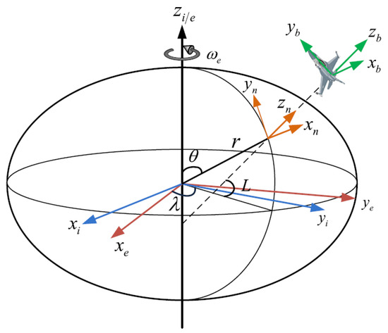
Figure 1.
The definition of reference frames.
- Earth-Centered Inertial Frame ‘e’: The Earth-Centered Inertial (ECI) frame is at the center of the Earth. Its z-axis aligns with the direction of the North Pole, the x-axis extends toward the mean vernal equinox, and the y-axis forms a right-handed orthogonal frame to complete the orientation. Importantly, the ECI frame remains nonrotating in relation to distant galaxies. Consequently, the outputs of both the gyroscope and accelerometer are referenced relative to this fixed ECI frame.
- Earth-Centered Earth-Fixed Frame ‘e’: The origin of this coordinate frame is located at the center of the Earth. The z-axis extends in the direction of the North Pole, the x-axis aligns with the Greenwich meridian, and the y-axis completes a right-handed orthogonal frame. This coordinate frame rotates along with the Earth at a constant rate, denoted . represents the angular velocity of the Earth’s rotation.
- Body coordinate frame with Right-Forward-Up definition ‘b’: This frame is defined based on the input axis of the inertial sensor, mounted on the platform, and points to the right-forward-up of the platform.
- Navigation coordinate frame with East-North Up definition ‘n’: This frame is the local geodetic coordinate frame with its origin at the vehicle’s position. Its x, y, and z-axis point towards east, north, and up, respectively. The INS calculation is conducted in the navigation frame. Therefore, all vectors should be transformed into this frame, represented by geodetic latitude (), longitude (), and height (). The position vector in the Earth-Centered Earth-Fixed (ECEF) frame can be obtained according to the geodetic values as:
The previously mentioned reference frames are commonly utilized in the INS. Commonly, spherical harmonic expansion is used to represent the Earth’s gravitational field with high fidelity [14]. To use high-precision gravity data effectively, we need to establish the connection between Cartesian coordinates and spherical coordinates. In the spherical coordinate system, the position vector is represented as with representing the spherical polar angle, as illustrated in Figure 1. As Figure 1 suggests, we can define the relationship between Cartesian coordinates and spherical coordinates using Equation (3). By combining Equations (1) and (3), we can determine the position in the spherical coordinate system based on the geodetic position .
2.2. Gravity Disturbances and Deflection of Vertical
Figure 2 illustrates the concept of gravity disturbance. According to potential theory, the gravity vector corresponds to the perpendicular line of an equipotential surface of gravity. The Earth’s equipotential surface of gravity is highly complicated, and for practical purpose, we often approximate it using a reference ellipsoid model like WGS-84. As depicted in Figure 2, g represents the Earth’s gravity vector at point P and denotes the normal gravity vector at the same point. The gravity disturbance vector, in turn, is the difference between the Earth’s gravity vector and the normal gravity vector. The disparity in their magnitudes defines the gravity disturbance, while the difference in their directions gives rise to the DOV. Owing to the DOV, there exist certain projection components of the Earth’s gravity vector within the horizontal plan, which are referred to as the horizontal gravity disturbance.
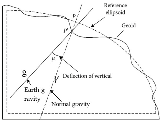
Figure 2.
Description of gravity disturbance vector and normal gravity.
The gravity disturbance, , is defined as the difference between Earth’s true gravity, , and the normal gravity, , and can be expressed as:
where the eastern and northern components of the gravity disturbance are denoted by and . is called the normal gravity perturbation or gravity anomaly. And is the norm of the normal gravity vector. The superscript n means that these vectors are projected onto n-coordinate frames.
For the DOV, the northern and eastern angular components are represented by and , respectively, as shown in Figure 3. The relationship between horizontal gravity disturbance and the DOV is as follows [7]:
where is the magnitude of vertical gravity and can be calculated directly using the EGM2008 model.
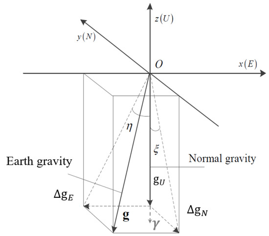
Figure 3.
The definitions of deflection of vertical, normal gravity, and Earth gravity.
For a global target, the magnitude of the DOV component can reach up to 100 arcsec (1 arcsec = 1º/3600), corresponding to 500 mGal (1 mGal = 10−5 m/s2) in terms of accelerometer bias. This value is significantly larger than the bias value of 10 mGal, typical for high-precision accelerometers [6]. By incorporating Equation (5) into Equation (4), the gravity disturbance can be expressed as:
where the horizontal gravity disturbance can be calculated through a spherical harmonic model (SHM) of the Earth’s gravity field, as follows [3,17]:
where G is the gravitational constant, M is the mass of the Earth, is the length of the principal axis of the reference ellipsoid, is the radial distance from the calculated point to the center of the reference ellipsoid, and is the latitude defined in the spherical coordinate system. is the longitude of the calculated point; n and m are the degree and order of the SHM. and are the coefficients of the SHM. is the highest degree used in the SHM calculation; and is the fully normalized Legendre function of degree n and order m.
3. The Effect of DOV on Initial Alignment Attitude Errors in INS
In this chapter, we will analyze the impact of the DOV on the INS initial alignment procedure.
3.1. Kinematic Equations of INS
The attitude kinematics equation using DCM parameterization is defined as:
where is the angular velocity of the body relative to the navigation frame and is defined as:
where is the angular velocity of the body relative to the inertial frame and is measured by the gyroscope, and is the angular velocity of the Earth’s rotation and is defined as:
Also, is the angular rate of the navigation frame relative to the ECI frame caused by the linear motion of the object on the ellipsoidal surface. is given as:
where and are the meridian and transverse radius of the curvature of the ellipsoid, respectively. and are the eastern and northern components of velocity, respectively. The velocity kinematics equation of the navigation frame is defined as:
where is the specific force measured by the accelerometer. is the gravity vector, which can be the high-precision gravity calculated through the EGM2008 gravity model or the normal gravity model.
The position kinematics equations are as follows:
where is the vertical component of the INS’s velocity represented in the n-frame.
3.2. Error Equations
Typically, the initial alignment is performed in a stationary state, so the actual velocity of the INS is nearly zero. In this case, the non-zero velocity output of the INS represents the velocity error, and the Kalman filter (KF) can be used to estimate the corresponding error of the INS. The KF for initial alignment is built based on the error equations of the INS.
If the attitude error and velocity error are expressed as and , respectively, the corresponding linear error equation is given in [5], as follows:
where is the attitude error vector, is the east component of the attitude error vector, is the north component, and is the vertical component. is the velocity error vector, is the noise of the accelerometer, is the direction cosine matrix (DCM) from the b-frame to the n-frame, and is the skew symmetric matrix of the specific force of the n-frame, as shown in Equation (17):
where is the eastern component of the specific force, is the north component, and is the upper component.
Next, we will focus on the influence of on the INS error equation. Gravity disturbance is defined as the difference between true gravity and normal gravity in the INS calculation. In practice, the true value of gravity or absolutely exact gravity cannot be obtained, so normal gravity is traditionally used in the INS. We can assume that the gravity obtained by an ultra-precision gravity model like EGM2008 can be regarded as the true gravity, and the disturbance is denoted as:
It is evident that gravity disturbances directly affect velocity error propagation and have an impact on attitude and position errors through error coupling. When a high-accuracy gravity model can be obtained, gravity disturbances should be considered as one of the sources of INS error and compensated for. However, the effect of is influenced by the error source . If the magnitudes of these two error sources are similar and the signs are opposite, their effects on velocity error can cancel each other out. In this case, using a high-precision gravity model for the INS may result in higher performance compared to using a normal gravity model. However, it is important to note that the sign of , especially in dynamic cases, cannot be determined in advance, as it is time-varying under the influence of . Therefore, in such cases, it is still advisable to conservatively use a normal gravity model.
If the accelerometer drift bias is pre-calibrated or modulated through rotation, gravity disturbances become the dominant error source in the velocity error equation. In this scenario, they must be compensated for. Conversely, if the accelerometer drift bias is much larger than the gravity disturbance, the compensation performance is expected to be reduced.
3.3. Initial Alignment Attitude Error Analysis by DOV
Assuming an initial alignment process in a stationary state, we can derive the velocity errors of the INS. The errors , , and can be determined through calculations and treated as parameters. Therefore, by rearranging Equation (16), we obtain the following Equation:
where is a linear combination of known parameters and converges to ‘0’ since we assume a stationary state. Expanding Equation (19), we can express the east and north components as follows:
where and represent the east and north components of , respectively. and are the east and north components of the accelerometer drift bias in n-frame, respectively.
In this paper, we focus on analyzing only the east and north components as we separate the vertical and horizontal channels. We assume that the platform is in a stationary state with a negligible inclination angle. Therefore, we establish , and . Substituting these into Equations (20) and (21), we can express the east and north components of the attitude error as follows:
by combining Equation (5), Equations (22) and (23) can be rewritten as:
where can be divided into two parts. is independent of the DOV and the random bias of the northern accelerometer component acts as a major error factor. Residual means the eastern component of the attitude estimation error due to the DOV is equal to . It can be divided into and in the same way for . Similarly, is independent of the DOV and the random bias of the accelerometer to the eastern accelerometer component is a major error factor, while is the north component of the attitude estimation error due to the DOV, and has a negative relationship with .
The attitude error transition function of the INS in the n-frame is expressed in Equation (15). Since in Equation (15), and are relatively small compared to the other error terms, we can reasonably ignore their effects in the following analysis.
Expanding Equation (15), we can express the corresponding east, north, and vertical components as follows:
where , and denote the east, north and vertical components of gyro random bias represented in the n-frame. and denote the north and vertical components of .
From Equations (26)–(28), it is evident that , and are coupled to each other. Therefore, if the DOV causes an error in the inclination angle of the platform, it can also affect the estimation of the azimuth angle. By rearranging Equation (26) for , we obtain:
The azimuth error can be calculated from Equation (29). Since the platform’s velocity is close to ‘0’ during initial alignment, we can assume and can be expressed as follows:
Therefore, Equation (29) can be expressed as:
Combining Equations (24), (31), and (26), we can rewrite Equation (32) as:
From Equation (33), we can see that has a negative correlation with and . Additionally, it can also be influenced by the magnitude of rather than by .
4. Theory and Framework of the MLP-Based Real-Time DOV Compensation in INS
With the current increase in computing power and widespread adoption of GPUs, neural network technology has demonstrated its value across a wide range of fields, consistently delivering exceptional results. It has become one of the most utilized tools for tackling complex problems that traditionally required intricate mathematical models. Notably, it has shown promise in addressing real-time prediction of the Degree of Vertical (DOV) in a high-order precise gravity model.
Artificial neural networks, often referred to simply as neural networks, draw loose inspiration from biological neural networks found in animal brains. A fundamental characteristic shared by both artificial and biological neural networks is their ability to learn tasks from examples rather than relying on explicit programming. Neural networks consist of interconnected nodes known as artificial neurons, which model the neurons present in biological systems. These nodes, connected via synapses, transmit or inhibit information in response to specific activation functions [18].
The inception of artificial neural networks can be traced back to 1943 when they were introduced by McCulloch and Pitts [19]. Earlier implementations, known as perceptrons, comprised a series of artificial neurons connected to an output layer. It was not until 1975 that Werbos developed the backpropagation algorithm, making training of multi-layer networks feasible and efficient [20]. As computing power continues to advance, thanks to GPUs and distributed systems, the depth of neural network models can increase. These deep learning networks excel at solving image and visual recognition challenges.
4.1. Multi-Layer Perceptron Basic Theory
MLP, the most commonly used neural network in genomics, consists of multiple fully connected layers, namely input, hidden, and output layers connected by a dense network of neurons. The input layer consists of all of the input features. The first hidden layer uses a different number of neurons to learn a weight parameter with a constant bias while training the model. The output of the first hidden layer acts as input for the second hidden layer and continues in this sequence. The final layer is known as an output layer, wherein input from the last hidden layer converges to a single value. MLP networks excel at modeling complex nonlinear relationships. For instance, in an object identification neural network, each object can be represented as a hierarchical composition of basic image elements. Additional layers can then gradually amalgamate features from lower layers. MLP networks can be trained using standard backpropagation algorithms [21]. The weights are updated through the gradient descent method using the equation below:
where represents the weight, is the learning rate, and denotes the cost function.
The choice of the cost function depends on factors like the training type and activation function. For supervised learning in multi-class classification problems, softmax and cross-entropy functions are commonly employed as the activation and cost functions, respectively.
Despite their effectiveness, deep neural networks, including MLPs, can encounter challenges such as overfitting and high time complexity. To mitigate overfitting, regularization methods like weight decay (regularization) or sparsity (regularization) and dropout regularization have emerged. Dropout involves randomly excluding some units from hidden layers during training. Error backpropagation and gradient descent are favored for their ease of implementation and local optimization capabilities. However, training deep neural networks with these methods can be computationally intensive. To address time complexity and overfitting concerns, techniques such as mini-batch training and dropout have been developed, offering partial solutions. Additionally, specialized GPUs optimized for matrix and vector computations have significantly enhanced learning speed.
In this study, we designed a multi-layer perceptron deep neural network using a hidden layer composed of two or more fully connected layers. We analyzed accuracy by varying the number of hidden layers and nodes in the neural network model.
4.2. Training Dataset
To train the MLP and evaluate its accuracy, a database of gravity disturbances corresponding to the positions of grid points is essential. Achieving accurate gravity disturbance calculations requires a precise gravity model, with the 2160th degree and order EGM2008 model developed by the National Geospatial-Intelligence Agency (NGA) of the United States being a representative choice for the entire Earth. In this study, we constructed a gravity disturbance database for the Korean Peninsula by calculating the SHM of the EGM2008 model on a workstation PC. The gravity disturbance data used for network training were computed at 3 arcsec() intervals for areas near the Korean Peninsula, covering latitudes from 33° to 39° and longitudes from 124° to 132°. This resulted in a dataset of 61,924,800 points used for MLP network training. To validate prediction accuracy during MLP training, a verification dataset of 6,192,480 random locations (10% of the training data) was created. The results are displayed in Figure 4 by MATLAB. In Figure 4a, the parameter of the gravity disturbances over the Korean Peninsula is depicted in a MATLAB graph using the calculated MLP training data. The calculation revealed a positive value in the eastern coastal area of the Korean Peninsula and the nearby sea, contrasting with a predominantly negative gravity disturbance distribution in the western part. Figure 4b displays a MATLAB graph illustrating values across the gravity disturbances of the research area. Notably, exhibited distinct distribution changes in island areas such as Jeju Island, Ulleungdo, and Dokdo, as well as near Mt. Jirisan. The data presented in Figure 4 constitute the gravity disturbance dataset for MLP supervised learning.
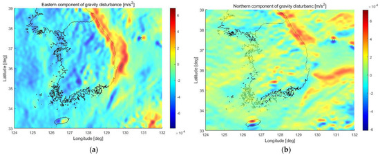
Figure 4.
Horizontal gravity disturbance map of the Korean Peninsula used for MLP neural network training: (a) represents the eastern component of horizontal gravity disturbance, and (b) depicts the northern component of horizontal gravity disturbance.
However, a significant challenge arose during its generation. The EGM2008 gravity model is mainly determined by latitude, longitude, and height, represented in spherical coordinates. When creating neural network learning data for a platform moving in 3D, generating an extensive amount of data becomes practically impossible, making neural network training unfeasible. To overcome this problem, this paper introduces a constraint by limiting the traveling path of the platform. Given the assumption that the platform, which is the focus of this study, moves exclusively on the Earth’s surface, height can be consistently specified based on the platform’s horizontal position of latitude and longitude. However, defining height is challenging in the presence of multiple references. This will be discussed further in the next section.
4.2.1. Geoid Height (Geoid Undulation)
Essentially, we have 3 main categories of elevation references: ellipsoidal height, geoid height, and orthometric height. The ellipsoidal height is the difference in the vertical distance between a point on the Earth’s surface and the ellipsoid. The ellipsoidal height is also known as the geodetic height and should not be confused with geodetic datum. When capturing coordinates with a GPS receiver, the elevation data reference the WGS84 ellipsoid, which means each captured coordinate needs to be calculated to match elevations with more accurate geoid height. The geoid height (undulation) is the difference of the vertical distance between the reference geoid and the reference ellipsoid. The geoid is a hypothetical shape of the Earth that often coincides with the average of the Earth sea level and its imagined extension above or below land areas; the geoid height may sometimes be referred to as elevation at Mean Sea Level (MSL). The orthometric height is the difference between the vertical distance from a location on the Earth’s surface and the geoid. Because the geoid coincides with MSL, whenever you see elevation data described as ‘0’ meter above or below sea level, they are referring to the orthometric height.
The relationship between ellipsoidal height (h), MSL height (H), and geoid height (N) can be defined as follows:
The geoid height can be calculated using the EGM2008 gravity model or interpolated with pre-calculated geoid height values, as described in [22]. To establish a 3D position in a spherical coordinate system, you need the latitude, longitude, and height in the navigation coordinate system. Here, the height in the navigation coordinate system refers to the ellipsoidal height. Therefore, if you have the orthographic height and geoid height of a point, you can compute the ellipsoidal height on the Earth’s surface.
Figure 5a clearly shows the definitions for each of the 3 reference heights and the relationships between each. Figure 5b illustrates the distribution of geoid undulation of geoid height around the Korean Peninsula, displaying a gradual gradient from southeast to northwest, ranging from approximately 15 m to 31 m [23].
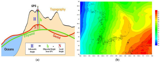
Figure 5.
The definitions of different heights: (a) illustrates the relationship between geoid height, ellipsoidal height, and orthometric height; (b) represents geoid undulation (geoid height) around the Korean Peninsula.
4.2.2. Extracting Orthometric Height from SRTM DEM
In order to calculate the ellipsoid height at a specific location, as shown in Equation (35), the orthometric height of the location must be known. Unlike geoid height, orthometric height does not have a computational model and can only be obtained through interpolation from a dataset known as a Digital Elevation Model (DEM). Therefore, in this section, we will explain DEM and how to obtain an open-source DEM for use in this paper.
At sea, the orthometric height is ‘0’. However, for land areas, the process is more complex. It involves determining the elevation of the ground surface, accounting for terrain irregularities and the shape of the ground or road. A digital elevation model (DEM) is used for this purpose. A DEM is a grid raster data representation of terrain, excluding terrain vector features (e.g., streams, ridges) and artificial structures (wires, buildings, towers), as well as natural features like trees and vegetation.
Various definitions are associated with DEMs, with two major models being the Digital Terrain Model (DTM) and Digital Surface Model (DSM). In most cases where distinguishing between bare ground and surface objects is not critical, the generic term DEM suffices. DEMs are created from remote sensing data collected via satellites, drones, airplanes, typically employing technologies like laser scanning (LiDAR), geodetic surveying, or radar interferometry (InSAR).
- Digital terrain model (DTM): DTM represents a three-dimensional portrayal of terrain or surface topography, featuring points with defined heights. DTM includes feature points such as rivers, ridges, and breaklines but excludes natural or man-made objects found on the Earth’s surface, like vegetation and buildings. It approximates the height of bare land without accounting for surface features. DTM encompasses a set of 2D points with height values approximating the vertical distance between a feature point and a datum plane or geodetic data. In certain research fields, DTMs are considered vector datasets augmented with linear features of bare ground terrain (e.g., breaklines, ridges). Photogrammetric processing of aerial and space stereo images is often used to create DTMs. It is noteworthy that DTMs can also be derived from DSMs by calculating the difference between the height values of surface objects (e.g., trees, buildings) and their surroundings.
- Digital surface model (DSM): DSM represents a three-dimensional portrayal of the Earth’s surface height, encompassing both natural and man-made objects on the Earth’s surface. It characterizes the MSL height of reflective surfaces, including vegetation, buildings, and other objects above the bare ground. DSM typically overlays a canopy model onto the bare ground surface. In this paper, we will use the Shuttle Radar Topography Mission (SRTM) DEM as an orthometric height, which employs NASA’s satellite-based InSAR DEM technique to cover around 80% of the Earth’s landmass. The SRTM DEM can be freely downloaded from the (http://earthexplorer.usgs.gov accessed on 1 July 2023) website, offering global coverage with 1 arcsec resolution [24].
- DEM vs. DTM vs. DSM: It is important to distinguish between these three models. A DEM is the all-encompassing term, including both DTM and DSM. DTM is a DEM that focuses on bare earth elevation, while DSM incorporates all surface objects. Figure 6 illustrates the difference between DTM and DSM, with DTM following the ground’s contours and DSM capturing the surface structures such as the tops of buildings and trees.
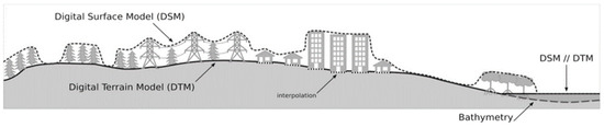 Figure 6. A schematic representation of surfaces represented by DSM (≡ SRTM) and DTM. In this paper, the orthometric height can be obtained from the SRTM DEM.
Strictly speaking, when using the SRTM DEM, there is an error equivalent to the height of surface features when converting to ellipsoid height using Equation (35) and geoid height. However, this study focused on ground vehicles or water vessels, assuming that they move on land with no obstacles or car load. Therefore, it was reasonable to assume that the DSM height provided by the SRTM DEM coincided with orthometric height within the scope of this research.
4.3. Framework of Multi-Layer Perceptron Design and Training
In this study, we designed and trained MLPs using the MATLAB Deep Learning Toolbox [25]. The target of our work was an INS that calculates navigation solutions in real time with a 5 ms period on an embedded NPU that has a PPC-P2020 dual-core 1 GHz processor [26]. To meet the strict real-time requirements, all calculations must be completed within a maximum of 1.2 ms [27]. Before designing the MLPs, we checked the computational complexity of the MLP models to predict the execution time in an embedded NPU according to the size of the neural network model.
The computational complexity, denoted as , can be calculated as follows [27]:
Based on Equation (36), preliminary research confirmed that an execution time of approximately 1.2 ms is required when the computational complexity () is 13,250 [27]. This is similar to the execution time of a neural network model with 5 hidden layers, each containing 50 nodes, when the input and output dimensions are 2 and 1, respectively. Therefore, we designed a network with parameters existing near 13,250 . As a result, four MLP networks were designed and their architectures are summarized in Table 1.

Table 1.
MLP networks: numbers of hidden layers, neurons, and time complexity.
In this network design, the input layer contains two neurons to host the input vector elements [latitude, longitude]. Layers from the 2nd to the Nth work as internal hidden layers, and each layer is fully connected. The output layer yields the eastern and northern components of the DOV. To train the neural network, the hidden layers (excluding the output layer) consist of a ‘fullyConnectedLayer’ for full connectivity, a ‘batchNormalizationLayer’ to expedite learning and resolve local optima, and a ‘swishLayer’ as an activation function. The ‘Swish’ activation function, given by Equation (37), is a Google-developed function that is shown to outperform ‘ReLU’ in deep layer training. The detailed architecture of the MLP model is presented in Figure 7.
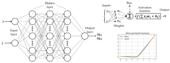
Figure 7.
MLP showing the working of the neural network using input, hidden, and output layers. The bottom left of the figure shows the weights associated with each neuron and transformation using an activation function. ‘Y’ represents the final output from the neural network and is achieved by optimizing other hyper-parameters. The bottom right of the figure shows the ‘ReLU’ and ‘Swish’ activation functions.
The MLP training tool was MATLAB R2021a. The network sizes for each case are shown in Table 1, and the learning conditions are detailed in Table 2. We utilized the ‘adam’ optimization function, suitable for regression analysis, with an initial learning rate of 0.1, decreasing by a factor of 0.4 every 5th epoch. This dynamic learning rate initially increased validation error variance but ultimately enhanced learning speed. As epochs progressed, the learning rate decreased, leading to reduced validation error deviation.
Table 2.
Training options for DOV prediction MLP networks.
To evaluate the training results, we calculated the loss using half mean squared error and validated MLP network performance with root mean squared error, as defined in Equations (38) and (39).
The MLP model training process was executed on a workstation PC based on an Intel Xeon Gold 2.5 GHz dual processor. Figure 8 illustrates the evolution of the training process, with the upper part representing RMSE prediction error and the lower part showing RMS loss. A mini-batch size of 1,238,496 was used, meaning the network received 500 database items, and neuron weight adjustments were made using the backpropagation algorithm. This resulted in 5000 training iterations, given a total of 61,924,800 datasets in the full learning dataset. To enhance learning rate stability and prevent abrupt fluctuations toward the end of training, we initialized the learning rate at 0.1 and reduced it by a factor of 0.4 every 5 epochs. Every 50 calibration iterations, we assessed network accuracy against 6,192,480 validation set items, represented in black in the plot. This evaluation determined if the network was learning effectively. The training process was configured to conclude after 5000 training iterations. Input and output data were pre-normalized to eliminate training bias.
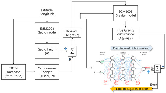
Figure 8.
The framework of obtaining data for supervised learning and the training process of an MLP.
Figure 8 illustrates an overview of creating the learning dataset and training an MLP model for supervised learning. On the left side of Figure 8, a sequence of steps outlines the creation of a learning dataset comprising input and reference values. Although in theory, the ellipsoid height is necessary to compute gravity disturbances using an SHM, in this study, it was assumed that it can be derived from surface height based on specific position. Consequently, to determine the ellipsoid height at the location, the geoid height was calculated, the orthometric height was extracted from the SRTM DEM, and these values were summed to obtain the ellipsoid height. By feeding this calculated ellipsoid height and the corresponding position (latitude and longitude) into the SHM of the EGM2008 gravity model, the true gravity disturbances were obtained for the input positions. These true gravity disturbances served as the reference output data during the supervised learning process. In the learning process, the reference value was compared with the value predicted by the MLP network, resulting in an error. Backpropagation was then executed using this error value to refine the MLP model.
Figure 9 illustrates the training results for the eastern and northern components of MLP1~MLP4, with training times of approximately 2000 min on average, except for Figure 9b. However, due to the similar MLP size in each case, we could not find a meaningful correlation between neural network size and training time in this study.
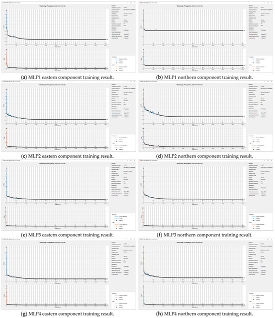
Figure 9.
Training progress graphs of the MATLAB Deep Learning Toolbox showing the supervised learning results of MLP1~MLP4 models. When training was completed, we could check the final validation accuracy: (a) 0.3087; (b) 0.8915; (c) 0.2320; (d) 0.3283; (e) 0.2796; (f) 0.3033; (g) 0.1993; and (h) 0.2899.
In Table 3, we present the final training loss values and validation accuracy for each case. From the table, it is evident that MLP4 exhibited the best training performance. In the following section, we implement MLP4 on the INS’s built-in embedded NPU and present the field test results.
Table 3.
Final validation loss and RMSE of MLP1~MLP4 training results.
Table 4 shows the specifications of the NPU built into the INS for real-time navigation and DOV calculations. To ensure real-time execution, we adopted VxWorks 6.9, a commercial real-time operating system [28]. The weights and biases of the trained MLP model were stored in binary file format in the true flash file system (TFFS) created in Nor-Flash Rom. As expected, the execution time of MLP1, with the highest computational complexity, was the longest, with execution times decreasing as the computational complexity was reduced.
Table 4.
Specifications of INS’s built-in embedded NPU used in a field test.
5. Experimental Study about Real-Time DOV Compensation Using MLP
In this chapter, the results from Section 4 are utilized to assess execution time. This involves implementing four MLP models within the NPU to verify whether they meet the execution time requirements. Furthermore, an inertial navigation system (INS) employing the MLP4 model, which demonstrated superior training performance, is installed in a test vehicle. A two-hour road driving test is conducted using the vehicle. Following the test, the performance of the MLP4 model in predicting and compensating for the DOV is verified. This is accomplished by comparing the position error of the INS with and without DOV compensation against the GPS location.
5.1. Comparison of MLP Model Execution Time Inside NPU
After completing the MLP training, we obtained the biases and weights for each layer of every MLP neural network. These weights and biases were implemented on the INS’s built-in NPU to accurately measure the execution time of each neural network. A logic analyzer was used to record the time difference before and after calculation by the MLP models, and the execution time result of MLP4 is displayed in Figure 10 as a representative example. For context, the execution times were recorded as 1.168 ms for MLP1, 1.113 ms for MLP2, and 1.064 ms for MLP3.
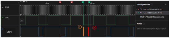
Figure 10.
Timing marker P1 indicates the time interval between points 1 and 2, measured at 1.041 ms. This implies that the horizontal gravity disturbance comprises two components: east and north. During each navigation cycle, NPU computes the MLP4 model twice, employing distinct weights and biases for each component. Consequently, the total time needed for actual gravity disturbance calculation is 2.082 ms (1.041 ms × 2).
The Figure 11 schematically illustrates the internal operational process of the NPU for navigation and gravity disturbance compensation. Inside the NPU shown in Figure 11, the navigation algorithm computation follows a series of steps:
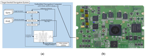
Figure 11.
Schematic of the internal operational process of the NPU inside the INS: (a) outlines the steps involved in the navigation algorithm calculation and real-time prediction of gravity disturbances within the NPU; (b) photo of actual NPU.
- (1)
- Data Reception: Output values from gyros and accelerometers are received by the NPU.
- (2)
- Navigation Algorithm Computation: Based on the received inertial sensor data, the NPU calculates attitude, velocity, and position.
- (3)
- Input Data for MLP: The calculated position values (latitude and longitude) are input into the MLP model.
- (4)
- Prediction of Gravity Disturbances: The MLP model outputs real-time predictions of gravity disturbances based on the inputted positions.
- (5)
- Compensation for Gravity Disturbances: These predictions are utilized to compensate for gravity disturbances and DOV in velocity and attitude calculations.
All of these processes occur in real time at intervals of 5 ms during the navigation task of VxWorks, that is, the RTOS of the NPU. As mentioned, the MLP4 calculation time was 2.082 ms and there was a 2.918 ms time margin, which accounted for 58% of the total execution cycle. In conclusion, the proposed MLP4 model in this paper demonstrated the capability to calculate and compensate for gravity disturbances in real time inside the NPU without the need for external auxiliary PC.
5.2. Validation of Enhanced Position Accuracy in Real-Time DOV Compensation Using MLP
To validate the real-time DOV compensation performance, a vehicle test was conducted. The test setup included a navigation-grade INS and a single-antenna GNSS receiver. The INS output position/velocity/attitude at 200 Hz, while the GNSS receiver offered reference position information at 1 Hz. The GNSS receiver provided position accuracy of 2 m horizontally and 3 m vertically, serving as a sufficient reference for evaluating INS position accuracy. The primary inertial sensor errors for the INS were a gyro drift bias of 0.003 deg/h and accelerometer drift bias of 30 µg. The trained MLP4 model was implemented on a built-in NPU of the INS for the vehicle test. The performances and characteristics of the inertial sensors and GNSS receiver are listed in Table 5.
Table 5.
Specifications of inertial sensors and GNSS receiver.
The test vehicle carried a GNSS receiver, power supply, graphic user interface (GUI) device, and the INS. The GUI was connected to both the INS and GNSS receiver to record the position, velocity, and attitude of the INS at 200 Hz, as well as the position of the GNSS receiver at 1 Hz. A laptop operated the GUI and stored various data received from it. The power supply drew 220 V voltage from the vehicle and provided DC-28V to the INS and DC-5V to GNSS receiver. The test vehicle is shown in Figure 12 and vehicle testing followed these steps:
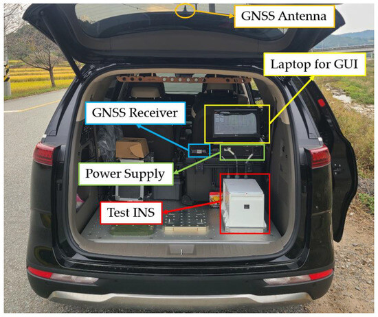
Figure 12.
Photograph capturing the inside of the test vehicle. The power supply, GNSS receiver, test INS, and laptop for the GUI were installed inside the vehicle, and the GNSS antenna was mounted on the vehicle’s roof.
- (1)
- Install the required equipment on the test vehicle.
- (2)
- Proceed to the starting point of the driving test.
- (3)
- Power up the INS and GNSS receiver, obtain current location data from the GNSS receiver, and input them into the INS through the GUI.
- (4)
- After receiving the current location, the INS undergoes initial alignment for 900 s, and the GUI initiates data logging.
- (5)
- Upon completion of alignment, commence the test and drive for 2 h.
- (6)
- When the test is completed, stop data logging in the GUI and switch off the power supply.
The test was performed on the road from Daejeon Metropolitan City to the summit of Mt. Jirisan. Figure 13 shows the field test trajectory. Most of the test took place on highways with smooth changes of attitude and speed. The vehicle’s moving trajectory began in the lowlands to the north and progressed southward, with a noticeable rapid increase in height near Mt. Jirisan.
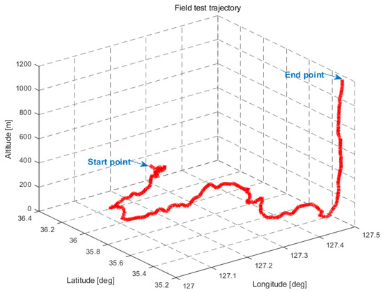
Figure 13.
Field test trajectory. The vehicle followed a route from Daejeon Metropolitan City to the summit of Mt. Jirisan.
In Figure 14, the gravity disturbance distribution within the vehicle testing area is displayed. Notably, the deviation from gravity disturbance was relatively small near the starting point, Daejeon city, but increased as the destination, Mt. Jirisan, was approached. Additionally, the deviation of the northern component of the gravity disturbance was greater than that of the eastern component. The blue circles in Figure 14a,b indicate the Mt. Jirisan area, which was the final destination area for the vehicle testing.
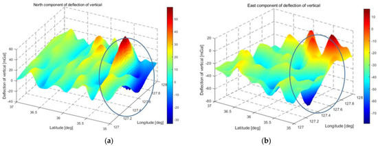
Figure 14.
The graph illustrates the distribution of horizontal gravity disturbance in the vehicle test field: (a) the east component of the horizontal gravity disturbance; (b) the north component of the horizontal gravity disturbance.
In Figure 15, a comparison is made between the real-time calculated gravity disturbance prediction by the MLP4 model during vehicle testing and the results calculated post-processing using 2160th degree and order SHM. The results in the figure can be explained for the following reasons:
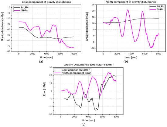
Figure 15.
Analysis of the gravitational disturbance in the horizontal plane (eastern and northern components) along the test trajectory. The data labeled as MLP4 represent real-time calculations made by the INS’s NPU, whereas SHM denotes calculations performed afterwards, specifically the 2160th order of SHM at the same location: (a) the eastern component of the horizontal gravity disturbance; (b) the northern component; (c) the prediction made by MLP4, which is then subtracted from the SHM-calculated value. The difference between these values fluctuates within a range of approximately ± 25 mGal.
- (1)
- Difference in Frequency Components: The SHM effectively captures the high-frequency components of gravity disturbance, indicating that the SHM accurately captures detailed frequency components. In contrast, the MLP4 model removes high-frequency components and reflects only slowly changing low-frequency components.
- (2)
- Training Data Coverage: The MLP4 model appears to have been trained over too wide an area, leading to a representation that is flattened overall rather than accurately reflecting the gravity disturbance distribution in specific regions. This means that the model may not capture regional uniqueness and may have learned characteristics from the broader area.
- (3)
- Weight of Terrain Data: The training data for the model include a higher proportion of terrain data, such as oceans and flatlands, where gravity disturbances change gradually. This might explain why high-frequency components have been removed from the model’s predictions.
Despite these limitations, the MLP4 model was shown to perform reasonably well when compared to the gravity disturbance error presented in [5]. This indicates that the MLP4 model exhibited acceptable performance even though it disregarded or inaccurately handled high-frequency components. These results illustrate the characteristics that can arise depending on the model’s training data, training methodology, and the specific application domain. These findings can provide insight into the strengths and limitations of the MLP model.
To assess navigation accuracy with and without DOV compensation, position error was used as the evaluation metric. Real-time DOV compensation was achieved using the MLP4 model implemented inside the NPU of the INS. To compare results with and without DOV compensation, position data were recorded on a laptop through the GUI interface.
In Figure 16, the effect of DOV compensation on INS position calculation during the vehicle test is illustrated. The black solid line is the result without DOV compensation and the solid purple line is the result of calculated navigation with real-time compensation for the DOV. In particular, the compensation for the DOV during INS navigation calculation resulted in a less position error, with a maximum radial position error showing approximately 27% improved performance compared to without DOV compensation in Table 6.
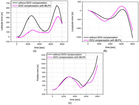
Figure 16.
Position errors during the field test are compared with GPS results. In each figure, the black line represents the result of calculating the navigation solution without compensation for the DOV. The purple line represents the result of compensating for the DOV during navigation calculation with the MLP4 network: (a) latitude error of field test results for both cases; (b) longitude error of field test results for both cases; (c) radial position error of field test results for both cases.
Table 6.
Maximum and mean latitude, longitude, and radial position errors without and with DOV compensation are compared with GPS results.
In this chapter, according to the field test results, an MLP model was implemented in the INS to compensate for the DOV and improve positional accuracy. The results of the experiments showed that compensating for the DOV led to smaller position errors compared to uncompensated results. Furthermore, the proposed MLP model demonstrated the ability to calculate the DOV in real time, and its DOV prediction performance was found to be reasonably good compared to other research results.
6. Conclusions and Future Work
In this study, we present a real-time approach for predicting gravity disturbances (i.e., DOV) utilizing an MLP neural network trained on terrain surface gravity disturbance data extracted from the EGM2008 gravity model. Our research focuses on platforms specifically operating on flat terrain, roads, or on the water, assuming predetermined heights based on latitude and longitude coordinates for vehicles or ships. This constraint allows us to represent vehicle position data as a two-dimensional trajectory, enabling the application of MLP-based learning techniques.
To ensure real-time computation, computational complexity was previously calculated to determine the MLP neural network’s size. This ensures that computation of the gravity disturbance’ eastern and northern components using MLP can be performed in about 1.2 ms. As a result, four different variations of MLP models, labeled as MLP1 to MLP4, were created. The MLP models were trained using supervised learning techniques. Each different MLP model was evaluated based on its training accuracy using metrics like HMSE and RMSE. HMSE is a variation of mean squared error, with only half of the squared errors used in the calculation. This metric is often used when the focus is on underestimating errors. RMSE is the square root of the MSE and provides a measure of the average magnitude of the errors in the model’s predictions. In this study, the MLP4 model demonstrated the smallest error, indicating that it performed the best among the four models assessed. The HMSE for the DOV’s eastern component was 0.0199 with an associated RMSE of 0.1993. For the northern component, the HMSE was 0.0420 and the RMSE was 0.2899.
Four distinct MLP models were implemented on the NPU of the INS, and their execution times were precisely measured using a logic analyzer. The measured execution times were recorded as 1.168 ms for MLP1, 1.113 ms for MLP2, 1.064 ms for MLP3, and 1.041 ms for MLP4. The results revealed a sequential reduction in execution time from MLP1 to MLP4, contrary to the size of the computational complexity. Based on these results, a vehicle test was carried out while traveling from Daejeon Metropolitan city to the summit of Mt. Jirisan. The test results revealed a reduction in position error when applying the suggested MLP4 model for DOV compensation, compared to results obtained without DOV compensation. The maximum position errors when not compensating for the DOV were as follows: latitude error was 651.6 m, longitude error was −1547.1 m, and radial position error was 1570.8 m. On the other hand, when compensating for the DOV, the maximum position errors were as follows: latitude error was 425.1 m, longitude error was −1115.2 m, and radial position error was 1146.6 m. According to these results, compensating for the DOV reduced the maximum latitude error by approximately 35.01% (i.e., (651.6–425.1)/651.6 × 100), the maximum longitude error by approximately 28.06% (i.e., (−1547.1–(−1115.2))/1547.1 × 100), and the radial position error by approximately 27.09% (i.e., (1570.8–1146.6)/1570.8 × 100). These results indicated that DOV compensation improved the accuracy of the INS.
The results of this study demonstrate that it is possible to compensate for gravity disturbances in real time by utilizing a high-precision gravity model generated by a trained MLP neural network model implemented into an INS’s built-in NUC. These research results provide valuable insights for enhancing the accuracy of the INS.
Author Contributions
Conceptualization, H.K. (Hyunseok Kim) and C.P.; methodology, H.K. (Hyunseok Kim) and C.P.; software, H.K. (Hyunseok Kim), H.K. (Hyungsoo Kim). and Y.C. (Yunhyuk Choi); validation, H.K. (Hyunseok Kim); formal analysis, H.K. (Hyunseok Kim) and C.P.; investigation, H.K. (Hyunseok Kim) and C.P.; data collection, H.K. (Hyungsoo Kim) and Y.C. (Yunhyuk Choi); data curation, H.K. (Hyungsoo Kim) and Y.C. (Yunhyuk Choi); field test, Y.C. (Yunhyuk Choi) and H.K. (Hyungsoo Kim); writing—original draft preparation, H.K. (Hyunseok Kim) and H.K. (Hyungsoo Kim); writing—review and editing, Y.C. (Yunhyuk Choi) and Y.C. (Yunchul Cho); visualization, H.K. (Hyungsoo Kim) and Y.C. (Yunhyuk Choi); supervision, Y.C. (Yunchul Cho) and C.P.; project administration, Y.C. (Yunchul Cho). All authors have read and agreed to the published version of the manuscript.
Funding
This work supported by the Agency for Defense Development Grant funded by the Korean Government (2023).
Data Availability Statement
Data sharing is not applicable to this article.
Conflicts of Interest
The authors declare no conflict of interest.
References
- Titterton, D.H.; Weston, J.L. Strapdown Inertial Navigation Technology, 2nd ed.; IEE: London, UK, 2004. [Google Scholar]
- Xu, X.; Zhang, T.; Wang, Z. In motion filter-QUEST alignment for strapdown inertial navigation systems. IEEE Trans. Instrum. Meas. 2018, 67, 1979–1993. [Google Scholar] [CrossRef]
- de Angelis, M.; Bertoldi, A.; Cacciapuoti, L.; Giorgini, A.; Lamporesi, G.; Prevedelli, M.; Saccorotti, G.; Sorrentino, F.; Tino, G.M. Precision gravimetry with atomic sensors. Meas. Sci. Technol. 2009, 20, 022001. [Google Scholar] [CrossRef]
- Kwon, J.H.; Jekeli, C. Gravity requirements for compensation of ultra-precise inertial navigation. J. Navig. 2005, 58, 479–492. [Google Scholar] [CrossRef]
- Chang, L.B.; Qin, F.J.; Wu, M.P. Gravity Disturbance Compensation for Inertial Navigation System. IEEE Trans. Instrum. Meas. 2019, 68, 3751–3765. [Google Scholar] [CrossRef]
- Jekeli, C. Precision free-inertial navigation with gravity compensation by an onboard gradiometer. J. Guid. Cont. Dyn. 2006, 29, 704–713. [Google Scholar] [CrossRef]
- Jekeli, C.; Lee, J.K.; Kwon, J.H. On the computation and approximation of ultra-high-degree spherical harmonic series. J. Geod. 2007, 81, 603–615. [Google Scholar] [CrossRef]
- Hanson, P.O. Correction for deflection of the vertical at the runup site. In Proceedings of the 1988 Record Navigation into the 21st Century Position Location and Navigation Symposium (IEEE PLANS ’88), Orlando, FL, USA, 29 November–2 December 1988. [Google Scholar]
- George, G. High accuracy performance capabilities of the military standard ring laser gyro inertial navigation unit. In Proceedings of the Position Location and Navigation Symposium, Las Vegas, NV, USA, 11–15 April 1994. [Google Scholar]
- Zhou, X.; Yang, G.; Wang, J.; Li, J. An improved gravity compensation method for high-precision free-INS based on MEC–BP–adaboost. Meas. Sci. Technol. 2016, 70, 125007. [Google Scholar] [CrossRef]
- Zhou, X.; Yang, G.; Cai, Q.; Wang, J. A novel gravity compensation method for high precision free-INS based on extreme learning machine. Sensors 2016, 16, 2019. [Google Scholar] [CrossRef] [PubMed]
- Förste, C.; Abrykosov, O.; Lemoine, J.-M.; Flechter, F.; Balmino, G.; Barthemes, F. EIGEN-6C4 The latest combined global gravity field model including GOCE data up to degree and order 2190 of GFZ Potsdam and GRGS Toulouse. In Proceedings of the 5th GOCE User Workshop, Paris, France, 25–28 November 2014. [Google Scholar]
- Wang, J.; Yang, G.; Li, X.; Zhou, X. Application of the spherical harmonic gravity model in high precision inertial navigation systems. Meas. Sci. Technol. 2016, 27, 095103. [Google Scholar] [CrossRef]
- Wang, J.; Yang, G.; Li, J.; Zhou, X. An Online Gravity Modeling Method Applied for High Precision Free-INS. Sensors 2016, 16, 1541. [Google Scholar] [CrossRef] [PubMed]
- Wu, R.; Wu, Q.; Han, F.; Liu, T.; Hu, P.; Li, H. Gravity compensation using egm2008 for high-precision long-term inertial navigation systems. Sensors 2016, 16, 2177. [Google Scholar] [CrossRef]
- Tie, J.; Wu, M.; Cao, J.; Lian, J.; Cai, S. The impact of initial alignment on compensation for deflection of vertical in inertial navigation. In Proceedings of the IEEE 8th International Conference on Cybernetics and Intelligent Systems, Robotics Automation and Mechatronics, Ningbo, China, 19–21 November 2017. [Google Scholar]
- Hofmann-Wellenhof, B.; Moritz, H. Physical Geodesy, 2nd ed.; Springer: Vienna, Austria; New York, NY, USA, 2006. [Google Scholar]
- Casado, R.; Bermúdez, A. Neural Network-Based Aircraft Conflict Prediction in Final Approach Maneuvers. Sensors 2020, 9, 1708. [Google Scholar] [CrossRef]
- McCulloch, W.S.; Pitts, W. A logical calculus of the ideas immanent in nervous activity. Bull. Math. Biol. 1943, 5, 115–133. [Google Scholar] [CrossRef]
- Werbos, P.J. Beyond Regression: New Tools for Prediction and Analysis in the Behavioral Sciences. Ph.D. Thesis, Harvard University, Cambridge, MA, USA, 1974. [Google Scholar]
- Lee, K.T.; Kim, M.S.; Kim, H.J.; Kim, J.H. A Model to Predict Occupational Safety and Health Management Expenses in Construction Applying Multi-Variate Regression Analysis and Deep Neural Network. J. Archit. Inst. Korea 2021, 37, 217–226. [Google Scholar]
- Kim, H.S.; Park, C.S. A Study on Real-time Calculation of Geoid applicable to Embedded Systems. J. Adv. Navig. Technol. 2020, 24, 374–381. [Google Scholar]
- National Geographic Information Institute. Available online: https://map.ngii.go.kr/ms/mesrInfo/geoidIntro.do (accessed on 11 October 2023).
- USGS. Available online: https://earthexplorer.usgs.gov (accessed on 1 July 2023).
- The MathWorks Inc. Deep Learning Toolbox. Available online: https://www.mathworks.com/products/deep-learning.html (accessed on 1 September 2023).
- NXP Semiconductors. QorIQ P2020. Available online: https://www.nxp.com/products/processors-and-microcontrollers/power-architecture/qoriq-communication-processors/p-series/qoriq-p2020-and-p2010-dual-and-single-core-communications-processors:P2020 (accessed on 1 September 2023).
- Kim, H.; Park, C. DNN Based Geoid Undulation Prediction Accuracy Evaluation Using EGM08 Gravity Model. Trans. Korean Inst. Electr. Eng. 2022, 71, 1157–1163. [Google Scholar] [CrossRef]
- The Wind River Systems, Inc. VxWorks. Available online: https://www.windriver.com/products/vxworks (accessed on 1 September 2023).
Disclaimer/Publisher’s Note: The statements, opinions and data contained in all publications are solely those of the individual author(s) and contributor(s) and not of MDPI and/or the editor(s). MDPI and/or the editor(s) disclaim responsibility for any injury to people or property resulting from any ideas, methods, instructions or products referred to in the content. |
© 2023 by the authors. Licensee MDPI, Basel, Switzerland. This article is an open access article distributed under the terms and conditions of the Creative Commons Attribution (CC BY) license (https://creativecommons.org/licenses/by/4.0/).