Article

Linear Active Disturbance Rejection Control for a Laser Powder Bed Fusion Additive Manufacturing Process

by
S. Zahid Hussain
1,
Zareena Kausar
1,*,
Zafar Ullah Koreshi
1,
Muhammad Faizan Shah
2,
Ahmd Abdullah
1 and
Muhammad Umer Farooq
2,*
1
Department of Mechatronics and Biomedical Engineering, Air University, Islamabad 44000, Pakistan
2
Institute of Mechanical and Manufacturing Engineering, Khwaja Fareed University of Engineering and Information Technology, Rahim Yar Khan 64200, Pakistan
*
Authors to whom correspondence should be addressed.
Electronics 2023, 12(2), 471; https://doi.org/10.3390/electronics12020471
Submission received: 5 December 2022 / Revised: 11 January 2023 / Accepted: 12 January 2023 / Published: 16 January 2023
(This article belongs to the Special Issue Feature Papers in Systems & Control Engineering)

Abstract

:
Functional metal parts with complicated geometry and internal features for the aerospace and automotive industries can be created using the laser powder bed fusion additive manufacturing (AM) technique. However, the lack of uniform quality of the produced parts in terms of strength limits its enormous potential for general adoption in industries. Most of the defects in selective laser melting (SLM) parts are associated with a nonuniform melt pool size. The melt pool area may fluctuate in spite of constant SLM processing parameters, like laser power, laser speed, hatching distance, and layer thickness. This is due to heat accumulation in the current track from previously scanned tracks in the current layer. The feedback control strategy is a promising tool for maintaining the melt pool dimensions. In this study, a dynamic model of the melt pool cross-sectional area is considered. The model is based on the energy balance of lumped melt pool parameters. Energy coming from previously scanned tracks is considered a source of disturbance for the current melt pool cross-section area in the control algorithm. To track the reference melt pool area and manage the disturbances and uncertainties, a linear active disturbance rejection control (LADRC) strategy is considered. The LADRC control technique is more successful in terms of rapid reference tracking and disturbance rejection when compared to the conventional PID controller. The simulation study shows that an LADRC control strategy presents a 65% faster time response than the PID, a 97% reduction in the steady state error, and a 98% reduction in overshoot. The integral time absolute error (ITAE) performance index shows 95% improvement for reference tracking of the melt pool area in SLM. In terms of reference tracking and robustness, LADRC outperforms the PID controller and ensures that the melt pool size remains constant.

1. Introduction

The term “additive manufacturing” refers to a group of low-cost, very adaptable technologies that can be used to quickly prototype and create complex three-dimensional (3D) items [1]. Materials are typically applied layer by layer until a final 3D part is produced. Laser powder bed fusion (LPBF) is one of the AM processes that can produce parts in polymers and metallic materials. A subtype of LPBF additive manufacturing technology is selective laser melting (SLM). It produces functional, final metallic parts rather than parts for rapid prototyping. In SLM, powder is spread on a bed and a laser scans the predefined pattern for that layer. After the laser scan of each layer is completed, the SLM build platform containing the powder is repeatedly lowered until the final part is completed. AM processes have the advantage of producing complex parts with minimal material waste as compared to conventional manufacturing methods. SLM technology is gaining more attention in the aerospace and biomedical industries, as it permits the production of parts with complicated characteristics that would otherwise be impossible to produce using traditional manufacturing [2,3,4].
The SLM process is very complex due to the underlying physics and has over 130 parameters to optimize to produce a fully dense part [5]. It is difficult for SLM systems to produce reliable and fully dense parts because optimizing such a large number of parameters is challenging and time consuming [6,7]. Postprocessing operations, like laser shock peening (LSP), laser polishing, hot isostatic pressing (HIP) [8], and post-machining operations [9] are often implemented for the enhancement of dimensional accuracy and the surface quality of parts. The reliability of SLM-produced parts is further compromised due to the existence of defects such as distortion, porosity, cracks, and balling the effect [10,11]. The main reason for the imperfections is a nonuniform melt pool size, frequently observed due to the heat accumulation in thin or overhanging features of a part. This residual heat comes from adjacent tracks in a layer and from previously scanned layers [12,13]. This residual heat combines with the constant laser power and the size of the melt pool increases. The cooling and solidification rates decrease [14,15,16] and the microstructure of the part is altered, which leads to uncertainty in the mechanical properties of SLM-built parts.
The majority of SLM systems utilize process maps produced by heuristics and experimentation, and they operate in an open loop. As a result, the mechanical characteristics and geometrical accuracy of identical parts manufactured by the same SLM equipment differ. This unwanted behavior is due to nonuniform melt pool dimensions, which originate from process uncertainties and heat accumulation. To maintain melt pool shape consistency despite disturbances and uncertainties and to prevent the formation of defects like porosity, it is crucial to incorporate process monitoring and feedback control of laser scanning parameters into the SLM process [17,18,19]. Implementation of feedback control strategies is challenging due to the lack of control-oriented models in the SLM process. The SLM process physics can be modelled by finite element method-based models with high fidelity, but they are computationally expensive [20,21,22]. Feedback control in the SLM process also becomes challenging due to a lack of in situ measurement of the SLM process [23,24,25].
The melt pool area regulation by the feedback controllers for the SLM process is reported in the literature. Kruth et al. [26] used optical sensors to monitor the melt pool, and based on the experimental data and its system identification, they developed a model for feedback control. By detecting the melt pool characteristics and adjusting the laser power based on the sensor signal, Craeghs et al. [27] developed a feedback control system with a high-speed CMOS camera and photodiode on overhang structures in SLM. In some studies, a feed-forward control strategy was implemented [28,29,30,31]. Wang et al. [28] used a lumped parameter-based model of the melt pool along with residual heat from neighbouring tracks to adjust the laser power and obtained the laser power trajectories for a multi-track scan. This laser trajectory is then used in feedforward control on the SLM system. Iterative learning-based control schemes [32,33,34,35] used experimental or simulation data to obtain a model by using system identification techniques, and subsequently, control was implemented. Yeung et al. [36] used a high-speed coaxial camera and implemented jerk limited control to achieve better position and velocity precision. This study also considered heat from solidified metal and altered the laser power. Renken et al. [37,38,39] used in process measurement of the pyrometer and implemented feedback and model-based feedforward control of LPBF processes. Zhimin Xi implemented PID and MPC control strategies for the LPBF process using a machine learning model built from melt pool experimental data [40]. Despite process uncertainties, the control goal was to maintain the melt pool’s breadth and depth.
All the control effort for SLM was focused on maintaining the melt pool dimensions. The models used for SLM process control have many assumptions, which are based on either simplified physics or experimental or simulated data. Therefore, in all the models, elements of unmodeled dynamics and parameter uncertainty are present. Further residual heat from already scanned tracks and layers acts as a disturbance in the melt pool dynamics. Some other unmeasurable external disturbances are deviations in environmental conditions due to fumes and inherent gases in the build chamber. Thus, model uncertainties and internal and external disturbances call for disturbance rejection control schemes to produce defect-free, reliable, and high-quality parts from SLM systems.
A control method known as active disturbance rejection control (ADRC) seeks to eliminate generalized disturbances, such as model uncertainty and internal and external disturbances [41]. In the ADRC design, internal uncertainties and external disturbances are interpreted as total disturbances, which are estimated by an extended state observer (ESO) and cancelled in real time. The ADRC approach has drawn a lot of interest, as it improves the drawbacks associated with the PID error feedback structure. In the PID control, the plant is subjected to the control action after the disturbance has affected it. The ADRC incorporates a nonlinear feedback mechanism and combines the state observer and error driven control law concepts from the current control theory and PID. Initially, the ADRC was developed by Han [42,43,44]; it has nonlinear functions and their tuning is complex. Gao in [44,45] formulated a linear framework of the ADRC as linear active disturbance rejection control (LADRC), which is superior to the NLADRC in parameter tuning and theoretical analysis [44]. LADRC is a useful design technique that has been successfully used in a variety of engineering domains, particularly high-speed and high precision control, such as aerospace [46], electric motors [47,48,49], power plants [50], robotics [51,52,53,54,55], and quad rotors [56]. The LADRC has been demonstrated as a strong alternative to PID in terms of performance and viability, offering a new approach to solving engineering problems with high precision and powerful disturbance rejection capabilities [41,42,57,58,59].
ADRC comprises three parts, which include the tracking differentiator (TD), the extended state observer (ESO), and the ESO-based feedback control. The critical component of ADRC that estimates both the system states, and an extended state is the extended state observer (ESO). The extended state represents the combined effect of the unmodeled dynamics, parameter uncertainties, and external disturbances as a generalized disturbance. These lumped disturbances are estimated by the ESO and cancelled in the inner loop. Other estimated system states are used in feedback control.
In order to control the melt pool dimensions in the presence of process uncertainty and disturbances in the form of residual heat from previously scanned tracks, a linear active disturbance rejection control (LADRC)-based control method was used. LADRC was chosen because of its good uncertainty handling, disturbance rejection, and robustness capabilities. Further, the LADRC algorithm is simple, fast, and suitable for rapidly changing dynamic systems like those in SLM. The tuning of LADRC is simpler than that of ADRC, as it has fewer parameters to tune. The model of the melt pool cross-section area used in this work is based on a lamped parameter modelling approach [28] and is obtained by applying energy balance to a half ellipsoidal volume. The ADRC algorithm was used to achieve real-time control of the melt pool width during wire arc additive manufacturing [60] based on a model retrieved from deep learning. Other examples of disturbance rejection include repetitive control [61,62] and iterative learning control [34]. They are based on a data-driven model and controlling the laser galvo. To the best of the authors’ knowledge, this is the first implementation of ADRC in the SLM additive manufacturing process. The simulation findings show that the LADRC is effective in regulating the melt pool area in the presence of a disturbance. The following are this paper’s main contributions:
  • The model of the melt pool in the SLM system is calibrated by experimental benchmark data.
  • The LADRC framework is used to regulate the melt pool cross section area in the SLM system.
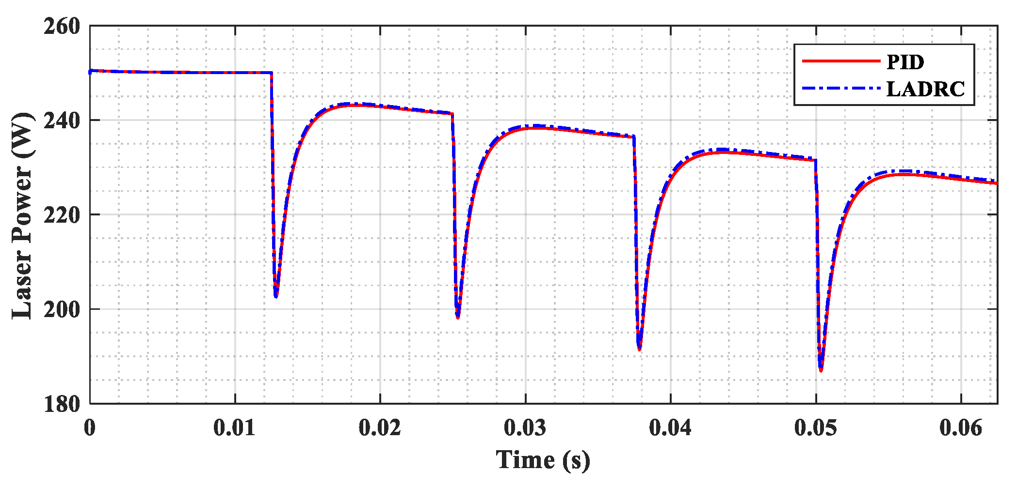
  • The LADRC performance is evaluated and compared with conventional PID controller.
The rest of the paper is arranged as follows: in Section 2, the mathematical model of the SLM melt pool and, the LADRC control strategy are presented. In Section 3, the control paradigm and simulation results are presented and the effectiveness of the control strategy is discussed. In Section 4, this work is concluded.

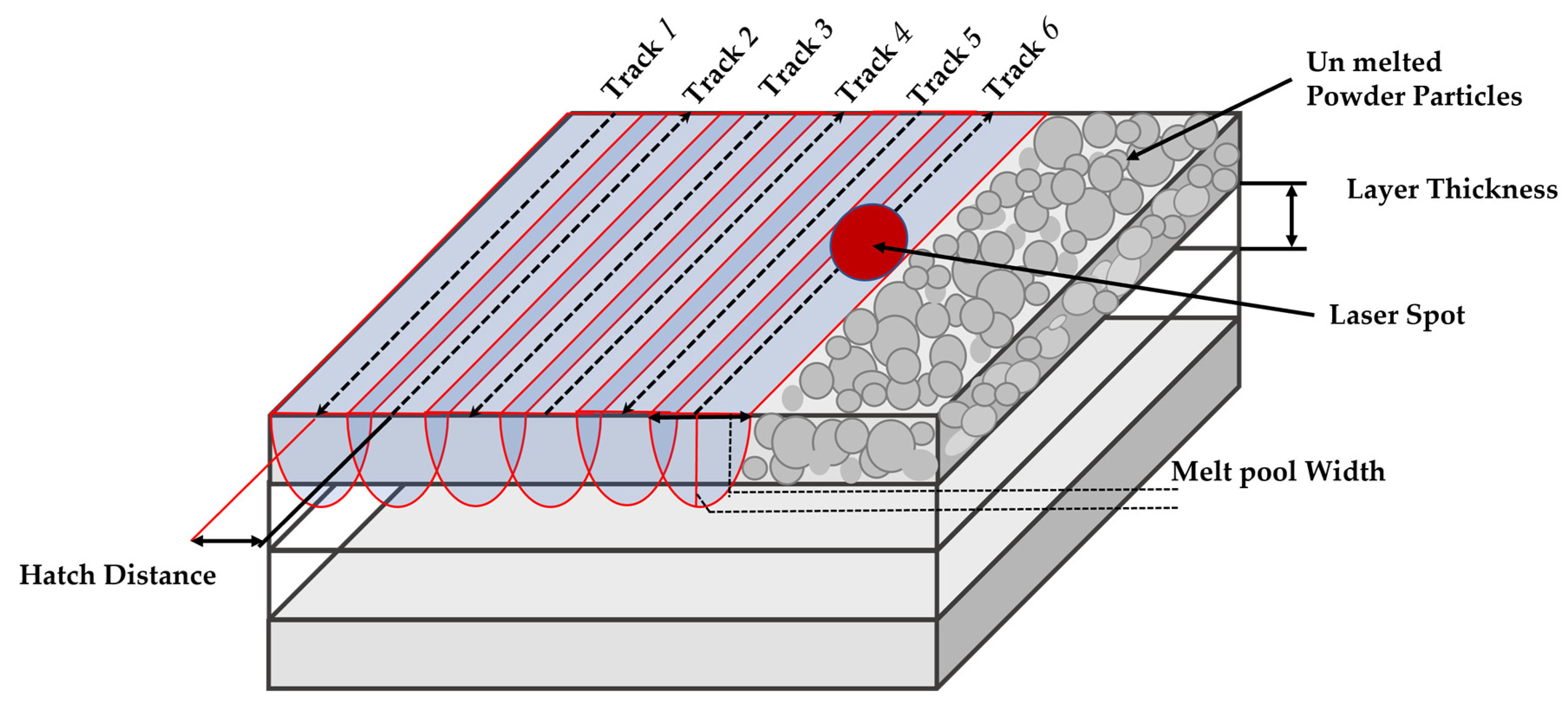
2. Materials and Methods

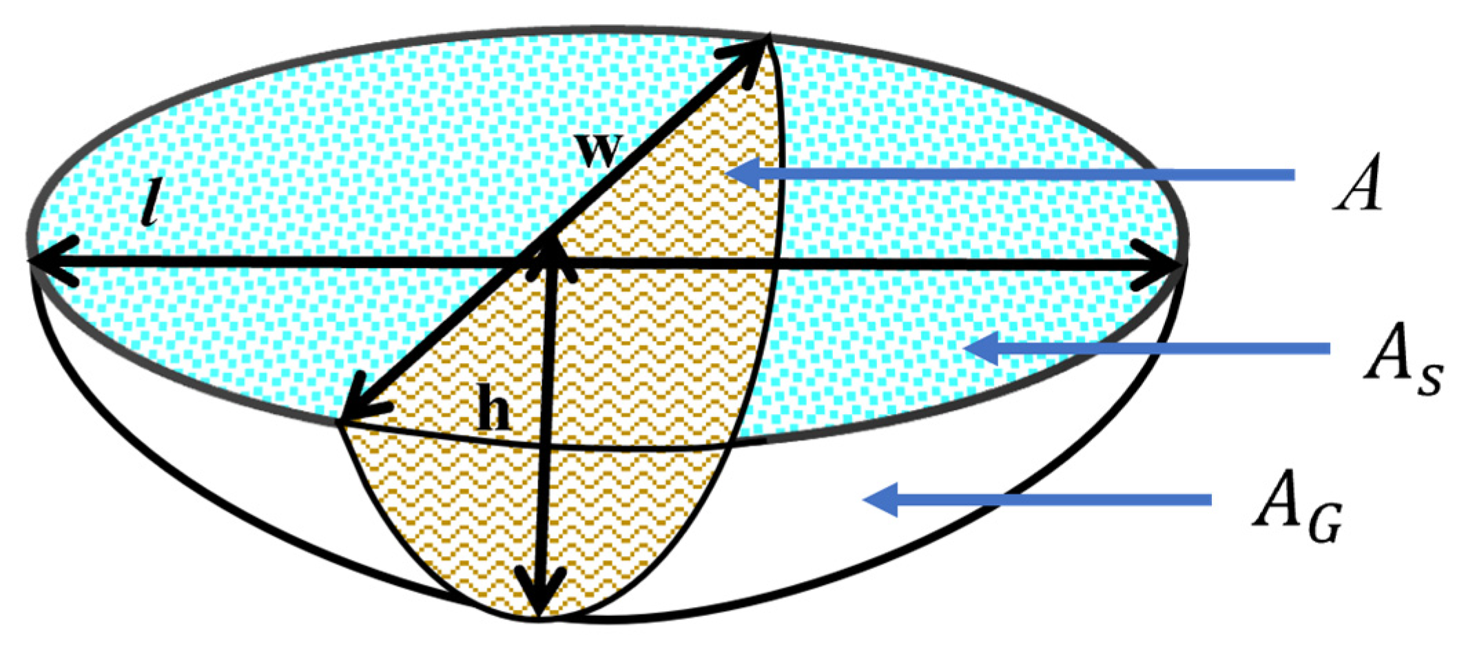
2.1. SLM Melt Pool Model Description and Assumptions
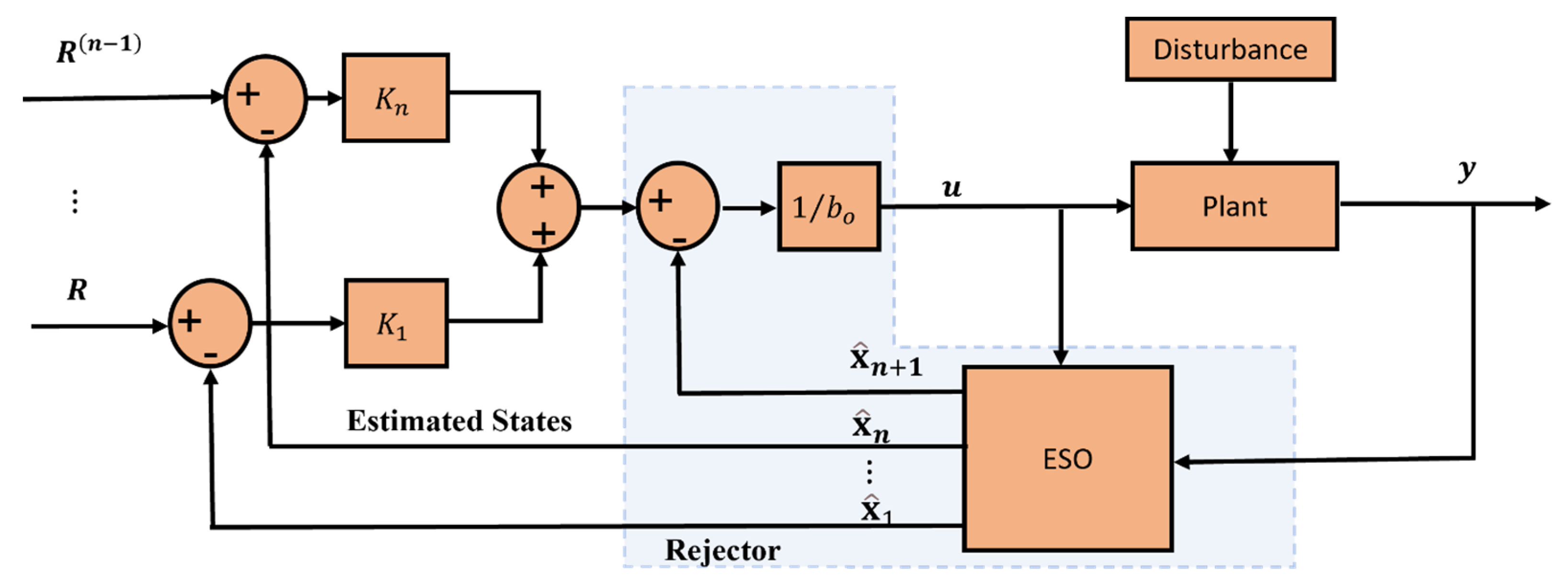
This section describes the derivation of a control oriented model of melt pool dynamics as proposed by Wang and Doumanidis [63,64]. The model was established based on lumped parameters and the melt pool’s energy balance in the SLM process. After that, the model was linearized under steady-state melt pool conditions. In order to improve model fidelity, a disturbance model was introduced to the process dynamics to account for the overlooked thermal interactions.
The SLM process parameters are shown in Figure 1. The model input and output were laser power and melt pool cross-section area, respectively. The model was implemented by assuming energy balance on a melt pool with a half-ellipsoidal shape, a uniform width-to-length ratio, and a constant width to depth ratio, both of which are defined as β = l w and r = w d , respectively. The energy balance of the melt pool volume is expressed as in Equation (1):
d d t ρ V t e t = ρ A t ν   t e b + P s
where e t is the specific internal energy of the melt pool, e b is the specific energy of the solidified material, and P s is the total thermal power exchange at the melt pool boundaries given in Equations (2)–(4).
e t = c s   T m T a + h S L + c l T t     T m
P s = η Q t A s α s   T t T i n i t A G α G   T t T a A G ε σ T 4 t T a 4
e b = c s   T m T i n i t
The definitions of the variables and parameters in Equations (2) and (3) are given in Table 1.
T i n i t is equal to T a for the first track; however, energy from previously scanned tracks causes this temperature to increase from the second track onward.
The model is simplified using a geometric definition of a half ellipsoid volume and cross-section area using l , w , and d as the length, width, and depth of the half ellipsoid, respectively. The model assumes a constant length-to-depth ratio of β = l w and a constant width-to-depth melt pool defined as r = w d .
3 2 λ ρ e A 1 2 t   d A t d t = ρ A t ν   t e b + η Q t A s α s   T t T i n i t A G α G   T t T a A G ε σ T 4 t T a 4
It is assumed that temperature T t approached steady-state temperature T s s   , which can be represented using a constant percentage of melting temperature T m , as in Equation (6). The reason for this assumption is that temperature T t   evolves and reaches a steady state much faster than the melt pool volume.
T s s   T m   = μ T m
The melt pool cross-section area   A , top surface area A s t and curved surface area   A G t are shown in Figure 2. The melt pool areas A s t ,   A G t and volume V t in terms of β and r are expressed as λsA(t), λGA(t) and λA 3 2 (t), respectively. Here, λ ,   λ S   and   λ G are defined as 4 3 r / π 1 2 β , 2 5 3 r 1 3 β 2 3 and r β , respectively.
After substitutions of assumptions and geometric definition, Equation (5) can be expressed as:
d A t d t = f A t , T i n i + g A t . Q t
where f A t , T i n i and g A t are further elaborated in Equations (8) and (9).
f A t , T i n i t = 3 2 λ ρ e 1 { ρ ν   c s T m T i n i t + λ s α s 1 + μ T m T i n i t + λ G α G 1 + μ T m T a + λ G ε σ 1 + μ 4 T m 4 T a 4 } A 1 2
g A t = 3 2 λ ρ e 1 . η A 1 2
In the above model, the heat from the first track changes the initial temperature T i n i t of the second track. The T i n i t of track n is affected by heat from the previously scanned (n − 1) tracks, as shown in Figure 3. T i n i t in each track is modelled by a transient moving point heat source solution developed by Carslaw and Jaeger [53]. The melt pool area is disturbed from steady-state conditions by this increased T i n i t in each track if the same laser power is used.
The simulations were conducted on Inconel 625 metal, and the thermal properties of Inconel 625 are adopted from [28,65]. The Inconel 625 and other simulation data are listed in Table 2. The thermal conductivity k and specific heat Cp values are temperature dependent. Their values vary from 25 °C to melting temperature, so we have considered the average values of these parameters in the simulation.
The parameters “r” (melt pool width-to-depth ratio) and “β” (melt pool length-to-width ratio) are calibrated by experimental benchmark data sets [66,67]. There are several studies that show that, for defect-free part production in SLM, the melt pool should be in conduction mode [68]. In conduction mode, the width-to-depth ratio of the melt pool is approximately equal to 2. The chemical composition of Inconel 625 is shown in Table 3.

2.2. ADRC Control

The ADRC structure has three components: first, the tracking reference signal; second, the extended state observer (ESO), which gives estimates of both the state and total disturbance in terms of output; and third, a full-state feedback controller based on the ESO. If a linear function is used in ESO, the ADRC is referred to as “linear active disturbance rejection control” (LADRC). The LADRC has inherent robustness properties and is the preferred control strategy in the presence of disturbances and uncertainty in the system dynamics. In this part, the conceptual foundations, the design of the ESO, and the control law synthesis of the ADRC are presented.

2.2.1. Linear ADRC-Preliminaries

Consider the nth order dynamic system to develop the LADRC control strategy.
y n t = f y t , u t , w t + b o u t
where y is the measured output and u is the input. f t as an unknown time-varying function that represents generalized disturbance. It depends on states, internal uncertainties, unmodeled dynamics, control input, external disturbances (w), and system dynamics. b o u t is the control input and b o is a design parameter. The core concept of ADRC is that disturbances can be estimated and canceled. The states of a general system are shown in Equation (10). Unmodeled dynamics and external disturbance are added as augmented state x n + 1 in the system dynamics. Let x 1 = y ,     x 2 = y ˙ ,   ,   x n = y n + 1 , x n + 1 = f in Equation (10) be represented as [44,69]:
x ˙ 1 = x 2 x ˙ 2 = x 3 x ˙ n = x n + 1 + b u x ˙ n + 1 = f ˙ y = x 1
A state space realization of dynamics system in Equation (11) can also be expressed as:
x ˙ = A x + B u + E h y = C x
The extended order system in Equation (12) comprises of extended state vector x 1   x 2     x 3   x n + 1 and system matrixes A, B, E, and C in the extended system are defined as follows:
A = 0 0 0 0 1 0 0 0 0 1 0 0 0 0 1 0 n + 1 n + 1 ,       B = 0 0 b 0 n + 1 × 1 ,           E = 0 0 0 1 n + 1 × 1 ,           a n d C = 1 0 0 0 1 × n + 1
The main assumptions of LADRC are as follows:
  • It is assumed that f is differentiable with h = f ˙ , the derivative of an unknown disturbance.
  • The extended system presented in Equation (12) is observable.
  • The linear extended state observer (ESO) converges.

2.2.2. Extended State Observer Design

The ESO can estimate the disturbance in real-time based on the input and output of the system without any information about the disturbance if the state-space model of the system, as in Equation (12), is accessible. The linear ESO is based on the Luenberger observer, which has a simple design and fewer tunable parameters. The ESO comprises predictor and corrector terms, as in Equation (13) [70].
x ^ ˙ = A X ^ + B u + L y y ^ y ^ = C x ^ + D u
If D = 0
x ^ ˙ = A L C X ^ + B u + L y
The matrices in this extended system are as follows:
A = 0 I n × n 0 0 ,     B = 0 n 1 × n     b       0 T   C = 1       0 1 × n ,       D = 0 ,   L = l 1     l 2           l n + 1 T
where L = l 1   l 2     l n + 1 T is the observer gain vector and x ^ = x ^ 1   x ^ 2     x ^ n + 1 T is an estimated or observer state vector. The observer gain vector is tuned to make the observer states in Equation (13) track the system state in Equation (12).

2.2.3. ADRC Control Law

The general nth order LADRC is shown in Figure 4. There is a rejector component that estimates and rejects disturbances, as well as a feedback control component that is based on the estimated states.
ADRC control law is formulated based on the estimated states and disturbances [45].
u t = u o t x ^ n + 1 b o
where
    u o t = K 1 R x ^ 1 + K 2 R ˙ x ^ 1 + + K n R n 1 x ^ n
Here K 1 ,     K 2 , ,   K n are the controller gains. Substituting u t in Equation (10)
y ˙ = f t + b o . u o t x ^ n + 1 b o
If the ESO is tuned properly, then x ^ n + 1 = f ^ t   f t and f t f ^ t is negligible.
y ˙ = f t f ^ t + u o t u o t y ˙ = K 1 R x ^ 1 + K 2 R ˙ x ^ 1 + + K n R n 1 x ^ n
In Equation (13), the ESO has n + 1 tuning gains, and in Equation (17), the control law has n tuning gains. Thus, the total number of tuning gains in the LADRC are 2 n + 1 and the number of tuning gains increases proportionally as the order of the controlled system increases. The tuning of ADRC gains is simplified by the bandwidth tuning method proposed in [39]. This tuning method parameterized the observer and controller gains.

2.2.4. Controller Design for SLM Melt Pool Dynamics

In this section, the LADRC simulation strategy is described for the SLM melt pool dynamics described in Equation (7). The model is linearized at a steady-state melt pool area of 1.1 × 10 8   m2. The linearized transfer function of the SLM dynamics is the first order, as given in Equation (19).
A s P s = 3.935 × 10 8 1 + 13.11 s
Here, n = 1 and the nth order system and the LADRC described in Equation (11) can be simplified as:
y ˙ = f t , y , w + b o u
Here, f t , y , w is a generalized disturbance representing unknown dynamics and external disturbance w , b o = 3.935 × 10 8 13.11 . The augmented system dynamics in state space is as follows [71]:
x ˙ 1 t x ˙ 2 t = 0 1 0 0 x 1 t x 2 t + b o 0 . u t + 0 0 . f ˙ t y t = 1 0 x ˙ 1 t x ˙ 2 t
Here, x 1 is the melt pool area and x 2 is the extended state representing internal uncertainty and unmodeled dynamic and external disturbances.
The expressions of the ESO for melt pool dynamics in LADRC is based on the Luenberger observer. In Equation (22), l 1 and l 2 are observer gains.
x ^ ˙ 1 t x ^ ˙ 2 t = 0 1 0 0 x ^ 1 t x ^ 2 t + b o 0 . u t + l 1 l 2 . y t y ^ t = l 1 1 l 2 0 x ^ 1 t x ^ 2 t + b o 0 . u t + l 1 l 2 . y t
Here, A = 0 1 0 0 ,   B = b o 0 ,   C = 1 0 , L = l 1 l 2 , A L C = l 1 1 l 2 0
The structure of the first order LADRC is shown in Figure 5. After estimation of the states, the control law is expressed as:
u t = u o t f ^ t b o ,   with               u o t = K P r t y ^ t
by substituting Equation (23) in Equation (20).
y ˙ = f t + b o . u o t f ^ t b o   Here   x ^ 2 = f ^ t   f t
y ˙ = f t f ^ t + u o t u o t = K P r t y ^ t
If f ^ t   f t , then the first order close-loop dynamics can be obtained by placing a close-loop pool at − K P . The two gains, the controller bandwidth ω C L , and the observer bandwidth ω E S O are tuned using the bandwidth, as suggested in [39]. The term “bandwidth parameterization” refers to the placement of all observer poles at a single position. Observer poles ω E S O should be placed to the left of the close loop poles   ω C L , as the observer dynamics must be fast and have minimum sensitivity to noise. For the first order system, it is recommended that [54]:
ω E S O 3 10 ω C L   w i t h   ω C L = K p 4 T s e t t l e
The observer poles for common pole location can be determined by the error dynamics matrix A L C . The characteristic polynomial is:
d e t s I A L C = s 2 + l 1 · s + l 2 = s ω E S O 2 = s 2 2 ω E S O · s + ω E S O 2
From Equation (27):
l 1 = 2 ω E S O   l 2 = ω 2 E S O

2.2.5. Stability Analysis

Consider the observer error e = x x ^ . The error dynamics can be expressed as
e ˙ = A L C e
The observer requires that the parameters of the gains vector L are chosen in such a way that A L C forms a Hurwitz matrix [54], that is to say, the poles ω E S O of its polynomial characteristic of A L C are all with strictly negative real parts [39]. The stability of the LADRC control strategy and the ESO convergence are presented following [71,72,73]. The existence of adequate gains ensuring estimate error convergence is justified by the Lyapunov stability technique. According to the Lyapunov theory, for asymptotic convergence of the estimated error, “e” should approach zero as the time approaches infinity.
Lemma 1. 
The observer gain in Equation (22) is selected such that A e = A L C is Hurwitz for bounded h. The ESO is also bounded.
To prove the Lyapunov stability, consider Lyapunov function V as:
V = e T X e
The solution X of the Lyapunov equation is given by:
A e T X + X A e = P
Here, P is positive definite matrix. To demonstrate the stability, the Lyapunov function in Equation (30) is differentiated and it is proved V ˙ < 0 .
V ˙ = e T P e + 2 d T P e V ˙ = e T P 1 2 d T X P 1 2 e T P 1 2 d T X P 1 2 T + d T X P 1 2 d T X P 1 2 T
which implies that V ˙ < 0 if:
e T P 1 2 d T X P 1 2 2 > d T X P 1 2 2
or
e T P 1 2 2 > 2 d T X P 1 2 2
The derivative of the Lyapunov function V ˙ in Equation (32) will be negative if
e 2 < 2 X d 2
This is true if P is the identity matrix. Thus, error e in Equation (35) is bounded as e 2 decreases. Lemma 1 can be generalized for any system described by:
β ˙ > N β + f β
with β R n and N R n × n . The subsequent lemma is:
Lemma 2. 
If matrix N is Hurwitz and function f β is bounded, then the state β in Equation (36) is also bounded.
The boundedness of the LADRC can be defined by [57] combining Lemmas 1 and 2:
Theorem 1. 
A stable closed loop system with bounded input and output is presented by the linear ADRC design in Equation (21) if the control law Equation (23) and observer Equation (22) are both stable.

3. Results & Discussion

The simulation results of LADRC controller-based close-loop SLM melt pool dynamics are presented and discussed in this section. The simulation was performed to prove the effectiveness of the LADRC controller in realizing melt pool area tracking in the presence of disturbances using MATLAB/Simulink®. In this study, the first five tracks on a metal substrate, each 10 mm in length, were simulated. The rejection of the disturbing effect of the intra layer heat coming from neighbouring tracks was observed in simulation using LADRC. A reduction in the laser input power was expected. A nominal laser power of 250 watts was selected, and the laser moved at a constant speed of 800 mm/s. The settling time t s of the melt pool dynamics is a very important parameter for feedback control. The typical melt pool length is 200 µm. For effective control action, the controller must react within a quarter (50 µm) of the melt pool length [34]. If the laser scanning speed is 800 mm/s, then the corresponding settling time is 0.625 µs. This settling time is used to calculate the values of ω C L and ω E S O   given in Equation (27).
The simulation results given in Figure 6 show that the overshoot, steady state error, and settling time were too small to be visible in a range of 0.5 × 10⁻⁸ m2 to 1.2 × 10⁻⁸ m2. However, the highlighted region in Figure 6 shows that the LADRC damped the disturbance due to residual heat from the first track and the corresponding parentage overshoot was 0.0048, the steady-state error was 6.95 × 10 14 m2, and the settling time was 2.59 × 10 4 s. This shows that the controller has exceptional robustness performance, and the developed control system has high dynamic and steady-state tracking capabilities.
Moreover, the melt pool area tracking results obtained with the LADRC controller and PID controllers with the same initial conditions are compared in Figure 7. The comparative analysis shows that both the PID and LADRC controllers tracked their references, but the control by the ADRC presented a faster time response than the PID and was more precise, with a more than 90% decrease in steady-state error and without fluctuations. The highlighted region in Figure 7 verifies improvements, as it reflects the small overshoot and settling time in the case of the LADRC as compared to the PID control. The performance of both controllers in terms of steady-state error, percentage overshoot, integral time absolute error (ITAE), rise time, and settling time is given in Table 4. The results show that the transient performance of the LADRC is better than that of the PID control. In conclusion, the LADRC is more robust and stable in the presence of the disturbance.
The closed loop system tracking error in the melt pool area for tracks 1–5 of a layer is given in Figure 8. It shows the melt pool area tracking error for both the PID and LADRC controllers. The tracking error was small in the case of ADRC as compared to a PID-based system’s melt pool cross section area. The LADRC had not only fewer tracking errors, but fewer tracking error fluctuations, as well. Thus, the LADRC exhibits better disturbance rejection, showing its better ability to estimate and compensate for the thermal disturbance variations in the melt pool due to heat from neighbouring tracks.
The variation in control input, the laser power, over the tracks in a layer is given in Figure 9. The laser power required to melt the powder and keep the melt pool area uniform is given in both cases. In both cases, the maximum laser input power decreased. The laser power remained constant at 250 watts for the first track. However, at the beginning of the laser scan of track 2, the laser power immediately decreased to account for the change in the melt pool area caused by the thermal energy from the first track. The same observation is made in tracks 3, 4, and 5. This shows that the feedback control not only compensates for the disturbance, but also reduces the laser power input. However, there was no significant difference in control input for the system between the LADRC and the PID control. However, in the presence of disturbances caused by residue processing heat from previously scanned tracks in the same layer, the LADRC performs significantly better.
The Figure 10 shows the observer’s performance. It exhibits the effectiveness of the ESO’s melt pool area state estimation. The estimated melt pool area is close to the actual melt pool area, with a negligible error of max value of 0.0002 × 10⁻⁸ m2.
The simulation results clearly indicate that the proposed LADRC strategy, when applied to the melt pool dynamics, tracks the desired value of the melt pool steady-state cross-sectional area. Moreover, it is efficient in terms of power, stability, and robustness regarding the variation of the melt pool parameters.

4. Conclusions

Using a lumped parameter model of the SLM melt pool, the linear active disturbance rejection control (LADRC) method was employed in this study to regulate the size of the melt pool’s cross-section. In this study, the linear active disturbance rejection control (LADRC) method was used to regulate the size of the melt pool’s cross-section using a physical model. The simulation results show that the proposed control algorithm can maintain the reference melt pool dimensions and manage the disturbance in the form of residual heat from neighbouring tracks. The performance of the ADRC is compared with the PID controller, and the major findings are as follows:
  • The LADRC shows a 65% improvement in rise time over that of a PID controller.
  • The LADRC shows a 98% improvement in minimizing the percentage overshoot as compared to PID.
  • The LADRC exhibits a 97% improvement in steady state error as compared to the PID control.
  • ITAE performance shows that the LADRC exhibits a 95% improvement in reference tracking performance as compared to PID.
The LADRC is effective in achieving the control objective and is simpler to implement and easier to tune than a PID controller. We believe that the proposed LADRC is a promising scheme for feedback control of metal additive manufacturing processes like SLM. The capability of ADRC for disturbance rejection can be enhanced by incorporating a nonlinear observer and nonlinear controller along with a high-fidelity model of uncertain nonlinear melt pool dynamics.

Author Contributions

Conceptualization, S.Z.H. and Z.K.; methodology, S.Z.H.; software, S.Z.H.; validation, S.Z.H., Z.K. and Z.U.K.; formal analysis, S.Z.H.; investigation, S.Z.H.; resources, M.F.S. and M.U.F.; data curation, Z.K.; writing—original draft preparation, S.Z.H., Z.K. and Z.U.K.; writing—review and editing, A.A., M.F.S. and M.U.F.; visualization, S.Z.H. and M.F.S.; supervision, Z.K. and Z.U.K.; project administration, Z.K.; funding acquisition, M.F.S. and M.U.F. All authors have read and agreed to the published version of the manuscript.

Funding

This research received no external funding.

Institutional Review Board Statement

Not applicable.

Informed Consent Statement

Not applicable.

Data Availability Statement

Not applicable.

Acknowledgments

Support by colleagues and the university is acknowledged.

Conflicts of Interest

The authors declare that they have no conflict of interest.

References

  1. F2792-12a; Standard Terminology for Additive Manufacturing Technologies. ASTM International: West Conshohocken, PA, USA, 2012.
  2. Singh, R.; Gupta, A.; Tripathi, O.; Srivastava, S.; Singh, B.; Awasthi, A.; Rajput, S.; Sonia, P.; Singhal, P.; Saxena, K.K. Powder bed fusion process in additive manufacturing: An overview. Mater. Today Proc. 2020, 26, 3058–3070. [Google Scholar] [CrossRef]
  3. Sing, S.; Yeong, W. Laser powder bed fusion for metal additive manufacturing: Perspectives on recent developments. Virtual Phys. Prototyp. 2020, 15, 359–370. [Google Scholar] [CrossRef]
  4. Zhang, X.; Liang, E. Metal additive manufacturing in aircraft: Current application, opportunities and challenges. IOP Conf. Ser. Mater. Sci. Eng. 2019, 493, 012032. [Google Scholar] [CrossRef]
  5. Li, Z.; Kucukkoc, I.; Zhang, D.Z.; Liu, F. Optimising the process parameters of selective laser melting for the fabrication of Ti6Al4V alloy. Rapid Prototyp. J. 2018. [Google Scholar] [CrossRef]
  6. Zhang, B.; Li, Y.; Bai, Q. Defect formation mechanisms in selective laser melting: A review. Chin. J. Mech. Eng. 2017, 30, 515–527. [Google Scholar] [CrossRef] [Green Version]
  7. Teng, C.; Pal, D.; Gong, H.; Zeng, K.; Briggs, K.; Patil, N.; Stucker, B. A review of defect modeling in laser material processing. Addit. Manuf. 2017, 14, 137–147. [Google Scholar] [CrossRef]
  8. Mahmood, M.A.; Chioibasu, D.; Ur Rehman, A.; Mihai, S.; Popescu, A.C.J.M. Post-Processing Techniques to Enhance the Quality of Metallic Parts Produced by Additive Manufacturing. Metals 2022, 12, 77. [Google Scholar] [CrossRef]
  9. Pérez-Ruiz, J.D.; de Lacalle, L.N.L.; Urbikain, G.; Pereira, O.; Martínez, S.; Bris, J. On the relationship between cutting forces and anisotropy features in the milling of LPBF Inconel 718 for near net shape parts. Int. J. Mach. Tools Manuf. 2021, 170, 103801. [Google Scholar] [CrossRef]
  10. Malekipour, E.; El-Mounayri, H. Common defects and contributing parameters in powder bed fusion AM process and their classification for online monitoring and control: A review. Int. J. Adv. Manuf. Technol. 2018, 95, 527–550. [Google Scholar] [CrossRef]
  11. Pascual, A.; Ortega, N.; Plaza, S.; López de Lacalle, L.N.; Ukar, E. Analysis of the influence of L-PBF porosity on the mechanical behavior of AlSi10Mg by XRCT-based FEM. J. Mater. Res. Technol. 2023, 22, 958–981. [Google Scholar] [CrossRef]
  12. Oliveira, J.P.; LaLonde, A.; Ma, J. Processing parameters in laser powder bed fusion metal additive manufacturing. Mater. Des. 2020, 193, 108762. [Google Scholar] [CrossRef]
  13. Jiang, H.-Z.; Li, Z.-Y.; Feng, T.; Wu, P.-Y.; Chen, Q.-S.; Feng, Y.-L.; Chen, L.-F.; Hou, J.-Y.; Xu, H.-J. Effect of Process Parameters on Defects, Melt Pool Shape, Microstructure, and Tensile Behavior of 316L Stainless Steel Produced by Selective Laser Melting. Acta Metall. Sin. Engl. Lett. 2020, 34, 1–16. [Google Scholar]
  14. Egan, D.S.; Jones, K.; Dowling, D.P. Selective laser melting of Ti-6Al-4V: Comparing μCT with in-situ process monitoring data. CIRP J. Manuf. Sci. Technol. 2020, 31, 91–98. [Google Scholar] [CrossRef]
  15. Promoppatum, P.; Yao, S.-C. Influence of scanning length and energy input on residual stress reduction in metal additive manufacturing: Numerical and experimental studies. J. Manuf. Process. 2020, 49, 247–259. [Google Scholar] [CrossRef]
  16. Hooper, P.A. Melt pool temperature and cooling rates in laser powder bed fusion. Addit. Manuf. 2018, 22, 548–559. [Google Scholar] [CrossRef]
  17. Vlasea, M.L.; Lane, B.; Lopez, F.; Mekhontsev, S.; Donmez, A. Development of powder bed fusion additive manufacturing test bed for enhanced real-time process control. In Proceedings of the International Solid Freeform Fabrication Symposium, Austin, TX, USA, 10–12 August 2015; pp. 13–15. [Google Scholar]
  18. Mani, M.; Lane, B.; Donmez, M.; Feng, S.; Moylan, S.; Fesperman, R. Measurement Science Needs for Real-time Control of Additive Manufacturing Powder Bed Fusion Processes; NIST Interagency/Internal Report (NISTIR); National Institute of Standards and Technology: Gaithersburg, MD, USA, 2015. [Google Scholar] [CrossRef]
  19. Altiparmak, S.C. Main Limitations and Problems in Additive Manufacturing Process for the Aerospace Industry. In Proceedings of the 14th International Renewable Energy Storage Conference 2020 (IRES 2020), Dusseldorf, Germany, 10–12 March 2020; p. 30. [Google Scholar]
  20. Francois, M.M.; Sun, A.; King, W.E.; Henson, N.J.; Tourret, D.; Bronkhorst, C.A.; Carlson, N.N.; Newman, C.K.; Haut, T.; Bakosi, J.; et al. Modeling of additive manufacturing processes for metals: Challenges and opportunities. Curr. Opin. Solid State Mater. Sci. 2017, 21, 198–206. [Google Scholar] [CrossRef]
  21. Foteinopoulos, P.; Papacharalampopoulos, A.; Stavropoulos, P. On thermal modeling of Additive Manufacturing processes. CIRP J. Manuf. Sci. Technol. 2018, 20, 66–83. [Google Scholar] [CrossRef]
  22. Fox, J.C.; Lopez, F.F.; Lane, B.M.; Yeung, H.; Grantham, S. On the Requirements for Model-Based Thermal Control of Melt Pool Geometry in Laser Powder Bed Fusion Additive Manufacturing. In Proceedings of the 2016 Material Science & Technology Conference, Salt Lake City, UT, USA, 23–27 October 2016. [Google Scholar]
  23. Mani, M.; Lane, B.M.; Donmez, M.A.; Feng, S.C.; Moylan, S.P. A review on measurement science needs for real-time control of additive manufacturing metal powder bed fusion processes. Int. J. Prod. Res. 2017, 55, 1400–1418. [Google Scholar] [CrossRef] [Green Version]
  24. Tapia, G.; Elwany, A. A review on process monitoring and control in metal-based additive manufacturing. J. Manuf. Sci. Eng. 2014, 136, 060801. [Google Scholar] [CrossRef]
  25. Zouhri, W.; Dantan, J.Y.; Häfner, B.; Eschner, N.; Homri, L.; Lanza, G.; Theile, O.; Schäfer, M. Optical process monitoring for Laser-Powder Bed Fusion (L-PBF). CIRP J. Manuf. Sci. Technol. 2020, 31, 607–617. [Google Scholar] [CrossRef]
  26. Kruth, J.-P.; Mercelis, P.; Van Vaerenbergh, J.; Craeghs, T. Feedback control of selective laser melting. In Proceedings of the 3rd International Conference on Advanced Research in Virtual and Rapid Prototyping, Leira, Portugal, 24–29 September 2007; pp. 521–527. [Google Scholar]
  27. Craeghs, T.; Bechmann, F.; Berumen, S.; Kruth, J.-P. Feedback control of Layerwise Laser Melting using optical sensors. Phys. Procedia 2010, 5, 505–514. [Google Scholar] [CrossRef] [Green Version]
  28. Wang, Q.; Michaleris, P.P.; Nassar, A.R.; Irwin, J.E.; Ren, Y.; Stutzman, C.B. Model-based feedforward control of laser powder bed fusion additive manufacturing. Addit. Manuf. 2020, 31, 100985. [Google Scholar] [CrossRef]
  29. Phillips, T.B. Development of a Feedforward Laser Control System for Improving Component Consistency in Selective Laser Sintering. Ph.D. Thesis, The University of Texas at Austin, Austin, TX, USA, June 2019. [Google Scholar] [CrossRef]
  30. Reiff, C.; Bubeck, W.; Krawczyk, D.; Steeb, M.; Lechler, A.; Verl, A. Learning Feedforward Control for Laser Powder Bed Fusion. Procedia CIRP 2021, 96, 127–132. [Google Scholar] [CrossRef]
  31. Druzgalski, C.; Ashby, A.; Guss, G.; King, W.; Roehling, T.; Matthews, M.J. Process optimization of complex geometries using feed forward control for laser powder bed fusion additive manufacturing. Addit. Manuf. 2020, 34, 101169. [Google Scholar] [CrossRef]
  32. Chen, X.; Jiang, T.; Wang, D.; Xiao, H. Realtime Control-oriented Modeling and Disturbance Parameterization for Smart and Reliable Powder Bed Fusion Additive Manufacturing. In Proceedings of the Annual International Solid Freeform Fabrication Symposium-An Additive Manufacturing Conference, Austin, TX, USA, 13–15 August 2018. [Google Scholar]
  33. Nettekoven, A.J. Predictive Iterative Learning Control with Data-Driven Model for Near-Optimal Laser Power in Selective Laser Sintering. Master’s Thesis, The University of Texas at Austin, Austin, TX, USA, December 2018. [Google Scholar] [CrossRef]
  34. Shkoruta, A.; Caynoski, W.; Mishra, S.; Rock, S. Iterative learning control for power profile shaping in selective laser melting. In Proceedings of the 2019 IEEE 15th International Conference on Automation Science and Engineering (CASE), Vancouver, BC, Canada, 22–26 August 2019; pp. 655–660. [Google Scholar]
  35. Spector, M.J.; Guo, Y.; Roy, S.; Bloomfield, M.O.; Maniatty, A.; Mishra, S. Passivity-based iterative learning control design for selective laser melting. In Proceedings of the 2018 Annual American Control Conference (ACC), Milwaukee, WI, USA, 27–29 June 2018; pp. 5618–5625. [Google Scholar]
  36. Yeung, H.; Lane, B.M.; Donmez, M.; Fox, J.C.; Neira, J. Implementation of advanced laser control strategies for powder bed fusion systems. Procedia Manuf. 2018, 26, 871–879. [Google Scholar] [CrossRef]
  37. Renken, V.; Albinger, S.; Goch, G.; Neef, A.; Emmelmann, C. Development of an adaptive, self-learning control concept for an additive manufacturing process. CIRP J. Manuf. Sci. Technol. 2017, 19, 57–61. [Google Scholar] [CrossRef]
  38. Renken, V.; Lübbert, L.; Blom, H.; von Freyberg, A.; Fischer, A. Model assisted closed-loop control strategy for selective laser melting. Procedia CIRP 2018, 74, 659–663. [Google Scholar] [CrossRef]
  39. Renken, V.; von Freyberg, A.; Schünemann, K.; Pastors, F.; Fischer, A. In-process closed-loop control for stabilising the melt pool temperature in selective laser melting. Prog. Addit. Manuf. 2019, 4, 411–421. [Google Scholar] [CrossRef]
  40. Xi, Z. Model Predictive Control of Melt Pool Size for the Laser Powder Bed Fusion Process Under Process Uncertainty. ASCE-ASME J. Risk Uncertain. Eng. Syst. Part B Mech. Eng. 2021, 8, 011103. [Google Scholar] [CrossRef]
  41. Han, J. From PID to active disturbance rejection control. IEEE Trans. Ind. Electron. 2009, 56, 900–906. [Google Scholar] [CrossRef]
  42. Feng, H.; Guo, B.Z. Active disturbance rejection control: Old and new results. Annu. Rev. Control. 2017, 44, 238–248. [Google Scholar] [CrossRef]
  43. Gao, Z. Active disturbance rejection control: A paradigm shift in feedback control system design. In Proceedings of the 2006 American Control Conference, Minneapolis, MN, USA, 14–16 June 2006; p. 7. [Google Scholar]
  44. Guo, B.-Z.; Zhao, Z.-L. Active Disturbance Rejection Control for Nonlinear Systems: An Introduction; John Wiley & Sons: Hoboken, NJ, USA, 2016. [Google Scholar]
  45. Gao, Z. Scaling and bandwidth-parameterization based controller tuning. In Proceedings of the American Control Conference, Minneapolis, MN, USA, 14–16 June 2006; pp. 4989–4996. [Google Scholar]
  46. Talole, S.E. Active disturbance rejection control: Applications in aerospace. Control. Theory Technol. 2018, 16, 314–323. [Google Scholar] [CrossRef]
  47. Su, Y.X.; Duan, B.Y.; Zheng, C.H.; Zhang, Y.; Chen, G.; Mi, J. Disturbance-rejection high-precision motion control of a Stewart platform. IEEE Trans. Control. Syst. Technol. 2004, 12, 364–374. [Google Scholar] [CrossRef]
  48. Xu, L.; Yao, B. Output feedback adaptive robust precision motion control of linear motors. Automatica 2001, 37, 1029–1039. [Google Scholar] [CrossRef]
  49. Zhang, Q.; Wu, X.; Wang, Q.; Chen, D.; Ye, C. Improved Active Disturbance Rejection Control of Dual-Axis Servo Tracking Turntable with Friction Observer. Electronics 2021, 10, 2012. [Google Scholar] [CrossRef]
  50. Sun, L.; Zhang, Y.; Li, D.; Lee, K.Y. Tuning of Active Disturbance Rejection Control with application to power plant furnace regulation. Control. Eng. Pract. 2019, 92, 104122. [Google Scholar] [CrossRef]
  51. Fan, Y.; Shao, J.; Sun, G.; Shao, X. Active Disturbance Rejection Control Design Using the Optimization Algorithm for a Hydraulic Quadruped Robot. Comput. Intell. Neurosci. 2021, 2021, 6683584. [Google Scholar] [CrossRef]
  52. Przybyła, M.; Kordasz, M.; Madoński, R.; Herman, P.; Sauer, P. Active Disturbance Rejection Control of a 2DOF manipulator with significant modeling uncertainty. Bull. Pol. Acad. Sci. Tech. Sci. 2012, 60, 509–520. [Google Scholar] [CrossRef]
  53. Przybyla, M.; Madonski, R.; Kordasz, M.; Herman, P. An experimental comparison of model-free control methods in a nonlinear manipulator. In Proceedings of the International Conference on Intelligent Robotics and Applications, Aachen, Germany, 6–9 December 2011; pp. 53–62. [Google Scholar]
  54. Cheng, X.; Tu, X.; Zhou, Y.; Zhou, R. Active Disturbance Rejection Control of Multi-Joint Industrial Robots Based on Dynamic Feedforward. Electronics 2019, 8, 591. [Google Scholar] [CrossRef] [Green Version]
  55. Wang, F.; Liu, P.; Jing, F.; Liu, B.; Peng, W.; Guo, M.; Xie, M. Sliding Mode Robust Active Disturbance Rejection Control for Single-Link Flexible Arm with Large Payload Variations. Electronics 2021, 10, 2995. [Google Scholar] [CrossRef]
  56. Cai, Z.; Lou, J.; Zhao, J.; Wu, K.; Liu, N.; Wang, Y.X. Quadrotor trajectory tracking and obstacle avoidance by chaotic grey wolf optimization-based active disturbance rejection control. Mech. Syst. Signal Process. 2019, 128, 636–654. [Google Scholar] [CrossRef]
  57. Gao, Z.Q. A paradigm shift in feedback control system design. In Proceedings of the American Control Conference, St. Louis, MO, USA, 10–12 June 2009; pp. 2451–2457. [Google Scholar]
  58. Yuan, M.; Xu, Z. Tracking Control of Single-Axis Feed Drives Based on ADRC and Feedback Linearisation. Electronics 2021, 10, 1184. [Google Scholar] [CrossRef]
  59. Zhang, D.; Wu, T.; Shi, S.; Dong, Z. A Modified Active-Disturbance-Rejection Control with Sliding Modes for an Uncertain System by Using a Novel Reaching Law. Electronics 2022, 11, 2392. [Google Scholar] [CrossRef]
  60. Wang, Y.; Lu, J.; Zhao, Z.; Deng, W.; Han, J.; Bai, L.; Yang, X.; Yao, J. Active disturbance rejection control of layer width in wire arc additive manufacturing based on deep learning. J. Manuf. Process. 2021, 67, 364–375. [Google Scholar] [CrossRef]
  61. Wang, D.; Jiang, T.; Chen, X. Control-Oriented Modeling and Repetitive Control in In-Layer and Cross-Layer Thermal Interactions in Selective Laser Sintering. In Proceedings of the Dynamic Systems and Control Conference, Park City, UT, USA, 8–11 October 2019; p. V002T027A001. [Google Scholar]
  62. Wang, D.; Chen, X. Synthesis and Analysis of Multirate Repetitive Control for Fractional-order Periodic Disturbance Rejection in Powder Bed Fusion. In Proceedings of the International Symposium on Flexible Automation, Kanazawa, Japan, 15–19 July 2018; pp. 30–38. [Google Scholar]
  63. Wang, Q. A control-oriented model for melt-pool volume in laser powder bed fusion additive manufacturing. In Proceedings of the Dynamic Systems and Control Conference, Park City, UT, USA, 8–11 October 2019; p. V001T010A002. [Google Scholar]
  64. Doumanidis, C.; Kwak, Y.-M. Geometry modeling and control by infrared and laser sensing in thermal manufacturing with material deposition. J. Manuf. Sci. Eng. 2001, 123, 45–52. [Google Scholar] [CrossRef]
  65. Gan, Z.; Jones, K.K.; Lu, Y.; Liu, W.K. Benchmark Study of Melted Track Geometries in Laser Powder Bed Fusion of Inconel 625. Integr. Mater. Manuf. Innov. 2021, 10, 177–195. [Google Scholar] [CrossRef]
  66. Lane, B.; Heigel, J.; Ricker, R.; Zhirnov, I.; Khromschenko, V.; Weaver, J.; Phan, T.; Stoudt, M.; Mekhontsev, S.; Levine, L. Measurements of melt pool geometry and cooling rates of individual laser traces on IN625 bare plates. Integrating Mater. Manuf. Innov. 2020, 9, 16–30. [Google Scholar] [CrossRef]
  67. Ghosh, S.; Ma, L.; Levine, L.E.; Ricker, R.E.; Stoudt, M.R.; Heigel, J.C.; Guyer, J.E. Single-Track Melt-Pool Measurements and Microstructures in Inconel 625. JOM 2018, 70, 1011–1016. [Google Scholar] [CrossRef]
  68. Solecka, M.; Kopyściański, M.; Kusiński, J.; Kopia, A.; Radziszewska, A.J.A.o.M. Erosive wear of Inconel 625 Alloy Coatings Deposited by CMT Method. Arch. Metall. Mater. 2016, 61, 1201–1206. [Google Scholar] [CrossRef]
  69. Huang, Y.; Xue, W. Active disturbance rejection control: Methodology and theoretical analysis. ISA Trans. 2014, 53, 963–976. [Google Scholar] [CrossRef]
  70. Herbst, G. A simulative study on active disturbance rejection control (ADRC) as a control tool for practitioners. Electronics 2013, 2, 246–279. [Google Scholar] [CrossRef]
  71. Zheng, Q.; Gaol, L.Q.; Gao, Z. On stability analysis of active disturbance rejection control for nonlinear time-varying plants with unknown dynamics. In Proceedings of the 2007 46th IEEE conference on decision and control, New Orleans, LA, USA, 12–14 December 2007; pp. 3501–3506. [Google Scholar]
  72. Zheng, Q.; Chen, Z.; Gao, Z. A practical approach to disturbance decoupling control. Control. Eng. Pract. 2009, 17, 1016–1025. [Google Scholar] [CrossRef]
  73. Li, J.; Qi, X.; Xia, Y.; Gao, Z. On asymptotic stability for nonlinear ADRC based control system with application to the ball-beam problem. In Proceedings of the 2016 American Control Conference (ACC), Boston, MA, USA, 6–8 July 2016; pp. 4725–4730. [Google Scholar]
Figure 1. Schematics of the laser scanning pattern and the process parameters in SLM.
Electronics 12 00471 g001
Figure 2. Melt-pool ellipsoidal volume. A is the melt pool cross-sectional area. As represents the melt pool surface area where convection is taking place. AG represents the melt pool surface area in contact with solid metal.
Electronics 12 00471 g002
Figure 3. Intra-layer disturbance model. The last track receives heat. The heat coming from previous tracks increases the initial temperature of the current track being scanned.
Electronics 12 00471 g003
Figure 4. Block diagram of the general nth order LADRC.
Electronics 12 00471 g004
Figure 5. Control structure of the first order LADRC.
Electronics 12 00471 g005
Figure 6. Melt pool area regulation by LADRC.
Electronics 12 00471 g006
Figure 7. Melt pool area tracking by PID and LADRC controller.
Electronics 12 00471 g007
Figure 8. Melt pool cross-sectional area tracking error.
Electronics 12 00471 g008
Figure 9. Input laser power in PID and ADRC.
Electronics 12 00471 g009
Figure 10. Actual melt pool area and its estimate from the ESO.
Electronics 12 00471 g010
Table 1. Definitions of variables and parameters.
ParameterDefinition
T a Ambient temperature
T m Melting temperatures
T i n i t Initial Temperature of melt pool
T a Ambient temperature
c s   Specific heat capacity of solid state
c l   Specific heat capacity of liquid state
h S L Latent heat of fusion
Q t Input laser power
A t Cross-sectional area of the melt pool
ν   t Volume of melt pool
ηLaser absorption coefficient
ε Surface emissivity
α s Convective heat transfer coefficient
α G Heat transfer coefficient
σ Stefan–Boltzmann constant
A s α s   T t T i n i t Loss of power by convection to substrate
A G α G   T t T a Loss of power by conduction to substrate
A G ε σ T 4 t T a 4 Radiative heat loss
Table 2. The material properties of Inconel 625 and melt pool dimensions.
ParameterValue
Density: ρ8840 kg/m3
Thermal Conductivity: k9.8 W/m-K
Thermal Diffusivity: a309,143 mm2/s
Melting Temperature: Tm1568 K
Specific Heat of Solid Inconel: Cp550 J/Kg-K
Specific Heat of molten Inconel: Cp680 J/Kg-K
Solidus Temperature: Ts1290 K
Liquidus Temperature: Ts1350 K
Latent Heat: Hf22,700 J/Kg
Absorption: η (%)40
Convection Coefficient: αs 2 × 10 5   W/m2 K
Heat transfer Coefficient: αG20 W/m2 K
Temperature ratio: μ0.2
Melt pool width-to-depth ratio: r1.75
Melt pool length-to-width ratio: β10
Table 3. The chemical composition of Inconel 625 alloy [68], [wt. %].
AlloyInconel 625
Ni52.5
Cr23.20
Mo9.40
Nb3.50
Fe0.30
C0.12
Mn0.40
Si0.40
Table 4. Comparison of PID and LADRC controllers.
ControllerPIDLADRC
Steady State Error 3.41 × 10 12 6.95 × 10 14
ITAE 5.5517 × 10 14 2.5980 × 10 15
Rise Time (s)0.0040.0014
% Overshoot0.34020.0048
Disclaimer/Publisher’s Note: The statements, opinions and data contained in all publications are solely those of the individual author(s) and contributor(s) and not of MDPI and/or the editor(s). MDPI and/or the editor(s) disclaim responsibility for any injury to people or property resulting from any ideas, methods, instructions or products referred to in the content.

