Abstract
Saliency detection as an active research direction in image understanding and analysis has been studied extensively. In this paper, to improve the accuracy of saliency detection, we propose an efficient unsupervised salient object detection method. The first step of our method is that we extract local low-level features of each superpixel after segmenting the image into different scale parts, which helps to locate the approximate locations of salient objects. Then, we use convolutional neural networks to extract high-level, semantically rich features as complementary features of each superpixel, and low-level features, as well as high-level features of each superpixel, are incorporated into a new feature vector to measure the distance between different superpixels. The last step is that we use a manifold space-ranking method to calculate the saliency of each superpixel. Extensive experiments over four challenging datasets indicate that the proposed method surpasses state-of-the-art methods and is closer to the ground truth.
1. Introduction
Saliency detection, an important research task in human visual and cognitive systems, has been widely developed. The purpose of saliency detection is to obtain the most attractive objects from an image, which is applied in various visual studies such as visual tracking [1], image retargeting [2,3], object recognition [4,5], and image segmentation [6,7].
The early conventional methods [8,9,10,11,12,13,14,15] usually combine low-level features to capture salient objects. These low-level features include color, gradient, texture, and spatial distribution. Since color features are the most obvious features in human vision, many methods based on the center–surrounding contrast take advantage of the color feature to distinguish the different regions of an image. Itti et al. [8] proposed the saliency detection method with the center–surrounding contrast. The color and direction features of the image from different scales were extracted to calculate the similarity in multiple scales. Liu et al. [10] first changed the purpose of saliency detection from eye fixation prediction to salient object detection. A binary segmentation algorithm by training a conditional random field was proposed, which generated saliency maps by extracting color histogram features. Wei et al. [16] exploited background prior knowledge and computed the saliency of the image patch by its color difference to the image boundary. The smaller its difference to the image boundary, the greater the likelihood that the patch is the background. However, the effect of this method is not obvious when the foreground appears in the boundary region. Based on [16], Yang et al. [17] proposed the graph-based detection method with manifold ranking (MR). The method uses the mean color feature to represent nodes and assumes the boundary region is connected. They measured the saliency of each superpixel by its relevance to the boundary region in color space. In order to show the color features of nodes more comprehensively and enhance the precision of the MR method, Li et al. [18] improved the MR method by extracting color histogram features. The saliency of each node was calculated using the manifold ranking method both in the average color feature and the color histogram feature spaces, respectively. The saliency maps were formed by fusing the saliency of each node obtained from the two color feature spaces.
The above color-based methods may lose some details but discriminant information, especially for low-contrast images. In terms of this issue, researchers have proposed methods based on multi-view features [19,20], for instance, texture and structure are often exploited as a supplement to color features. Wang et al. [21] proposed a feature integration detection method. In this method, multiple feature vectors of regions are mapped to saliency using the supervised learning method, and then the salient values of different regions generate the final saliency map. Zhang et al. [22] extracted the LBP, HOG, and DRFI features of an image. This is effective for different foreground regions and background objects using the cascade scheme in saliency detection. Deng et al. [23] extracted the multiple features of the image and generated the original salient regions using the manifold ranking method. An iterative optimization method for hyperparameters was exploited to improve the original saliency map. These methods extract multiple features to form a feature vector, and the final saliency maps are generated using bottom-up methods.
These conventional saliency detection methods usually have promising results. Nevertheless, without feature training and learning, they have limitations in low-contrast images. This drawback can be easily solved in saliency detection methods based on deep features, which is seen in Figure 1. Moreover, low-level features are usually good in one particular field; for example, color is advantageous for differentiating image appearance, texture is advantageous for gray spatial distribution, and frequency spectrum is advantageous for differentiating energy modes [24,25]. Moreover, it is often unrealistic to extract many different features using one algorithm.
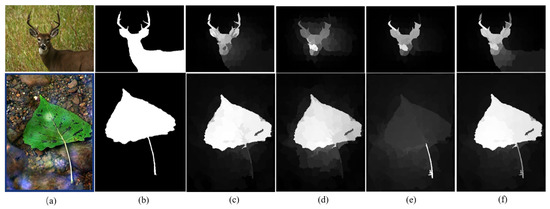
Figure 1.
A glimpse of different methods: (a) input images; (b) ground truth; (c) saliency maps using the MFMR method [18] based on color features; (d) saliency maps using the method based on low-level features; (e) saliency maps using the method based on high-level features; (f) our method.
Compared with bottom-up methods, deep learning methods have achieved a great level of performance [26,27,28,29]. Shen et al. [30] used sparse noise to represent the object regions, and the low-rank matrix represented the background regions. To achieve better performance, high-level features were incorporated to produce prior maps. Li et al. [31] extracted high-level features from a deep convolutional neural network (CNN) at three different scales. The high-level feature maps and spatial consistency model were applied to each multi-level segmentation. Thus, the refined salient maps were fused into a final salient map. Zhao et al. [32] proposed a deep learning method based on a multi-context with both local features and context. Girshick et al. [33] applied a convolutional neural network to the bottom-up model to locate and segment the objects.
Deep neural networks facilitate the learning of complex high-level features and models. Deep features can discriminate objects in an image while having difficulty locating the precise boundary of the objects. As evident in Figure 1, the saliency maps using only deep features are not ideal for locating objects precisely.
It is not optimal to use hand-crafted features or deep features alone in saliency detection, but they have their own advantages and can complementarily represent the images. Deep features can evaluate the coarse spatial location of the object in an image. The latter layers of deep features are weak in detecting the boundaries of objects and background regions but are closely related to the classification of semantics. Meanwhile, we can evaluate the similarities in appearance between the different image patches relying on low-level features. The aim of saliency detection is to segment foregrounds from backgrounds precisely rather than to identify their classification of semantics. Thus, in this paper, on the basis of [18], we incorporated the semantic deep features extracted from a CNN as well as hand-crafted features in an unsupervised way, and a ranking method in manifold space helped to construct final saliency maps.
In summary, our method has three main contributions: (1) We propose an efficient multi-feature manifold ranking algorithm to detect salient objects. We used a feature vector including the low-level features and high-level features of input images to represent the image regions, which can better capture object regions when conventional saliency detection may fail. (2) On the new feature vector, we utilized the complementary relationship of multi-features to further refine the detection results. Moreover, the saliency maps were formed with the manifold space-ranking method. (3) Our empirical experiments show that our method achieves better results in terms of evaluation metrics against comparative state-of-the-art methods.
2. Related Work
Graph-Based Manifold Ranking
Based on the method of [17], we suppose an input image contains n regions , and the n regions are disconnected sets. We select some regions as marked seeds, and the other regions are sorted based on their relevance to the query seeds. The graph-based method should first compute the affinities of all the regions by constructing an affinity matrix. The affinity matrix is an important process for obtaining a higher detection effect. Given the affinity matrix W, and denoted by weight between different nodes i and j,
where = 0 to avoid self-reinforcement, and are extracted features, and is a coefficient for restricting the weight.
The ranking method can be regarded as a manifold structure [22]. Given f represents a sorting score by a sorting function, denoted by a vector . Suppose , when is a query seed, let , and set is 0 when is not a query seed. After that, an indication graph is constructed, in which V represents the n regions and edge E is defined by affinity matrix W. Thus, we obtain the ranking results by solving optimization problems by Equation (2):
where represents the ranking results, and is a balancing constant. We have the ranking function by setting the derivative of Equation (2) to zero [17]:
where I represents an identity matrix. Set =1/(1+) and S= is the normalized Laplacian matrix. The degree matrix , . Thus, Equation (3) turns into [17]:
3. The Proposed Method
Our method has three steps. First, we extracted the low- and high-level features from deep neural networks to measure the similarity of different image patches. Then, the saliency of image patches was computed in manifold space based on prior boundaries. Finally, we fused four coarse saliency maps to produce the final results. The overview of our method is depicted in Figure 2.
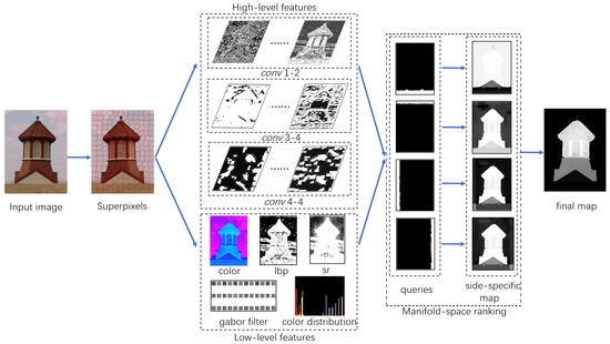
Figure 2.
Overall pipeline of our method, including feature extraction, manifold space ranking, and the final saliency map.
We first used the efficient SLIC algorithm [34] to segment the image into irregular regions. An irregular region consists of pixels that have adjacent and similar features such as texture, color, and brightness. Each region is regarded as a superpixel or a node. In this paper, the extraction of multi-features was performed on each node, and the multi-features helped to capture more information (compared with color features) of each node.
3.1. Low-Level Feature Extraction
We extracted five different visual features that are the most common visual features to represent each superpixel:
Mean color. The mean color feature is the average color of all the pixels in each superpixel, which was extracted in the CIELab color space. This yields three color features;
Color histogram. The values of color histograms are all statistics, which describe the statistical distribution and basic hue of the colors in an image. In the CIELab color space, we quantized the number of L channels as 16 bins, the number of a channel as 8 bins, and the number of b channel as 8 bins. This yielded 16 + 8 + 8 = 32 color features;
Gabor filters. Gabor filters as bandpass filters are preprocessing steps for extracting features and analyzing textures. The product of complex oscillation and the Gaussian envelope function generates the impulse response of these filters. We extracted the Gabor filter responses in 12 directions and 3 scales. The minimum filter bandwidth was set to 3, the scaling factor was set to 2, and the ratio of the Gaussian function representing the standard deviation in the propagation function to the center frequency of the Gabor filter was set to 0.65. This yielded 12 × 3 = 36 features;
Local binary pattern (LBP) [35]. Lbp is one of the texture features and is invariant to light, which was computed by the differences between a pixel and its neighborhoods. This yielded one feature;
Spectral residual. Spectral residual used each color channel separately. Fourier transformed was run on an image, which weakened the magnitude components. The frequency distribution was then converted into a gray distribution using the inverse Fourier transform conversion. This yielded one feature.
After we extracted the low-level features, we combined these 73 features into a feature vector.
3.2. High-Level Feature Extraction
Low-level features can measure the difference between each node by image appearance. In order to represent the image information more comprehensively, high-level features have been used in image-processing tasks. Recently, saliency detection methods based on CNNs have achieved superior performance [36,37]. Thus, we exploited the pretrained VGGNet-19 [36] to extract semantic information from an image. The semantic classification between objects and background is strengthened and spatial resolution is gradually reduced when features are propagated to deeper layers. On the other hand, the earlier layers of VGGNet-19 show higher spatial resolution for the precise localization of the objects. For saliency detection, we focused more on the accurate locations of objects than their semantic category. We thus employed the semantic classification of the latter layers to discriminate obvious category differences from the background and used the information of earlier layers to fix the precise localization of the objects. We visualized the upsampled outputs of the 1-2, 2-2, 3-4, 4-4, and 5-4 convolutional layers (Figure 3). As shown in Figure 3, the 1-2 layer has more precise localization information similar to a hand-crafted low-level feature map, the 3-4 and 4-4 layers show large appearance changes, and the 5-4 layer is not good at locating the contour of the objects due to its coarse spatial resolution [36]. There are two reasons for using a pretrained CNN. First of all, since pretrained CNNs do not require adjusting the net, it becomes easier and more convenient to extract deep features. Secondly, since the pretrained CNN model was trained from 1000 classified images, these can help to recognize an unknown object well with model-free identification [36]. In this paper, we exploited the responses from the 1-2, 3-4, and 4-4 layers as image representations. The number of features for 1-2, 3-4, and 4-4 was 64, 256, and 512, respectively. Deep image features as well as hand-crafted features were incorporated into a new image feature space to evaluate the difference in image patches. The new feature vector is summarized in Table 1. Considering computational efficiency, we used the PCA (principal component analysis) algorithm [38] to eliminate redundant information. After that, the image feature vector was reduced by using fewer principal components.
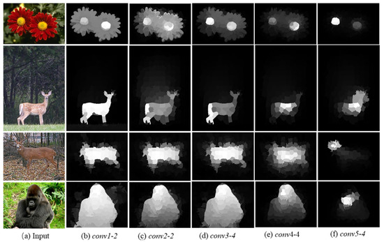
Figure 3.
Visualization of convolutional layers: (a) input images from the ECSSD dataset; (b–f) saliency maps from the outputs of the convolutional layers 1-2, 2-2, 3-4, 4-4, and 5-4 using the VGGNet-19 [36].

Table 1.
The dimension of feature vectors.
Our method does not need to train many images, so it is easier to obtain the features of nodes. In order to show the effect of the new feature vector on the saliency detection task more intuitively, we exploited several methods based on different features to detect the same objects. The results are shown in Figure 1. The MFMR [18] method is based on color features, Figure 1d is our proposed method based on only low-level features, and Figure 1e is our proposed method based on only high-level features. We can note that our method detected the saliency objects better than any method using a single feature.
3.3. Saliency Detection in Two Stages
3.3.1. Ranking with Background Seeds
We extracted the multi-features of each node to form a new feature vector. The distance between the two nodes in Equation (1) can be measured using this new feature vector. It is commonly known that the background region and boundary regions often have similarities in appearance [17,39]. That is, the salient objects are relatively uniform in structure and have spatial distribution, and the affinity matrix [17] can also infer these. Many previous saliency detection methods have applied the prior boundary method, and it is more effective than the prior center method [1,5]. In this paper, we also used boundary regions as background queries. The nodes in the four boundary regions of the image were first marked as background seeds. The saliency values of other nodes were computed by their relevance to the background seeds. Specifically, we used prior boundaries to obtain four saliency maps and then fused them into coarse saliency maps, as shown in Figure 2. The fusion Equation [17] is
where the saliency maps , , , and are generated by using the top boundary, the bottom boundary, the left boundary, and the right boundary as background seeds, respectively.
3.3.2. Ranking with Foreground Seeds
We obtained the coarse saliency map obtained by the above steps, but the saliency map did not uniformly highlight the saliency objects. Thus, we continued to binarize the map using the mean saliency over the entire saliency map and selected the foreground nodes as query seeds. The ranking value can be defined by Equation (4). is normalized between 0 and 1, and the final saliency map [17] is produced as follows:
where denotes the normalized vector of superpixel i.
4. Experimental Validation and Analysis
In order to evaluate the performance of our algorithm, we measured the proposed algorithm on four different datasets, namely MSRA-5000, DUT-OMRON, SOD, and ECSSD. MSRA-5000 contains 5000 natural images, and the background regions of the images are complex. DUT-OMRON includes 5168 high-quality challenging images in which backgrounds and objects are more comprehensive. SOD contains 300 images, and some of their salient objects are close to the boundary of the images. It is a very challenging image dataset. ECSSD includes 1000 semantic meaning images with multiple objects. All images have their corresponding ground truth images in the above four datasets.
We visually and quantitatively compared our approach with 14 previous detection algorithms, including AC (2015) [40], SR (2014) [27], MSS (2010) [41], GBVS (2006) [42], WTLL (2013) [43], LRMR (2012) [30], MR (2013) [17], BMA (2019) [44], FT (2009) [24], BFSS (2015) [15], GR (2013) [45], SWD (2011) [46], RR (2015) [39], and MFMR (2021) [18]. We tested these methods with MATLAB 2016. The CPU is 3.60 GHz CPU, and RAM is 64 GB.
4.1. Experiment Setup
Since most of the images have a resolution of 300 × 400 pixels in the four datasets, we segmented each image into 200 superpixels to balance the efficiency and accuracy of the calculation by reference to previous works [15,17]. In Equations (3) and (4), the coefficient of the affinity matrix was set to 0.99, similar to a previous study [17]. In Equation (1), the parameter was set to 0.1 [17].
4.2. Visual Performance Comparison
Some detection results produced by our model and compared methods are shown in Figure 4. In addition to our method, the results of other methods are from our previous paper [18]. We note that the AC, SR, MSS, and FT methods fully detect the whole object regions, but the contrast with the background is low. The GBVS, BMA, and SWD methods can detect saliency objects roughly, but the object regions are blurred and uneven. The WTLL and LRMR methods find out the regions with special pixels, but the edge of saliency regions is not clear. The MR, GR, RR, and MFMR methods highlight the edge of the saliency regions, but their detection results are not complete when multiple objects appear in the image. The BFSS method can detect the region with high color contrast, but it erroneously identifies background areas as the foreground areas. Our method exhibits superior performance, especially in challenging scenes. For instance, when the input image is low contrast, as shown in Figure 4(h), the other compared methods are not able to detect the objects accurately, while our method, benefiting from the multi-feature component, is still closest to the ground truth.
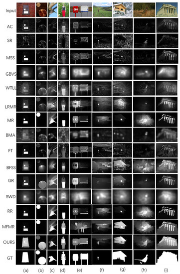
Figure 4.
Visual comparisons of different methods on four datasets: (a–c) MSRA-5000 dataset; (d,e) ECSSD dataset; (f,g) SOD dataset; (h,i) DUT-OMRON dataset.
4.3. Quantitative Performance Comparison
We used precision–recall curves, ROC curves, and F-measure bar graphs to evaluate our method and other compared models. The results are reported in Figure 5, Figure 6 and Figure 7. We compared our algorithm with other algorithms in terms of the scores of precision, recall, AUC, and F-measure, as listed in Table 2. The graphs and table of other compared methods are from our previous paper [18].
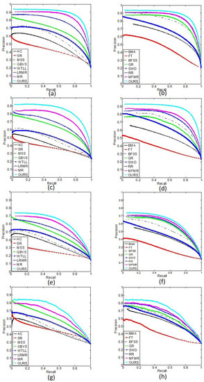
Figure 5.
The PR curves of different methods on four datasets: (a,b) MSRA-5000 dataset; (c,d) ECSSD dataset; (e,f) DUT-OMRON dataset; (g,h) SOD dataset.
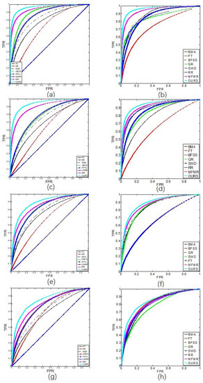
Figure 6.
The ROC curves of different methods on four datasets: (a,b) MSRA-5000 dataset; (c,d) ECSSD dataset; (e,f) DUT-OMRON dataset; (g,h) SOD dataset.
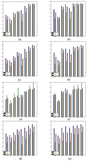
Figure 7.
The average precision, recall and F-measure scores of different methods: (a,b) MSRA-5000 dataset; (c,d) ECSSD dataset; (e,f) DUT-OMRON dataset; (g,h) SOD dataset.
Table 2.
Evaluation metrics of different methods in four datasets.
It can be noted that our model not only shows satisfactory results for the four datasets under all evaluation curves but also outperforms the compared methods with dominant advantages. This is due to having multi-feature, as the saliency objects are better segmented from backgrounds. In Table 2, we note that for the methods whose precision values are comparable to our method (i.e., MFMR, GR), their values of recall and F-measure are often much lower on MSRA-5000 and DUT-OMRON datasets. Thus, they are more likely to miss some salient information. In the ECSSD dataset, our model achieves 81.08% precision and 72.29% recall, while the second-best model (MFMR) achieves 78.29% precision and 67.70% recall. The improvement in the performance of our method is due to its multi-feature extraction. The new feature vector composed of multi-feature shows its complementary advantages and achieves better results.
4.4. Limitation and Analysis
In Figure 8, we present a failure case with our method. When the color contrast of the object region and the background region is very low, our method fails to detect the whole object. This is because different features are often good at different aspects of an image. The features are directly concatenated and may not completely represent complementary information of different features. In the existing methods, even deep-learning-based methods, saliency detection is also a challenge for low-contrast images. Thus, We look forward to improving the detection method for low-contrast images from a multi-view perspective in our future research.
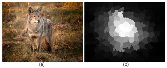
Figure 8.
Failure result of our method: (a) input image; (b) saliency map of our method.
5. Conclusions
We proposed a saliency detection method based on multiple features via manifold space ranking. The semantically rich deep features derived from a CNN model (VGG19) help to accurately distinguish between objects and backgrounds but fail to fix the precise localization of the objects. Hand-crafted low-level features have a strong discriminative function to measure the similarity between different image regions. Considering the different roles of these two features, we exploited both complementary features to describe image patches. Furthermore, we adopted a manifold space-ranking method to rank the saliency of the image patches. Without any preprocessing and postprocessing, our method achieved superior performance with the help of multi-feature.
Author Contributions
Conceptualization, X.L. and Y.L.; methodology, X.L. and Y.L.; software, Y.L.; validation, X.L., Y.L. and H.Z.; formal analysis, H.Z.; investigation, X.L.; resources, Y.L.; data curation, X.L.; writing—original draft preparation, X.L. and Y.L.; writing—review and editing, X.L.; visualization, X.L.; supervision, Y.L.; project administration, Y.L.; funding acquisition, Y.L. All authors have read and agreed to the published version of the manuscript.
Funding
This research was supported by the Science and Technology Innovation Key Fund project of the Chinese Academy of Sciences grant Y8K4160401.
Data Availability Statement
Not applicable.
Conflicts of Interest
The authors declare no conflict of interest.
References
- Mahadevan, V.; Vasconcelos, N. Saliency-based discriminant tracking. In Proceedings of the Computer Vision and Pattern Recognition, Miami, FL, USA, 20–25 June 2009; pp. 1007–1013. [Google Scholar]
- Ding, Y.; Xiao, J.; Yu, J. Importance filtering for image retargeting. In Proceedings of the Computer Vision and Pattern Recognition, Colorado Springs, CO, USA, 20–25 June 2011; pp. 89–96. [Google Scholar]
- Sun, J.; Ling, H. Scale and object aware image retargeting for thumbnail browsing. In Proceedings of the 2011 International Conference on Computer Vision, Barcelona, Spain, 11–14 November 2011; pp. 1511–1518. [Google Scholar]
- Han, S.; Vasconcelos, N. Biologically plausible salicency mechanisms improve feedforward object recognition. Vis. Res. 2010, 50, 2295–2307. [Google Scholar] [CrossRef] [PubMed]
- Ishikura, K.; Kurita, N.; Chandler, D.M.; Ohashi, G. Saliency detection based on multiscale extrema of local perceptual color differences. IEEE Trans. Image Process. 2018, 27, 703–717. [Google Scholar] [CrossRef]
- Wang, L.; Xue, J.; Zheng, N.; Hua, G. Automatic salient object extraction with contextual cue. In Proceedings of the 2011 International Conference on Computer Vision, Barcelona, Spain, 11–14 November 2011; pp. 105–112. [Google Scholar]
- Lempitsky, V.; Kohli, P.; Rother, C.; Sharp, T. Image segmentation with a bounding box prior. In Proceedings of the 2009 IEEE 12th International Conference on Computer Vision, Kyoto, Japan, 27 September–4 October 2009; pp. 277–284. [Google Scholar]
- Itti, L.; Koch, C.; Niebur, E. A model of saliency-based visual attention for rapid scene analysis. IEEE Trans. Pattern Anal. Mach. Intell. 1998, 20, 1254–1259. [Google Scholar] [CrossRef]
- Judd, T.; Ehinger, F.; Torralba, A. Learning to predict where humans look. In Proceedings of the 6th International Conference on Computer Vision, Tokyo, Japan, 27 September–4 October 2009; pp. 2106–2113. [Google Scholar]
- Liu, T.; Yuan, Z.J.; Sun, J.; Wang, J.D.; Zheng, N.N.; Tang, X.O.; Shum, H.Y. Learning to Detect a Salient Object. IEEE Trans. Pattern Anal. Mach. Intell. 2011, 33, 353–367. [Google Scholar] [PubMed]
- Goferman, S.; Zelnik-Manor, L.; Tal, A. Context-aware saliency detection. In Proceedings of the Computer Vision and Pattern Recognition, San Francisco, CA, USA, 13–18 June 2010; pp. 1915–1926. [Google Scholar]
- Cheng, M.M.; Mitra, N.; Huang, X.; Torr, P.; Hu, S. Global contrast based salient region detection. IEEE Trans. Pattern Anal. Mach. Intell. 2015, 37, 569–582. [Google Scholar] [CrossRef] [PubMed]
- Shi, J.P.; Yan, Q.; Xu, L.; Jia, J. Hierarchical Image Saliency Detection on Extended CSSD. IEEE Trans. Pattern Anal. Mach. Intell. 2016, 38, 717–729. [Google Scholar] [CrossRef] [PubMed]
- Zhu, W.J.; Liang, S.; Wei, Y.C.; Sun, J. Saliency optimization from robust background detection. In Proceedings of the Computer Vision and Pattern Recognition, Columbus, OH, USA, 24–29 June 2014; pp. 2814–2821. [Google Scholar]
- Wang, J.P.; Lu, H.C.; Li, X.H.; Tong, N.; Liu, W. Saliency detection via background and foreground seed selection. Neurocomputing 2015, 152, 359–368. [Google Scholar] [CrossRef]
- Wei, Y.; Wen, W.; Sun, J.A. Geodesic saliency using background priors. In Proceedings of the European Conference on Computer Vision, Firenze, Italy, 7–13 October 2012; pp. 29–42. [Google Scholar]
- Yang, C.; Zhang, L.; Lu, H.C.; Ruan, X.; Yang, M. Saliency Detection via Graph-Based Manifold Ranking. In Proceedings of the Computer Vision and Pattern Recognition, Portland, OR, USA, 23–28 June 2013; pp. 3166–3173. [Google Scholar]
- Li, X.L.; Liu, Y.P.; Zhao, H.C. Image Saliency Detection via Multi-Feature and manifold-Space Ranking. In Proceedings of the Asia Pacific Information Technology, Bangkok, Thailand, 15–17 January 2021; pp. 76–81. [Google Scholar]
- Deng, C.; Liu, X.; Li, C.; Tao, D. Active multi-kernel domain adaptation for hyperspectral image classification. Pattern Recognit. 2018, 77, 306–315. [Google Scholar] [CrossRef]
- Yang, M.L.; Deng, C.; Nie, F.P. Adaptive-weighting discriminative regression for multi-view classification. Pattern Recognit. 2019, 88, 236–245. [Google Scholar] [CrossRef]
- Wang, M.; Konrad, J.; Ishwar, P.; Jing, K.; Rowley, H. Image saliency: From intrinsic to extrinsic context. In Proceedings of the Computer Vision and Pattern Recognition, Colorado Springs, CO, USA, 20–25 June 2011; pp. 417–424. [Google Scholar]
- Zhang, L.; Yang, C.; Lu, H.; Ruan, X.; Yang, M.H. Ranking saliency. Pattern Anal. Mach. Intell. 2017, 39, 1892–1904. [Google Scholar] [CrossRef] [PubMed]
- Deng, C.; Nie, F.; Tao, D. Saliency detection via a multiple self-weighted graph-based manifold ranking. Multimedia 2020, 22, 885–896. [Google Scholar] [CrossRef]
- Achanta, R.; Hemami, S.; Estrada, F.; Susstrunk, S. Frequency-tuned salient region detection. In Proceedings of the Computer Vision and Pattern Recognition, Miami, FL, USA, 20–25 June 2009; pp. 1597–1604. [Google Scholar]
- Hou, X.D.; Zhang, L.Q. Saliency Detection: A Spectral Residual Approach. In Proceedings of the Computer Vision and Pattern Recognition, Minneapolis, MN, USA, 19–23 June 2007; pp. 1–8. [Google Scholar]
- Hou, Q.B.; Cheng, M.M.; Hu, X.W.; Borji, A.; Tu, Z.W.; Torr, P. Deeply supervised salient object detection with short connections. IEEE Trans. Pattern Anal. Mach. Intell. 2018, 41, 815–828. [Google Scholar] [CrossRef] [PubMed]
- Zhang, P.P.; Wang, D.; Lu, H.C.; Wang, H.Y.; Ruan, X. Amulet: Aggregating Multi-level Convolutional Features for Salient Object Detection. In Proceedings of the 2017 IEEE International Conference on Computer Vision, Venice, Italy, 22–29 October 2017; pp. 202–211. [Google Scholar]
- Wang, T.T.; Zhang, L.H.; Wang, S.; Lu, H.; Yang, G.; Ruan, X.; Borji, A. Detect globally, refine locally: A novel approach to saliency detection. In Proceedings of the Computer Vision and Pattern Recognition, Salt Lake City, UT, USA, 19–22 June 2018; pp. 3127–3135. [Google Scholar]
- Zhang, X.N.; Wang, T.T.; Qi, J.Q.; Lu, H.C.; Wang, G. Progressive Attention Guided Recurrent Network for Salient Object Detection. In Proceedings of the Computer Vision and Pattern Recognition, Salt Lake City, UT, USA, 19–22 June 2018; pp. 714–722. [Google Scholar]
- Shen, X.H.; Wu, Y. A Unified Approach to Salient Object Detection via Low Rank Matrix Recovery. In Proceedings of the Computer Vision and Pattern Recognition, Providence, RI, USA, 16–21 June 2012; pp. 853–860. [Google Scholar]
- Li, G.B.; Yu, Y.Z. Visual saliency based on multiscale deep features. In Proceedings of the Computer Vision and Pattern Recognition, Boston, MA, USA, 8–10 June 2015; pp. 5455–5463. [Google Scholar]
- Zhao, R.; Ouyang, W.L.; Li, H.S.; Wang, X.G. Saliency detection by multi-context deep learning. In Proceedings of the Computer Vision and Pattern Recognition, Boston, MA, USA, 8–10 June 2015; pp. 1265–1274. [Google Scholar]
- Girshick, R.; Donahue, J.; Darrell, T.; Malik, J. Rich feature hierarchies for accurate object detection and semantic segmention. In Proceedings of the Computer Vision and Pattern Recognition, Columbus, OH, USA, 23–28 June 2014; pp. 5455–5463. [Google Scholar]
- Achanta, R.; Shaji, A.; Smith, K.; Lucchi, A.; Fua, P.; Süsstrunk, S. Slic Superpixels; EPFL Scientific Publication: Lausanne, Switzerland, 2010. [Google Scholar]
- Ojala, T.; Pietikainen, M.; Maenpaa, T. Multiresolution gray-scale and rotation invariant texture classification with local binary patterns. IEEE Trans. Pattern Anal. Mach. Intell. 2002, 24, 71–987. [Google Scholar] [CrossRef]
- Ma, C.; Huang, J.B.; Yang, X.K.; Yang, M.H. Robust Visual Tracking via Hierarchical Convolutional Features. IEEE Trans. Pattern Anal. Mach. Intell. 2019, 41, 2709–2723. [Google Scholar] [CrossRef] [PubMed]
- Simonyan, K.; Zisserman, A. Very deep convolutional networks for large-scale image recognition. In Proceedings of the 3rd International Conference on Learning Representations, San Diego, CA, USA, 7–9 May 2015. [Google Scholar]
- Ganesh, R.N. Advances in Principal Component Analysis: Research and Development; Springer: Singapore, 2018. [Google Scholar]
- Li, C.Y.; Yuan, Y.C.; Cai, W.D.; Xia, Y.; Feng, D.D. Robust saliency detection via regularized random walks ranking. In Proceedings of the Computer Vision and Pattern Recognition, Boston, MA, USA, 8–10 June 2015; pp. 2710–2717. [Google Scholar]
- Achanta, R.; Estrada, F.; Wils, P.; Süsstrunk, S. Salient region detection and segmentation. In Proceedings of the 6th International Conference on Computer Vision systems, Santorini, Greece, 12–15 May 2008; pp. 66–75. [Google Scholar]
- Achanta, R.; Süsstrunk, S. Saliency detection using maximum symmetric surround. In Proceedings of the 2010 IEEE International Conference on Image Processing, Hong Kong, China, 26–28 September 2010; pp. 2653–2656. [Google Scholar]
- Harel, J.; Koch, C.; Perona, P.; Schölkopf, B.; Platt, J.; Hofmann, T. Graph-based visual saliency. In Proceedings of the 20th Annual Conference on Neural Information Processing Systems, Vancouver, BC, Canada, 4–7 December 2006; pp. 545–552. [Google Scholar]
- Lmamoglu, N.; Lin, W.; Fang, Y.M. A saliency detection model using low-level features based on wavelet. IEEE Trans. Multimed. 2013, 15, 96–105. [Google Scholar] [CrossRef]
- Zhang, J.M.; Sclaroff, S. Exploiting surroundedness for saliency detection: A boolean map approach. IEEE Trans. Pattern Anal. Mach. Intell. 2016, 38, 889–902. [Google Scholar] [CrossRef] [PubMed]
- Yang, C.; Zhang, L.H.; Lu, H.C. Graph-regularized Saliency Detection with Convex-hull-based Center Prior. IEEE Signal Process. Lett. 2013, 20, 637–640. [Google Scholar] [CrossRef]
- Duan, L.J.; Wu, C.P.; Miao, J.; Qing, L.Y.; Fu, Y. Visual saliency detection by spatially weighted dissimilarity. In Proceedings of the Computer Vision and Pattern Recognition, Colorado Springs, CO, USA, 20–25 June 2011; pp. 473–480. [Google Scholar]


Disclaimer/Publisher’s Note: The statements, opinions and data contained in all publications are solely those of the individual author(s) and contributor(s) and not of MDPI and/or the editor(s). MDPI and/or the editor(s) disclaim responsibility for any injury to people or property resulting from any ideas, methods, instructions or products referred to in the content. |
© 2023 by the authors. Licensee MDPI, Basel, Switzerland. This article is an open access article distributed under the terms and conditions of the Creative Commons Attribution (CC BY) license (https://creativecommons.org/licenses/by/4.0/).