Robot Manipulation Skills Transfer for Sim-to-Real in Unstructured Environments

Abstract

Robot force control that needs to be customized for the robot structure in unstructured environments with difficult-to-tune parameters guarantees robots’ compliance and safe human–robot interaction in an increasingly expanding work environment. Although reinforcement learning provides a new idea for the adaptive adjustment of these parameters, the policy often needs to be trained from scratch when used in new robotics, even in the same task. This paper proposes the episodic Natural Actor-Critic algorithm with action limits to improve robot admittance control and transfer motor skills between robots. The motion skills learned by simple simulated robots can be applied to complex real robots, reducing the difficulty of training and time consumption. The admittance control ensures the realizability and mobility of the robot’s compliance in all directions. At the same time, the reinforcement learning algorithm builds up the environment model and realizes the adaptive adjustment of the impedance parameters during the robot’s movement. In typical robot contact tasks, motor skills are trained in a robot with a simple structure in simulation and used for a robot with a complex structure in reality to perform the same task. The real robot’s performance in each task is similar to the simulated robot’s in the same environment, which verifies the method’s effectiveness.

1. Introduction

1.1. Motivations

Robots’ working scope has gradually expanded from factories to homes and even outdoors with the increased intelligence and structural complexity of robots. The tasks have also expanded from welding and painting, which only deal with workpieces, to human–robot interaction tasks such as artificial emotion, physical contact, and random tasks in unstructured environments [1,2,3]. However, traditional robots perform poorly on these new tasks. For example, robots based on position control often maintain a massive joint torque at the expense of high energy consumption to ensure position accuracy [4]. Although advances in the modeling and control of robot motors have made the position control of robot end-effector more accurate [5,6], the contact forces are also affected by the environment. The uncontrollable contact force may cause damage to the robot or fragile touched objects such as mirrors [7] or human bodies [8]. In addition to safety, contact force control, such as force tracking, has a wide range of applications, especially when the visual serving is inaccessible or the position of the object being touched is biased towards contact operations such as grasping, manufacturing, assembly and tool wear [9,10,11,12].

Although some robots have begun to use force control algorithms, the parameters in these algorithms are often designed for specific robots and are kept constant. When the robot becomes worn out or damaged, or these algorithms are redeployed on a new robot, the controller parameters need to be manually re-tuned The process is complicated, and the parameters are difficult to adjust to the optimum. Therefore, autonomous learning, improving and transferring robot motor skills are essential in complex or unknown environments [13].

Through accumulated experience in childhood and youth, the human nervous system has long been familiar with the force control of arm muscles [14], which brings new ideas to robot adaptive force control [15]. Therefore, the adaptive impedance control algorithm imitating the human learning skill has a broad application prospect and can significantly expand the application field of the robot. Unlike other intelligent algorithms that use static samples for cyclic training, reinforcement learning emphasizes the continuous interaction between the agent and the environment. The agent’s behavior is adjusted through rewards until the policy becomes optimal [16], which is more in line with the objective laws of the human learning process. Reinforcement learning can provide an alternative solution for robot control in structured environments and accomplish tasks that are difficult for classical control in unstructured environments.

1.2. Literature Overview

There has been much adaptive impedance based on classical control theory. Seul Jung et al. [17] used adaptive robust impedance control to solve the problem of constant force control in imprecise environments and robot models. However, this method only guarantees compliance in one direction. In recent years, many researchers have developed a series of reinforcement learning algorithms that can be applied to high-dimensional continuous state spaces. Jan Peters et al. [18] introduced the Fisher information metric into the Actor-Critic algorithm, used the natural gradient to update the Actor part, and obtained the NAC algorithm. Byungchan Kim et al. [19] improved the algorithm for adjusting the robot’s impedance online in uncoupled, weakly coupled, and strongly coupled contact tasks. However, robot torque control used in their method is usually inaccessible in most industrial robots. Cristian C. Beltran-Hernandez et al. [20] optimized the impedance parameters and the desired trajectory with the SAC algorithm [21]. However, the performance is susceptible to hyperparameters and cannot transfer between robots.

Since most industrial robots’ position controllers have been developed and have high control accuracy, instead of impedance control, admittance control is chosen in this paper to make the robot compliant with the environment in all directions. The admittance controller abstracts the robot into a second-order system with customizable impedance characteristics, ignoring the specific dynamics of the robot system, and thus can be transferred between robots with different structures. Hence, it is more reasonable to use the information in Cartesian space to adjust the impedance parameters. Training the agent based on the above information can also decouple the robot model from the environment model, and the agent can implicitly learn the environment model. In this paper, the eNAC algorithm [19] is modified and trains the agent on a simulated two-link robot with information under the Cartesian space to obtain the optimal policy. Optimal results are transferred to the KUKA IIWA robot on the same contact task with the unstructured environment where the KUKA IIWA robot achieves a competitive performance compared to the original robot, verifying the methods’ effectiveness.

1.3. Contributions and Organization

Here we list this paper’s actual contributions and organization in subsequent sections.

The contributions of our work are summarized as follows. (1) We design an online impedance adjustment scheme based on reinforcement learning that can be applied to real robots to improve the adaptability of robot compliance; (2) The mean and standard deviation of the action are explicitly set to vary in a range with an artificial neuron, avoiding the clipping operations for introducing range restrictions and ensuring the differentiability; (3) We propose methods to migrate the obtained motion skills from robots with simple structures in simulation to robots with complex structures in reality so that the policy does not need to be trained from scratch.

The remainder of this paper is organized as follows: Section 1 explains the problem. In Section 2, after comparing with other force control methods, admittance control is embodied in specific parts and implemented. The eNAC algorithm is improved and combined with the admittance control in Section 3. Finally, several contact tasks are analyzed and performed in Section 4. The conclusion is discussed in Section 5.

2. Robot Admittance Control

The ability to handle the robot’s physical contact with the environment is fundamental to the success of robotic contact tasks [4]. In these tasks, the environment and the robot model constantly interact, imposing various time-varying constraints on the robot’s motion. The gap between the actual robot and the robot model obtained at the beginning of the design gradually widened over time, while the environmental model is challenging to estimate or even completely unknown. Therefore, the compliance and safety of the robot is a vital improvement goal to ensure the successful execution of the robot contact task under a lack of accurate models.

The impedance control algorithm treats the robot as a spring system, which combines the force and displacement of the robot’s end effector. The generalized impedance control includes the position-based and force-based impedance control shown in Figure 1. The position-based impedance control is also called the admittance control.

The impedance controller transmits the force control signal to the robot system, while the admittance controller outputs the position control signal, where the robot system can be regarded as an impedance. The admittance control includes an inner position control loop and an outer force control loop. The external force controller generates position correction through contact force feedback and adjusts the input of the internal position control loop. In contrast, the internal position controller ensures that the robot moves along the input trajectory.

Therefore, by concretizing the control loop, we obtain Figure 2, which includes five parts: trajectory planning, robot motion controller, admittance controller, robot system, and environment. The purpose of trajectory planning is not to make the robot move strictly according to its generated trajectory but to ensure its interaction with the environment. The choice of position controller depends on the availability of the precise dynamics model.

2.1. Admittance Controller

The main idea of admittance control adopted in this paper is to generate a correction amount ${\mathbf{x}}_{\mathrm{dc}}$ in Cartesian space for the trajectory ${\mathbf{x}}_{\mathrm{d}}$ with the contact force ${\mathbf{F}}_{\mathrm{ext}}$ between the robot and the environment, so that the actual input of the motion controller is ${\mathbf{x}}_{\mathrm{c}}={\mathbf{x}}_{\mathrm{d}}-{\mathbf{x}}_{\mathrm{dc}}$ [22].

$${\mathbf{M}}_{\mathrm{d}}{\ddot{\mathbf{x}}}_{\mathrm{dc}}+{\mathbf{B}}_{\mathrm{d}}{\dot{\mathbf{x}}}_{\mathrm{dc}}+{\mathbf{K}}_{\mathrm{d}}{\mathbf{x}}_{\mathrm{dc}}={\mathbf{F}}_{\mathrm{ext}}.$$

(1)

In the impedance control (1), ${\mathbf{M}}_{\mathrm{d}}$, ${\mathbf{B}}_{\mathrm{d}}$, and ${\mathbf{K}}_{\mathrm{d}}$ are the robot model’s equivalent inertia, damping, and stiffness parameters, respectively. Small ${\mathbf{K}}_{\mathrm{d}}$ is usually selected in a high stiffness environment, while large ${\mathbf{K}}_{\mathrm{d}}$ is often used in a soft environment.

Since the impedance controller abstracts the robot as a second-order system, ignoring the actual structure of the robot, the transfer of impedance parameters between different robots is guaranteed. Therefore, the impedance control problem of a complex mechanism can be transformed into a simple one, reducing the difficulty and time consumption of parameter adjustment and robot control.

2.2. Position Controller

When the precise dynamic model can be accessed online, the computed torque controller can decouple the nonlinear control system into a linear system by combining the dynamic compensation quantity. Otherwise, the single-joint position controller based on PID is easy to implement, and only the inverse kinematics model is required.

The computed torque control based on the PD controller shown in (2) obtains the torque vector ${\mathbf{F}}_{\mathrm{tor}}$ applied to each joint through the difference between the expected motion and the actual motion in the joint space. ${\mathbf{q}}_{\mathrm{d}}$ and ${\dot{\mathbf{q}}}_{\mathrm{d}}$ are the desired position and velocity vector in joint space, while $\mathbf{q}$ and $\dot{\mathbf{q}}$ are the corresponding items in the actual motion.

$${\mathbf{F}}_{\mathrm{tor}}=\mathbf{M}({\mathbf{k}}_{\mathrm{p}}({\mathbf{q}}_{\mathrm{d}}-\mathbf{q})+{\mathbf{k}}_{\mathrm{d}}({\dot{\mathbf{q}}}_{\mathrm{d}}-\dot{\mathbf{q}}))+\mathbf{C}+\mathbf{F}+\mathbf{G}+{{\mathbf{J}}_{\mathrm{r}}}^{\mathrm{T}}{\mathbf{F}}_{\mathrm{ext}}.$$

(2)

$\mathbf{M}$ is the inertia matrix of the robot model, $\mathbf{C}$ is the compensation of the Coriolis force and centrifugal force, $\mathbf{F}$ is the friction torque, $\mathbf{G}$ is the gravitational moment, the last item ${\mathbf{F}}_{\mathrm{ext}}$ gives the force and torque on the end effector, and ${\mathbf{J}}_{\mathrm{r}}$ is the geometric Jacobian matrix of the robot. ${\mathbf{k}}_{\mathrm{p}}$ and ${\mathbf{k}}_{\mathrm{d}}$ are robot PD controller parameters.

3. Reinforcement Learning

3.1. Fundamental Reinforcement Learning

As a sequential decision problem based on the Markov process, reinforcement learning mainly includes the agent and the environment [23]. At time t, the agent in status $\mathbf{s}$ in the state space $𝒮$ selects the action $\mathbf{a}$ in its action space $\mathcal{A}$ according to the policy $\pi$, thereby obtaining the reward value $r_t$ related to $\mathbf{s}$ and $\mathbf{s}$. Then the status transfers to the next one according to the state transition function. The agent’s goal is to obtain the maximum long-term return $\mathbf{J}$ in a period of $t\in \{0,1,2,\dots \}$.

Assuming that $\psi$ parameterizes the policy, with the policy ${\pi }_{\psi }$, the long-term discounted return obtained by the agent is shown in Equation (3). The discount rate $\gamma \in (0,1)$ can be regarded as the “foresight” of the algorithm and $d^{{\pi }_{\psi }}\left(\mathbf{s}\right)$ is called the discount state distribution.

$$\begin{array}{c}\hfill \mathbf{J}\left({\pi }_{\psi }\right)=\mathbf{J}\left(\psi \right)=E\left\{\sum _{k=0}^{\infty }{\gamma }^k{r}_k|{\mathbf{s}}_0,{\pi }_{\psi }\right\}=\underset{\mathcal{S}}{\int }{d}^{{\pi }_{\psi }}\left(\mathbf{s}\right)\underset{\mathcal{A}}{\int }{\pi }_{\psi }\left(\mathbf{a}|\mathbf{s}\right)r\left(\mathbf{s},\mathbf{a}\right)\mathrm{d}\mathbf{a}\mathrm{d}\mathbf{s}.\end{array}$$

(3)

Therefore, the goal can be transformed into using the derivative of the long-term discounted return with respect to the policy parameters $\psi$ to continuously update the parameters until parameters maximize $\mathbf{J}\left({\pi }_{\psi }\right)$, which is also the source of the idea of the policy gradient method. With the state-value function with initial state $\mathbf{s}$ in (4) and the action-value function with initial state-action pair $\left(\mathbf{s},\mathbf{a}\right)$ in (5), we can rewrite the long-term discounted return with initial state ${\mathbf{s}}_0$ and calculate its derivative with respect to the policy parameters in (6).

$$\begin{array}{c}\hfill {\mathbf{V}}^{{\pi }_{\psi }}\left(\mathbf{s}\right)=E\left\{\sum _{k=0}^{\infty }{\gamma }^k{r}_k|\mathbf{s},\pi \right\}\end{array}$$

(4)

$$\begin{array}{c}\hfill {\mathbf{Q}}^{{\pi }_{\psi }}(\mathbf{s},\mathbf{a})=E\left\{\sum _{k=0}^{\infty }{\gamma }^k{r}_k|\mathbf{s},\mathbf{a},\pi \right\}\end{array}$$

(5)

$$\begin{array}{cc}\hfill {\nabla }_{\psi }\mathbf{J}\left({\pi }_{\psi }\right)& ={\nabla }_{\psi }{\mathbf{V}}^{{\pi }_{\psi }}\left({\mathbf{s}}_0\right)\hfill \\ \hfill & =\underset{\mathcal{S}}{\int }{d}^{{\pi }_{\psi }}\left(\mathbf{s}\right)\underset{\mathcal{A}}{\int }{\nabla }_{\psi }{\pi }_{\psi }\left(\mathbf{a}|\mathbf{s}\right){\mathbf{Q}}^{{\pi }_{\psi }}\left(\mathbf{s},\mathbf{a}\right)\mathrm{d}\mathbf{a}\mathrm{d}\mathbf{s}\hfill \\ \hfill & =\underset{\mathcal{S}}{\int }{d}^{{\pi }_{\psi }}\left(\mathbf{s}\right)\underset{\mathcal{A}}{\int }{\pi }_{\psi }\left(\mathbf{a}|\mathbf{s}\right){\nabla }_{\psi }\log {\pi }_{\psi }(\mathbf{s},\mathbf{a}){\mathbf{A}}^{{\pi }_{\psi }}\left(\mathbf{s},\mathbf{a}\right)\mathrm{d}\mathbf{a}\mathrm{d}\mathbf{s}.\hfill \end{array}$$

(6)

The advantage function ${\mathbf{A}}^{{\pi }_{\psi }}\left(\mathbf{s},\mathbf{a}\right)$ in the last equation means the “advantage” of the reward brought by selecting the action $\mathbf{a}$ compared to the expected reward under the state $\mathbf{s}$. Therefore, the remaining problem is the estimation of the advantage function $\mathbf{A}$.

In reinforcement learning, the algorithm that combines the idea of the strategy gradient method and the value function method is called Actor-Critic method. As is shown in Figure 3, the actor part is responsible for selecting the action, while the critic is responsible for scoring the action. With the progress of training, the value function estimated by the Critic part becomes more and more accurate, and the policy improved by the Actor part according to the value function is also becoming better and better.

3.2. eNAC Method

A compatible approximator ${\mathbf{A}}_{\mathbf{w}}^{{\pi }_{\psi }}\left(\mathbf{s},\mathbf{a}\right)\approx {\nabla }_{\psi }\log {\pi }_{\psi }{\left(\mathbf{a}\right|\mathbf{s})}^{\mathrm{T}}\mathbf{w}$ [24] that is suitable for stochastic policies and produces unbiased estimates of the gradient is used in the eNAC algorithm [19], simplifying the gradient calculation to Equations (7) and (8).

$$\begin{array}{c}\hfill {\nabla }_{\psi }\mathbf{J}\left({\pi }_{\psi }\right)=\mathbf{F}\left(\psi \right)\mathbf{w}\end{array}$$

(7)

$$\begin{array}{c}\hfill \mathbf{F}\left(\psi \right)=\underset{\mathbf{S}}{\int }{d}^{{\pi }_{\psi }}\left(\mathbf{s}\right)\underset{\mathbf{A}}{\int }{\pi }_{\psi }\left(\mathbf{a}|\mathbf{s}\right){\nabla }_{\psi }\log {\pi }_{\psi }(\mathbf{s},\mathbf{a}){\nabla }_{\psi }\log {\pi }_{\psi }{(\mathbf{s},\mathbf{a})}^T\mathrm{d}\mathbf{a}\mathrm{d}\mathbf{s}.\end{array}$$

(8)

3.2.1. Natural Gradient in the Actor Section

When the policy parameters are multidimensional vectors with different element scales, it is not suitable to update the parameters with the same step size, so it is necessary to find a measure of the gap between the policy before and after the update. Considering that the essence of a parameter update is to update the policy, it is more reasonable to consider the generalized distance between the policies before and after the optimization. Kullback–Leibler divergence measures the closeness of two distributions well for policies in the form of probability distributions.

Therefore, the natural policy gradient method [18] based on the development of Kullback–Leibler divergence is considered, which can better reduce the influence of different parameter scales. The natural gradient direction is ${\tilde{\nabla }}_{\psi }\mathbf{J}\left(\psi \right)={\mathbf{G}}^{-1}\left(\psi \right){\nabla }_{\psi }\mathbf{J}\left(\psi \right)\approx {\mathbf{G}}^{-1}\left(\psi \right)\mathbf{F}\left(\psi \right)\mathbf{w}$, where $\mathbf{G}\left(\psi \right)$ is the Fisher Information Matrix. It can be proven that $\mathbf{F}\left(\psi \right)=\mathbf{G}\left(\psi \right)$ [18], so

$$\begin{array}{c}\hfill {\tilde{\nabla }}_{\psi }\mathbf{J}\left(\psi \right)\approx \mathbf{w}.\end{array}$$

(9)

Then, the parameter update rule can be written as (10). $\alpha$ stands for the learning rate.

$$\begin{array}{c}\hfill {\psi }_{t+1}={\psi }_t+\alpha \mathbf{w}.\end{array}$$

(10)

3.2.2. Advantage Function Estimation in the Critic Section

The remaining problem is the estimation of ${\mathbf{A}}_w^{{\pi }_{\psi }}(\mathbf{s},\mathbf{a})\approx {\nabla }_{\psi }\log {\pi }_{\psi }{\left(\mathbf{a}|\mathbf{s}\right)}^{\mathrm{T}}\mathbf{w}$ and the calculation of the gradient update $\mathbf{w}$. With the definition of the advantage function, we can get

$$\begin{array}{c}\hfill {\mathbf{A}}_{\mathbf{w}}^{{\pi }_{\psi }}({\mathbf{s}}_t,{\mathbf{a}}_t)\approx r_t+\gamma {\mathbf{V}}^{{\pi }_{\psi }}\left({\mathbf{s}}_{t+1}\right)-{\mathbf{V}}^{{\pi }_{\psi }}\left({\mathbf{s}}_t\right).\end{array}$$

(11)

For the $e\mathrm{N}$ episode, the weighted accumulation of (11) along time $t\in [1,N]$ gives

$$\begin{array}{cc}\hfill \sum _{t=0}^N{\gamma }^t{\mathbf{A}}_{\mathbf{w}}^{{\pi }_{\psi }}({\mathbf{s}}_t,{\mathbf{a}}_t)& \approx \sum _{t=0}^N{\gamma }^t{r}_t-\gamma {\mathbf{V}}^{{\pi }_{\psi }}({\mathbf{s}}_0)+{\gamma }^{N+1}{\mathbf{V}}^{{\pi }_{\psi }}({\mathbf{s}}_{N+1})\hfill \\ \hfill & \approx \sum _{t=0}^N{\gamma }^t{r}_t-\gamma {\mathbf{V}}^{{\pi }_{\psi }}({\mathbf{s}}_0)\hfill \end{array}$$

(12)

$$\begin{array}{c}\hfill \sum _{t=0}^N{\gamma }^t[{\nabla }_{\psi }\log {\pi }_{\psi }{\left(a\right|s)}^{\mathrm{T}},1]\left[\begin{array}{c}\mathbf{w}\\ v\end{array}\right]\approx \sum _{t=0}^N{\gamma }^t{r}_t\end{array}$$

(13)

$$\begin{array}{c}\hfill {{\tilde{\varphi }}^{\mathrm{T}}}_e\left[\begin{array}{c}\mathbf{w}\\ v\end{array}\right]={\tilde{r}}_e,\end{array}$$

(14)

where v compensates for ${\mathbf{V}}^{{\pi }_{\psi }}\left({\mathbf{s}}_0\right)$, and we have ${\tilde{\varphi }}_e^{\mathrm{T}}={\displaystyle \sum _{t=0}^N}{\gamma }^t[{\nabla }_{\psi }\log {\pi }_{\psi }{\left(\mathbf{a}\right|\mathbf{s})}^{\mathrm{T}},1]$, ${\tilde{r}}_e={\displaystyle \sum _{t=0}^N}{\gamma }^t{r}_t$. $\mathbf{w}$ can be calculated by combining (14) of different episodes and used in (10). A simple combination is the least squares method [25].

3.2.3. Stochastic Action Selection

Every action is generated by a Gaussian distribution with its mean $\mu$ and stand deviation $\sigma$ decided by the state in (15). ${\psi }_{*}^T$ and ${\eta }_{*}$ are the policy parameters while ${\xi }_1$ and ${\xi }_2$ are the scale factors of $\mu$ and $\sigma$, respectively.

$$\begin{array}{cc}\hfill \mu & ={\xi }_1(\mathrm{sigmoid}\left({\psi }_{*}^{\mathrm{T}}{\mathbf{s}}_t\right)-0.5)\hfill \\ \hfill \sigma & ={\xi }_2(\mathrm{sigmoid}\left({\eta }_{*}\right)+0.001).\hfill \end{array}$$

(15)

The mean $\mu$ is the scaled output with a bias value of $-0.5$ of a single artificial neuron with input ${\mathbf{s}}_t$ and parameter ${\psi }_{*}^T$. The activation function sigmoid limits the mean $\mu$ in the range $[-0.5{\xi }_1,0.5{\xi }_1]$, which not only ensures that the mean and the action will not change unrestricted due to the change of the state but also avoids the derivative calculation problem caused by the clip of the action. $\sigma$ is computed similarly and is restricted to the range $[0.001{\xi }_2,1.001{\xi }_2]$.

So, for the logarithmic derivative of the policy with respect to the parameter, we have

$$\begin{array}{cc}\hfill & {\nabla }_{{\theta }_{\mu }}\log \pi \left({\mathbf{a}}_t\right|{\mathbf{s}}_t)\hfill \\ \hfill & =\frac{{\mathbf{a}}_t-\mu }{{\sigma }^2}{\nabla }_{{\theta }_{\mu }}\mu \hfill \\ \hfill & ={\xi }_1\frac{{\mathbf{a}}_t-\mu }{{\sigma }^2}\mathrm{sigmoid}\left({\psi }_{*}^{\mathrm{T}}{\mathbf{s}}_t\right)(1-\mathrm{sigmoid}\left({\psi }_{*}^{\mathrm{T}}{\mathbf{s}}_t\right)){\mathbf{s}}_t\hfill \\ \hfill & {\nabla }_{{\theta }_{\sigma }}\log \pi \left({\mathbf{a}}_t\right|{\mathbf{s}}_t)\hfill \\ \hfill & =(\frac{{({\mathbf{a}}_t-\mu )}^2}{{\sigma }^3}-\frac{1}{\sigma }){\nabla }_{{\theta }_{\sigma }}\sigma \hfill \\ \hfill & ={\xi }_2(\frac{{({\mathbf{a}}_t-\mu )}^2}{{\sigma }^3}-\frac{1}{\sigma })\mathrm{sigmoid}\left({\eta }_{*}\right)(1-\mathrm{sigmoid}\left({\eta }_{*}\right)).\hfill \end{array}$$

(16)

3.2.4. Admittance Control Based on the eNAC Algorithm

Studies have shown that human arm control is similar to impedance control when performing contact tasks. The agonist and antagonist muscles are activated to contract together to adjust the arm impedance parameters, of which the stiffness parameter is the most significant [26].

Therefore, the robot’s movement in the Cartesian space and force information make up the state vector ${\mathbf{s}}_t$, and the action ${\mathbf{a}}_t$ determines the amount of change in the stiffness parameter ${\mathbf{K}}_{\mathrm{d}}$. The state’s composition and the action’s meaning vary between tasks. The stiffness is the function of the action. The contact force information can be combined with the position of the robot to infer the stiffness of the environment and with the robot’s speed to infer the environment’s damping. Since the state and action are not related to the specific configuration of the robot, the agent learns not the control method of a specific type of robot but the model of the environment and relies on the model to make decisions.

In summary, the primary process of the algorithm is shown in Algorithm 1.

Algorithm 1 Robot Admittance Control based on the eNAC Algorithm.

Input: initial training parameters, desired training episodes Output: policy parameter $\psi$  while interaction times < desired training episodes do   reset to initial state   repeat    generate action ${\mathbf{a}}_t$ according to policy $\pi$ and status ${\mathbf{s}}_t$    record reward $r_t$    update status: ${\mathbf{s}}_t\to {\mathbf{s}}_{t+1}$   until end of episode   if discounted reward qualifies then    Critic part: update $\mathbf{w}$ based on (14)    Actor part: update $\psi$ based on (10)   end if  end while

When tasks need to be performed on new robots, the learned results can be used differently. (1) The learned policy can adjust the robot’s stiffness online, and this method can ensure the continuation of the learning process; (2) The learned impedance parameter series can be directly used in the impedance controller of the new robot; (3) If the position control loop of the robot is accurate, the end-effector of the new robot can be directly controlled to move according to the trajectory of the end-effector of the old robot.

Since the optimal end-effector trajectory implicitly contains all the information of the environment model, when the environment remains unchanged, a more similar the trajectory will lead to a more similar contact force, ensuring the successful execution of the task. The remaining task is to adjust the installation position and posture of the new robot to ensure the end-effector trajectory execution within the limited range of joint angles. In addition, this method only requires the robot position controller, which can eliminate the need for expensive force sensors.

Collecting data from the actual robot with a complex structure is usually tricky and time-consuming. In contrast, the data acquisition of the robot in the simulation is fast and safe. The best solution is that the optimal trajectory is learned by the simple robot in the simulation and transmitted to the actual robot with a complex structure, namely sim-to-real. In this case, the computational complexity [27,28] that needs to be considered in the actual implementation is resolved, reducing the processor burden. The computational torque controller combined with dynamics can often achieve a good control effect for the simulated robot whose precise dynamics model is easy to obtain. For the actual robot whose dynamics model is challenging to obtain, the PID control of the independent joint combined with the inverse kinematics is easy to achieve.

4. Contact Task Experiments

This section selects two classical contact tasks to verify the method’s feasibility. The simulated robot was selected as a two-link robot in Figure 4, controlled by a computed torque controller. Its model and state can be obtained in real-time. The LBR IIWA 14 R820 from KUKA was selected as a physical robot and the robot motion controller provided by the Kuka sunrise toolbox [29] was selected as the single-joint PID controller for position control with inverse kinematics solved through the ROBOTICS TOOLBOX [30].

The robot’s links are identical, with a mass of $1\mathrm{kg}$ and a length of 0.5 m. The mass is concentrated at the end of the link. $\mathbf{M}$, $\mathbf{C}$, $\mathbf{G}$, ${\mathbf{J}}_{\mathbf{r}}$ in Equation (2) can be calculated through Equation (17). We ignore the joint friction so that all the terms in $\mathbf{F}$ are zero, and $\mathbf{G}$ is all zero when the robot is laid flat.

$$\begin{array}{cc}\hfill & \mathbf{M}=\left[\begin{array}{cc}{m}_1{l_1}^2+m_2{l_2}^2+m_2{l_1}^2+2m_2{l}_1{l}_2\cos \left(q_2\right)& m_2{l_2}^2+m_2{l}_1{l}_2\cos \left(q_2\right)\\ m_2{l_2}^2+m_2{l}_1{l}_2\cos \left(q_2\right)& m_2{l}_2^2\end{array}\right]\hfill \\ \hfill & \mathbf{C}=\left[\begin{array}{c}-m_2{l}_1{l}_2\sin \left(q_2\right){\dot{q}}_2^2-2m_2{l}_1{l}_2\sin \left(q_2\right){\dot{q}}_1{\dot{q}}_2\\ m_2{l}_1{l}_2\sin \left(q_2\right){\dot{q}}_1^2\end{array}\right]\hfill \\ \hfill & \mathbf{G}=\left[\begin{array}{c}(m_1{l}_1+m_2{l}_1)g\cos \left(q_1\right)+m_2{l}_{2}g\cos (q_1+q_2)\\ m_2{l}_{2}g\cos (q_1+q_2)\end{array}\right]\hfill \\ \hfill & {\mathbf{J}}_{\mathbf{r}}=\left[\begin{array}{c}{l}_1\cos \left(q_1\right)+l_2\cos (q1+q2)\\ l_1\sin \left(q_1\right)+l_2\sin (q1+q2).\end{array}\right]\hfill \end{array}$$

(17)

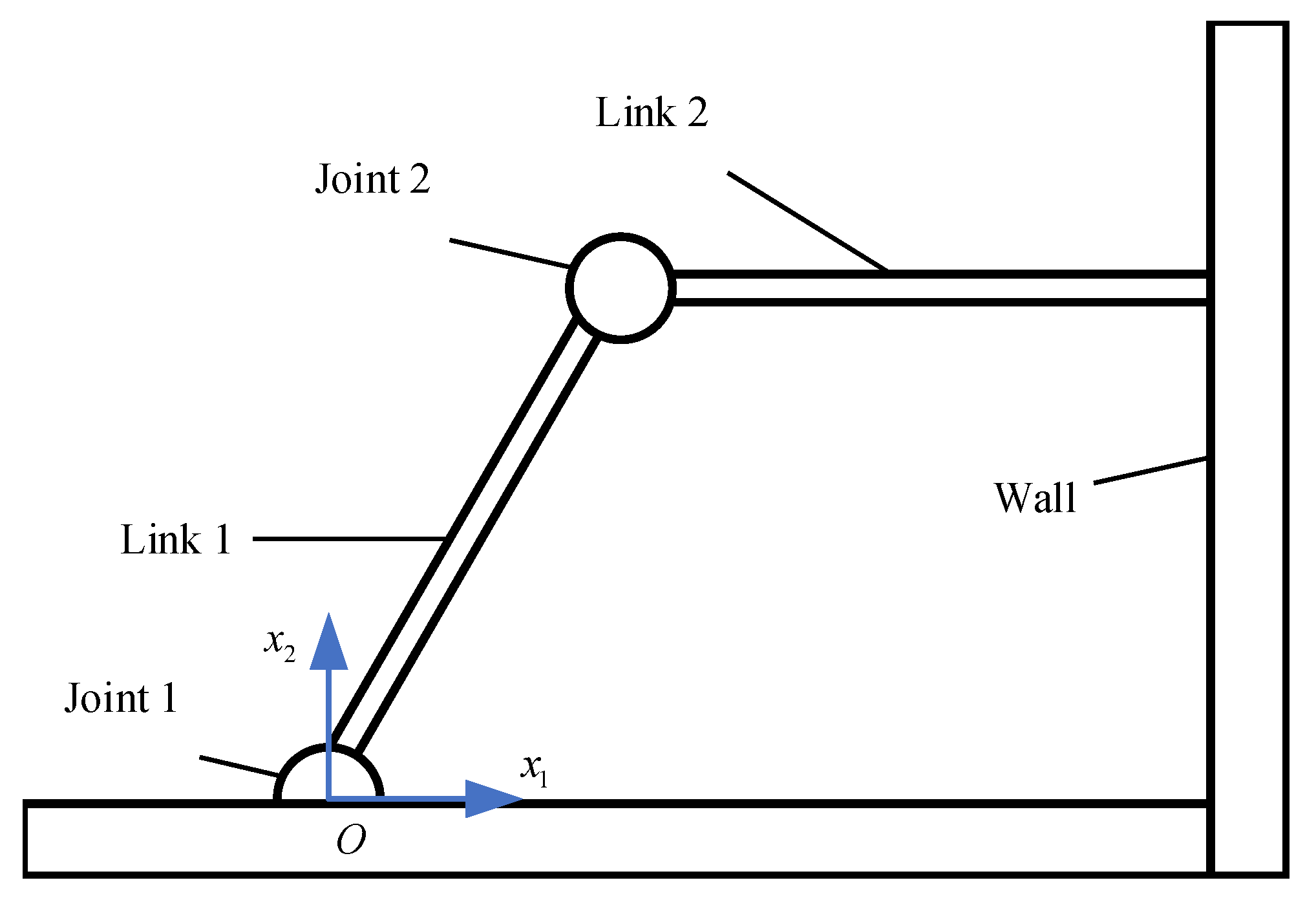
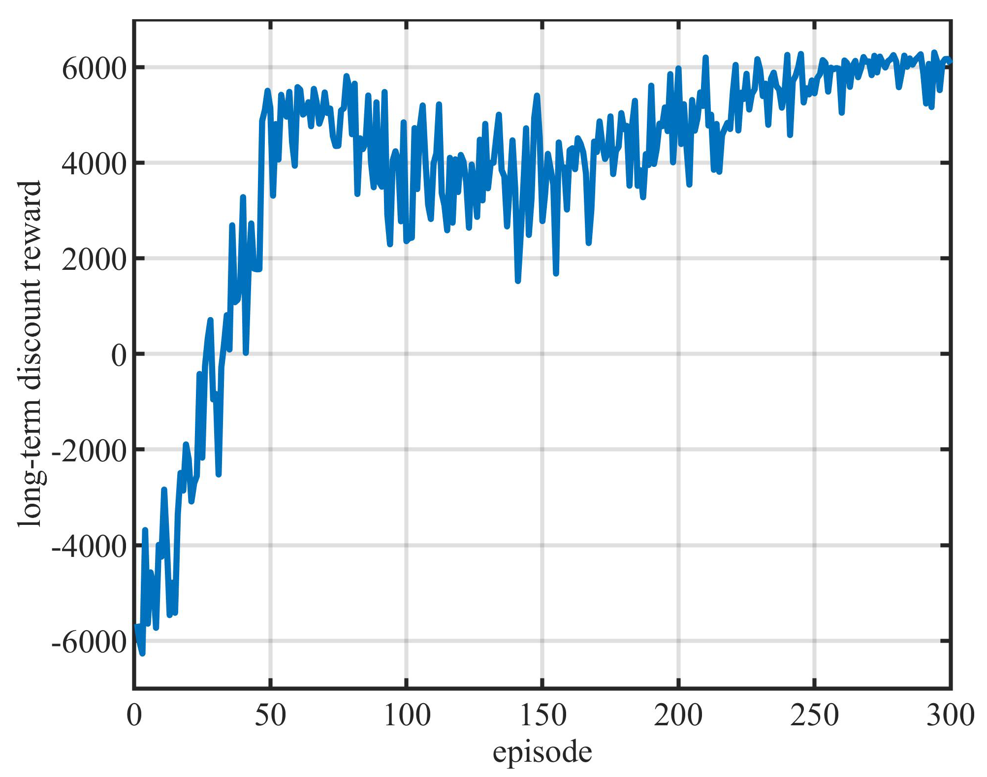
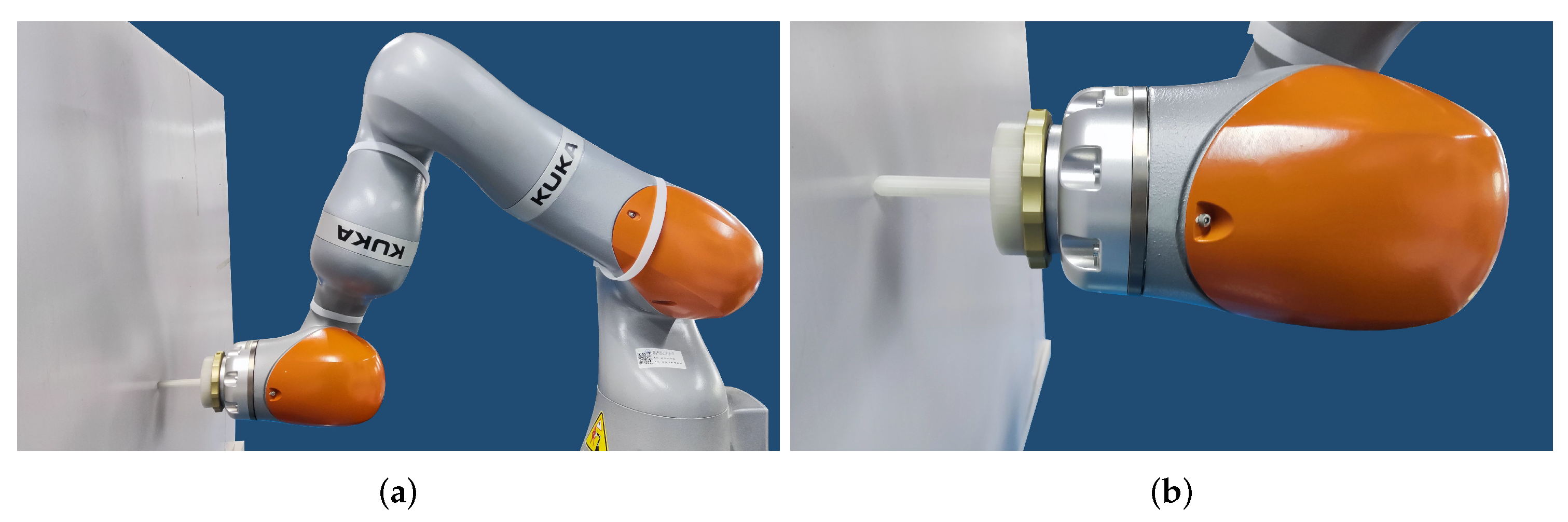
4.1. Moving along a Wall of Unknown Stiffness with a Constant Force

In this task shown in Figure 5, the two-link robot needs to move from a height of 0.2 m to a height of 0.6 m along the smooth vertical wall 0.6 m to its right while maintaining the horizontal contact force ${\mathbf{F}}_{\mathrm{contact}}$ of 50 N. The expected velocity in the horizontal direction is a bell-shaped curve, while the velocity in the vertical direction is constant. The wall’s stiffness $K_{\mathrm{wall}}=1000\mathrm{N}/\mathrm{m}$, damping $B_{\mathrm{wall}}=3\mathrm{N}·\mathrm{s}/\mathrm{m}$ and position is unknown to the robot.

With the fixed inertia parameter $M_{\mathrm{d}}=1\mathrm{kg}·{\mathrm{m}}^2$ and damping parameter $B_{\mathrm{d}}=100\mathrm{N}·\mathrm{s}/\mathrm{m}$ in the horizontal direction, the simulation results of the admittance control under different fixed stiffness parameters can be viewed in Figure 6. With the robot stiffness $K_{\mathrm{d}}=500\mathrm{N}/\mathrm{m}$, the contact force stabilizes at about $33\mathrm{N}$, which is smaller than the desired contact force. When the stiffness $K_{\mathrm{d}}$ is $2000\mathrm{N}/\mathrm{m}$, the contact force exceeds $75\mathrm{N}$, meaning that the contact force is positively related to the robot stiffness, and the stiffness parameter can be adjusted to make the contact force constant at $50\mathrm{N}$.

For this task, the contact force only exists in the horizontal direction, so the state consists of the position $x_1$, velocity ${\dot{x}}_1$ and contact force $F_1$ of the robot end-effector in this direction, while the action is the change of the stiffness. With ${\mathbf{s}}_t={\left[x_1,{\dot{x}}_1,F_1,1\right]}^{\mathrm{T}}$, the policy parameter $\psi ={\left[{\psi }_{x_1}^{\mathrm{T}},{\eta }_{x_1}\right]}^{\mathrm{T}}$ is a $5\times 1$ vector. The reward function is shown in Formula (18), and obtains the maximum value when $F_{\mathrm{contact}}=50\mathrm{N}$.

$$\begin{array}{c}\hfill r=\frac{1000}{100+{(F_{\mathrm{contact}}-50)}^2}.\end{array}$$

(18)

By training for 300 episodes with appropriate training parameters, the long-term discounted return curve shown in Figure 7 is obtained. With the increase of training episodes, the long-term discounted return value gradually rises and converges to the optimal.

Curves of how the contact force changes during training are drawn in Figure 8. At the beginning of the training, the contact force between the robot and the environment was less than $35\mathrm{N}$. With the increase of training episodes, the contact force gradually increased and reached the target contact force of $50\mathrm{N}$. At the $50\mathrm{th}$ episode, the contact force reached the target force at $2200\mathrm{ms}$ and exceeded it for the rest of the time. In the $150\mathrm{th}$ round, the contact force reached the target force earlier and stabilized above the target force. In the remaining training, the agent learned to control the rise and stability of the contact force. As for the $300\mathrm{th}$ round, the contact force reached the target force later, fell back and stabilized around the target force after exceeding it, giving the agent a higher long-term discount return.

The obtained optimal trajectories are applied to the real KUKA IIWA robot in Figure 9 where the end effector is perpendicular to the wall. The optimal trajectory in Cartesian space was firstly converted into the trajectory in joint space by the inverse kinematics model of the KUKA IIWA robot, and then executed by the mature joint position controller of the robot at a frequency of $175\mathrm{Hz}$.

In Figure 10, the end-effector trajectory of KUKA IIWA robot is similar to that of the two-link robot, and the maximum position deviation in the trajectory is less than $2\mathrm{mm}$, which ensures that the contact force only has a small deviation. Therefore, the method’s effectiveness of training the agent on a simple robot and applying the optimal trajectory to a complex robot to perform the same task is verified.

4.2. Opening a Door with Unknown Dynamics

For the door opening task shown in Figure 11, the horizontally placed two-link robot, which was the same as in the last task, needed to open the door in its upper right corner. The robot with the base coordinate at $[0\mathrm{m},0\mathrm{m}]$ needed to open a door with a length of $0.4\mathrm{m}$ that rotated around $[0.8\mathrm{m},0.8\mathrm{m}]$, and the end of the door was connected to the robot through a spherical joint.

In this task, the contact force came from the tangent and normal directions of the circle formed by the trajectory of the door’s end. In the tangential direction, the robot received the constraint force $F_{\tan }$ of the door’s dynamics, while in the normal direction, the robot’s stretching or squeezing on the door generated another force $F_{\tan }$. Both forces can be calculated by (19).

$$\begin{array}{cc}\hfill F_{\tan }& =M_{\mathrm{door}}{\ddot{\theta }}_{\mathrm{door}}+B_{\mathrm{door}}{\dot{\theta }}_{\mathrm{door}}+K_{\mathrm{door}\tan }({\theta }_{\mathrm{door}}-{\theta }_{\mathrm{door}\mathrm{init}})\hfill \\ \hfill F_{\mathrm{nom}}& =K_{\mathrm{door}\mathrm{nom}}(r-r_{\mathrm{origin}}).\hfill \end{array}$$

(19)

$M_{\mathrm{door}}=0.2667\mathrm{kg}·{\mathrm{m}}^2$ and $B_{\mathrm{door}}=30\mathrm{N}·\mathrm{s}/\mathrm{m}$ are the inertia and damping parameters, while $K_{\mathrm{door}\tan }=10,000\mathrm{N}/\mathrm{m}$ and $K_{\mathrm{door}\mathrm{nom}}=1\mathrm{N}/\mathrm{m}$ are the stiffness in different directions. ${\theta }_{\mathrm{door}}$ and its higher-order derivatives are the door angle, angular velocity, and angular acceleration, and ${\theta }_{\mathrm{door}\mathrm{init}}$ is the initial angle. $r_{\mathrm{origin}}$ and r are the door lengths before and after deformation, respectively.

The stiffness ellipse shown in Figure 12 was considered due to the contact force coming from multiple directions. For an ellipse with semi-major axis length a, semi-minor axis length b, ellipse’s magnitude $\pi ab$, shape $\frac{a}{b}$, and the orientation ${\theta }_{\mathrm{s}}$ between the major axis and the horizontal direction can completely summarize the stiffness ellipse. The stiffness in any direction $\theta$ is equal to the length L of the line segment $OA$ and can be calculated through (20) and (21).

$$\begin{array}{c}\hfill L{\mathbf{V}}_1{\mathbf{V}}_2\mathbf{E}{{\mathbf{V}}_2}^{\mathrm{T}}{{\mathbf{V}}_1}^{\mathrm{T}}L=1\end{array}$$

(20)

$$\begin{array}{cc}\hfill {\mathbf{V}}_1& =\left[\begin{array}{cc}\cos \left(\theta \right)& \sin \left(\theta \right)\end{array}\right]\hfill \\ \hfill {\mathbf{V}}_2& =\left[\begin{array}{cc}\cos \left({\theta }_{\mathrm{s}}\right)& \sin \left({\theta }_{\mathrm{s}}\right)\\ -\sin \left({\theta }_{\mathrm{s}}\right)& \cos \left({\theta }_{\mathrm{s}}\right)\end{array}\right]\hfill \\ \hfill \mathbf{E}& =\left[\begin{array}{cc}{}^1/{}_{a^2}& 0\\ 0& {}^1/{}_{b^2}.\end{array}\right]\hfill \end{array}$$

(21)

The desired trajectory contains an acceleration process and a deceleration process to ensure that the velocity and acceleration at the beginning and the end are both zero. Since the door’s geometric and dynamic information are agnostic to the robot, different circular input trajectories will result in different actual motions. When the input trajectory is a quarter-circle arc with a radius of 0.45 m and 0.35 m respectively, the motion trajectories of the end-effector are shown in Figure 13.

When the input expected trajectory radius is bigger than the door’s length, the robot tends to move outward along the door axis, and the door is pulled and deformed. The end-effector eventually moves along a trajectory outside the non-deformation trajectory of the door’s end, and the door opens more than ${90}^{\circ }$. Otherwise, the robot tends to squeeze the door inward. The door receives pressure while the robot moves along the inner trajectory and stays at less than ${90}^{\circ }$.

This task consists of two goals. (1) In order to protect the door’s safety, the normal contact force should be as small as possible; (2) At the end of the task, the door should be opened at a wide angle. The reward function adopted is shown in (22).

$$\begin{array}{c}\hfill r=\frac{1000}{100+{(F_{\mathrm{nom}}-0)}^2}+10(\pi /2-{\theta }_{\mathrm{door}}).\end{array}$$

(22)

Compared with the previous experiment, the robot position $x_1,x_2$, velocity ${\dot{x}}_1,{\dot{x}}_2$ and contact force $F_1,F_2$ in two directions were added to the state $\mathbf{s}={\left[x_1,{\dot{x}}_1,x_2,{\dot{x}}_2,F_1,F_2,1\right]}^{\mathrm{T}}$. The action vector was set to the amount of change in the size, shape, and main axis direction of the stiffness ellipse, that is, $\mathbf{a}={\left[{\mathbf{a}}_{\mathrm{magnitude}},{\mathbf{a}}_{\mathrm{shape}},{\mathbf{a}}_{\mathrm{orientation}}\right]}^{\mathrm{T}}$. For each action’s Gaussian distribution, there were seven parameters that affect the mean and one parameter that affects the standard deviation. Therefore, the corresponding policy parameters $\psi ={\left[{\psi }_{\mathrm{mag}}^{\mathrm{T}},{\psi }_{\mathrm{shape}}^{\mathrm{T}},{\psi }_{\mathrm{orient}}^{\mathrm{T}},{\eta }_{\mathrm{mag}},{\eta }_{\mathrm{shape}},{\eta }_{\mathrm{orient}}\right]}^{\mathrm{T}}\in {\mathbb{R}}^{24}$.

The long-term discount curve after training for 500 episodes is shown in Figure 14. The curve gradually accelerates and rises at first. After reaching a certain height, it turns and gradually converges.

The change of the contact force in the direction parallel to the door panel during the training process can be seen in Figure 15. After training, the maximum contact force during the door opening process gradually decreased from more than $17\mathrm{N}$ in the first episode to less than $8\mathrm{N}$ in the last, thus reducing the pressure of the robot on the door.

Figure 16 shows the trajectory of the end effector of the two-link robot and the corresponding stiffness ellipse at some point. We can see that the end effector gradually opens the door along the smooth arc curve, and the input trajectory is corrected to the actual trajectory by the admittance control, which is nearly coincident with the no-deformation trajectory. The stiffness ellipse is stretched horizontally and compressed vertically, and then rotates clockwise. It can be inferred that the optimal effect should be that the stiffness of the robot along the tangential direction of the door should be large enough so that the speed of the end effector in the tangential direction is close to the controller’s input. The force in the normal direction of the door will not improve the task performance and even damages the door’s structure, so the robot’s stiffness along the normal direction of the door should be small enough.

The optimal trajectory was used for the control of the KUKA IIWA robot, shown in Figure 17. It was first transferred to the joint space and performed by the robot’s own joint position controller, as in the last task. The end effector motion trajectory of the KUKA IIWA is shown in Figure 18. The robot could open the door to $64.4^{\circ }$ with a little deformation of the door, which is similar to the performance of the two-link robot. The feasibility of migrating the robot operation skills trained on the simple robot to the control of complex robots is verified.

5. Conclusions

In order to ensure the boundedness of action and differentiability of the policy simultaneously, artificial neurons were introduced into the eNAC algorithm to improve its robustness. To satisfy force control improvement in robot manipulators with different structures in an unstructured environment, the impedance control algorithm based on the modified eNAC algorithm was applied to adjust robots’ compliance online and was tested with two contact tasks. The wall-contacting and door-opening tasks results show that the modified eNAC algorithm presented in this paper can transfer the learned motion skills from the simulated robot to the real one. The complex robot can achieve a similar performance in the same experiment, and the difficulty of data collection and time consumption are reduced, which verifies the method’s effectiveness.

References

1. Prabakaran, V.; Elara, M.R.; Pathmakumar, T.; Nansai, S. Floor Cleaning Robot with Reconfigurable Mechanism. Autom. Constr. 2018, 91, 155–165. [Google Scholar] [CrossRef]
2. Bollini, M.; Tellex, S.; Thompson, T.; Roy, N.; Rus, D. Interpreting and Executing Recipes with a Cooking Robot. In Experimental Robotics; Desai, J.P., Dudek, G., Khatib, O., Kumar, V., Eds.; Springer International Publishing: Berlin/Heidelberg, Germany, 2013; Volume 88, pp. 481–495. [Google Scholar] [CrossRef] [Green Version]
3. Wang, Z.; Majewicz Fey, A. Deep Learning with Convolutional Neural Network for Objective Skill Evaluation in Robot-Assisted Surgery. Int. J. CARS 2018, 13, 1959–1970. [Google Scholar] [CrossRef] [PubMed] [Green Version]
4. Siciliano, B.; Sciavicco, L.; Villani, L.; Oriolo, G. Robotics Modelling, Planning and Control; Advanced Textbooks in Control and Signal Processing; Springer: London, UK, 2009. [Google Scholar] [CrossRef]
5. Dini, P.; Saponara, S. Model-Based Design of an Improved Electric Drive Controller for High-Precision Applications Based on Feedback Linearization Technique. Electronics 2021, 10, 2954. [Google Scholar] [CrossRef]
6. Bernardeschi, C.; Dini, P.; Domenici, A.; Saponara, S. Co-Simulation and Verification of a Non-linear Control System for Cogging Torque Reduction in Brushless Motors. Int. Conf. Softw. Eng. Form. Methods 2020, 12226, 3–19. [Google Scholar] [CrossRef]
7. Sheng, X.; Zhang, X. Fuzzy Adaptive Hybrid Impedance Control for Mirror Milling System. Mechatronics 2018, 53, 20–27. [Google Scholar] [CrossRef]
8. Fu, Y.; Lin, W.; Yu, X.; Rodriguez-Andina, J.J.; Gao, H. Robot-Assisted Teleoperation Ultrasound System Based on Fusion of Augmented Reality and Predictive Force. IEEE Trans. Ind. Electron. 2022, 1–8. [Google Scholar] [CrossRef]
9. Cao, H.; Chen, X.; He, Y.; Zhao, X. Dynamic Adaptive Hybrid Impedance Control for Dynamic Contact Force Tracking in Uncertain Environments. IEEE Access 2019, 7, 83162–83174. [Google Scholar] [CrossRef]
10. Lin, W.; Liu, C.; Guo, H.; Gao, H. Hybrid Visual-Ranging Servoing for Positioning Based on Image and Measurement Features. IEEE Trans. Cybern. 2022, 1–10. [Google Scholar] [CrossRef]
11. Stolt, A.; Linderoth, M.; Robertsson, A.; Johansson, R. Force Controlled Robotic Assembly without a Force Sensor. In Proceedings of the 2012 IEEE International Conference on Robotics and Automation, St Paul, MN, USA, 14–18 May 2012; IEEE: Piscataway, NJ, USA, 2012; pp. 1538–1543. [Google Scholar] [CrossRef] [Green Version]
12. Nouri, M.; Fussell, B.K.; Ziniti, B.L.; Linder, E. Real-Time Tool Wear Monitoring in Milling Using a Cutting Condition Independent Method. Int. J. Mach. Tools Manuf. 2015, 89, 1–13. [Google Scholar] [CrossRef]
13. Peters, J.; Schaal, S. Policy Gradient Methods for Robotics. In Proceedings of the 2006 IEEE/RSJ International Conference on Intelligent Robots and Systems, Beijing, China, 9–13 October 2006; IEEE: Piscataway, NJ, USA, 2006; pp. 2219–2225. [Google Scholar] [CrossRef] [Green Version]
14. Dayanidhi, S.; Hedberg, A.; Valero-Cuevas, F.J.; Forssberg, H. Developmental Improvements in Dynamic Control of Fingertip Forces Last throughout Childhood and into Adolescence. J. Neurophysiol. 2013, 110, 1583–1592. [Google Scholar] [CrossRef] [Green Version]
15. Campeau-Lecours, A.; Otis, M.J.D.; Gosselin, C. Modeling of Physical Human–Robot Interaction: Admittance Controllers Applied to Intelligent Assist Devices with Large Payload. Int. J. Adv. Robot. Syst. 2016, 13, 172988141665816. [Google Scholar] [CrossRef] [Green Version]
16. Sutton, R.S.; Barto, A.G. Reinforcement Learning: An Introduction, 2nd ed.; Adaptive Computation and Machine Learning Series; The MIT Press: Cambridge, MA, USA, 2018. [Google Scholar]
17. Jung, S.; Hsia, T.; Bonitz, R. Force Tracking Impedance Control of Robot Manipulators Under Unknown Environment. IEEE Trans. Contr. Syst. Technol. 2004, 12, 474–483. [Google Scholar] [CrossRef]
18. Peters, J.; Vijayakumar, S.; Schaal, S. Reinforcement Learning for Humanoid Robotics. In Proceedings of the Third IEEE-RAS International Conference on Humanoid Robots, Karlsruhe-Munich, Germany, 29–30 September 2003; pp. 1–20. [Google Scholar]
19. Kim, B.; Park, J.; Park, S.; Kang, S. Impedance Learning for Robotic Contact Tasks Using Natural Actor-Critic Algorithm. IEEE Trans. Syst. Man Cybern. B 2010, 40, 433–443. [Google Scholar] [CrossRef]
20. Beltran-Hernandez, C.C.; Petit, D.; Ramirez-Alpizar, I.G.; Nishi, T.; Kikuchi, S.; Matsubara, T.; Harada, K. Learning Force Control for Contact-rich Manipulation Tasks with Rigid Position-controlled Robots. IEEE Robot. Autom. Lett. 2020, 5, 5709–5716. [Google Scholar] [CrossRef]
21. Haarnoja, T.; Zhou, A.; Abbeel, P.; Levine, S. Soft Actor-Critic: Off-Policy Maximum Entropy Deep Reinforcement Learning with a Stochastic Actor. arXiv 2018, arXiv:1801.01290. Available online: http://xxx.lanl.gov/abs/1801.01290 (accessed on 5 March 2022).
22. Siciliano, B.; Khatib, O. (Eds.) Springer Handbook of Robotics; Springer International Publishing: Cham, Switzerland, 2016. [Google Scholar] [CrossRef]
23. Lee, K.; Buss, M. Force Tracking Impedance Control with Variable Target Stiffness. IFAC Proc. Vol. 2008, 41, 6751–6756. [Google Scholar] [CrossRef]
24. Sutton, R.S.; McAllester, D.; Singh, S.; Mansour, Y. Policy Gradient Methods for Reinforcement Learning with Function Approximation. Adv. Neural Inf. Process. Syst. 1999, 7, 1057–1063. [Google Scholar]
25. Park, J.; Kim, J.; Kang, D. An RLS-Based Natural Actor-Critic Algorithm for Locomotion of a Two-Linked Robot Arm. In Computational Intelligence and Security; Springer: Berlin/Heidelberg, Germany, 2005; Volume 3801, pp. 65–72. [Google Scholar] [CrossRef] [Green Version]
26. Stulp, F.; Buchli, J.; Ellmer, A.; Mistry, M.; Theodorou, E.A.; Schaal, S. Model-Free Reinforcement Learning of Impedance Control in Stochastic Environments. IEEE Trans. Auton. Ment. Dev. 2012, 4, 330–341. [Google Scholar] [CrossRef] [Green Version]
27. Dini, P.; Saponara, S. Design of Adaptive Controller Exploiting Learning Concepts Applied to a BLDC-Based Drive System. Energies 2020, 13, 2512. [Google Scholar] [CrossRef]
28. Dini, P.; Saponara, S. Processor-in-the-Loop Validation of a Gradient Descent-Based Model Predictive Control for Assisted Driving and Obstacles Avoidance Applications. IEEE Access 2022, 10, 67958–67975. [Google Scholar] [CrossRef]
29. Safeea, M.; Neto, P. KUKA Sunrise Toolbox: Interfacing Collaborative Robots with MATLAB. IEEE Robot. Autom. Mag. 2019, 26, 91–96. [Google Scholar] [CrossRef] [Green Version]
30. Corke, P. Robotics, Vision and Control; Springer Tracts in Advanced Robotics; Springer International Publishing: Cham, Switzerland, 2017; Volume 118. [Google Scholar] [CrossRef]
Figure 1. The control loops for impedance control (the upper one) and admittance control (the lower one). x d , F d are the desired trajectory and desired contact force; x c , F c are the inputs of the robot controllers; x , F ext are the actual motion trajectory of the robot and contact force, respectively. The dimensions and composition of the above vectors are related to specific experiments.
Electronics 12 00411 g001
Figure 2. The realization of the admittance control. The definitions of symbols are the same as those in Figure 1.
Electronics 12 00411 g002
Figure 3. The main components in Actor-Critic and its execution flow.
Electronics 12 00411 g003
Figure 4. The simulated robot was selected as a two-link robot. The joint angles are, respectively, q 1 and q 2 .
Electronics 12 00411 g004
Figure 5. The scene of the wall-contacting task. The two-link robot with two revolute joints needs to keep a constant contact force while moving along a wall with unknown stiffness. x 1 is the direction toward the inside of the wall, and x 2 is the direction upward along the wall.
Electronics 12 00411 g005
Figure 6. Robot’s contact forces with the wall in the horizontal direction under different stiffness parameters.
Electronics 12 00411 g006
Figure 7. The curve of the long-term discount return with respect to the training episode in the wall-contacting task.
Electronics 12 00411 g007
Figure 8. The contact force curves between the robot and the wall of different episodes.
Electronics 12 00411 g008
Figure 9. Different perspectives of the IIWA KUKA. The end effector needs to move up a certain distance while remaining perpendicular to the wall. (a) The overall perspective. (b) The local perspective.
Electronics 12 00411 g009
Figure 10. Trajectory of end-effector of two-link robot and KUKA IIWA robot.
Electronics 12 00411 g010
Figure 11. The scene of the door-opening task. The two-link robot with two revolute joints needs to opening a door with unknown length and dynamics.
Electronics 12 00411 g011
Figure 12. The two-link robot and its stiffness eclipse under the admittance control.
Electronics 12 00411 g012
Figure 13. The end-effector’s actual motions with different desired x d in the door-opening task. The actual trajectory of the end effector differs significantly from the desired trajectory due to door’s constraints. (a) Simulation results in a quarter-circle arc with a radius of 0.35 m as desired trajectory x d . (b) Simulation results in a quarter-circle arc with a radius of 0.45 m as x d .
Electronics 12 00411 g013aElectronics 12 00411 g013b
Figure 14. The curve of the long-term discount return with respect to the training episode in the door-opening task.
Electronics 12 00411 g014
Figure 15. The curve of the contact force between the robot and the door in the direction parallel to the panel in different training episodes.
Electronics 12 00411 g015
Figure 16. The desired trajectory, the trajectory of the end of the undeformed door, the trajectory of the end effector of the two-link robot and the corresponding stiffness ellipse of some trajectory points in the door-opening task.
Electronics 12 00411 g016
Figure 17. Different perspectives of the KUKA IIWA. The robot needs to open the door while the end effector remains parallel to the door. (a) Perspective from the side. (b) Perspective from the above.
Electronics 12 00411 g017
Figure 18. The desired trajectory, the trajectory of the end of the undeformed door, the trajectory of the KUKA IIWA robot’s end effector for the door-opening task.
Electronics 12 00411 g018
Disclaimer/Publisher’s Note: The statements, opinions and data contained in all publications are solely those of the individual author(s) and contributor(s) and not of MDPI and/or the editor(s). MDPI and/or the editor(s) disclaim responsibility for any injury to people or property resulting from any ideas, methods, instructions or products referred to in the content.