Smart Electricity Meter Load Prediction in Dubai Using MLR, ANN, RF, and ARIMA

Abstract

Load forecasting is one of the main concerns for power utility companies. It plays a significant role in planning decisions, scheduling, operations, pricing, customer satisfaction, and system security. This helps smart utility companies deliver services more efficiently and analyze their operations in a way that can help optimize performance. In this paper, we propose a study of different techniques: multiple linear regression (MLR), random forests (RF), artificial neural networks (ANNs), and automatic regression integrated moving average (ARIMA). This study used electricity consumption data from Dubai. The main objective was to determine the load demand for the next month in the whole country and different municipal areas in Dubai, as well as to assist a utility company in future system scaling by adding new power stations for high-demand regions. The results showed that the accuracy of using ARIMA was about 93% when working with only a single district, but both ANN and RF achieved excellent accuracy of about 97% in all cases. In addition, the mean absolute percentage errors improved from 2.77 and 2.17 to 0.31 and 0.157 for ANN and RF, respectively, after anomaly elimination and the use of our proposal. Therefore, the use of an ANN for such data types is recommended in most cases, particularly when working on a complete dataset. Additionally, both the ANN and RF models are good choices when working on a single-category region because they both attained the same accuracy of almost 91.02 percent.

1. Introduction

The smart grid (SG) is the future of the electrical industry, as it uses upgraded power system components to replace the old electrical infrastructure. It provides two-way digital communication between the electricity plant and the consumer. Furthermore, it assists in cost and energy savings and ensures that the energy supply chain is transparent and reliable. The increased complexity of smart grids has resulted in significant efforts to control distribution levels, develop fault detection techniques, and ensure system reliability [1].

Smart meters (SMs) are the most important components of a smart grid. They record the energy usage and send data to utility suppliers. In addition, they provide dependable real-time monitoring, automatic data gathering, user interaction, and power control. Enormous amounts of data are generated from SMs [2]. The data from smart meters are raw data that require data analysis techniques to recognize, transform, and obtain conclusions [3].

For several reasons, smart utility companies in the electric, gas, and water sectors face challenges in expanding their use of smart meters. The main reasons are the need for a low-cost network to carry all meters’ communications, the complexity of collecting and analyzing data from a large number of meters, and the ease of smart meter management and expansion [4,5].

New applications that use smart grids provide various benefits to customers. They will be able to monitor usage for a given period by using the data received from these measurements. This will aid in the development of solutions for optimizing the use of power and water resources [6].

The accurate processing of data collected by smart meters is a major research topic. This helps utility companies with the following [7,8,9,10,11,12]:

• Load forecasting, which plays a significant role in planning decisions, scheduling, operation, pricing, customer satisfaction, and system security [13].
• Developing new pricing plans to encourage consumers to reduce peak demand and better manage energy consumption.
• Offering different pricing schemes where consumers are charged higher prices during peak hours.
• Providing essential insights into electricity usage behaviors during working days and holidays.
• Detecting malfunctioning meters and targeting them for replacement.
• The detection of abnormal consumption patterns that indicate an electricity theft.

1.1. The Literature and Related Work

Several techniques have been proposed for smart-meter data analysis and load forecasting, including time-series analysis, regression analysis, artificial neural networks (ANNs), support vector machines (SVMs), fuzzy logic (FL), and genetic algorithms (GAs). In addition, hybrid techniques combine two or more techniques to overcome the limitations of single techniques.

Load forecasting can be categorized into four classes in terms of the forecast depth [14].

Very-short-term load forecasting (VSTLF) [15] is popular for load forecasting from a few seconds to a few minutes. Short-term load forecasting (STLF) is used for lead times ranging from a few minutes to a few hours. This is the primary source of information for all daily and weekly activities, including generation commitment and scheduling, and it is crucial for system operations. By including econometric variables and expanding the model to a longer horizon, STLF can be converted into MTLF and LTLF.

Medium-term load forecasting (MTLF) [16] is generally used to forecast loads for a few days to a few months. Finally, long-term load forecasting (LTLF) [17] is used for a period of a few months to several years, which is helpful for generation growth planning.

The authors of [18] proposed a short-term load forecasting framework based on big data technologies. It used a decision tree to classify the daily load patterns of individual loads. A suitable load forecasting model was then selected for each load pattern. The total load was obtained by aggregating the forecasting results of the individual loads.

The authors of [19] created and implemented an embedded distribution panelboard system. The connected end-node sensors gathered the voltage and current information to calculate the power and energy usage. An IoT platform received the computed data and measurements that were gathered and offered cloud-computing capabilities for data analysis and action facilitation.

In [20], a hybrid forecast model for short-term electricity load and price prediction was proposed, and it used wavelet transform and feature selection techniques to handle fluctuations in the electricity load. Although the performance of the model was successfully validated based on load and price data collected from the Pennsylvania–New Jersey–Maryland (PJM) electricity market, it was not suitable for individual household prediction because it aggregated load forecasting for a single region.

A CNN sequence-to-sequence model with an attention mechanism and multitask learning was used in [21]. It extracted useful features from the input data by using a CNN. Then, the weight matrix was updated to improve the forecasting accuracy.

In [22], several deep learning methods were compared to forecast the electric power consumption in buildings. Long short-term memory (LSTM)/GRU with multiple layers was used; the sequence-to-sequence model consisted of two recurrent neural networks and a sequence-to-sequence model with attention mechanisms.

Jeyaranjani and Devaraj proposed a deep neural network (DNN) for residential load forecasting. The network architecture was implemented with five hidden layers [23].

In [24], a deep learning (DL) prediction model was suggested to precisely forecast hourly load consumption. Then, the predicted data for a real-time decision were used to decide the actions needed to reduce the peak load demand.

W. Chandramitasari et al. [25] suggested a technique that combined LSTM and a feed-forward neural network. They predicted the amount of electricity used every 30 min for the next day. This study focused only on consumption in a manufacturing company and did not consider other types of consumption, such as residential, commercial, or government consumption.

Moreover, many articles have proposed hyperparameter tuning techniques that are combinations of statistical models and ML models or combinations of various ML models to provide a more accurate forecast than using only one machine learning technique [14].

In [26], a hyperparameter tuning technique called sequential grid search was based on the widely used grid search for ANN and hybrid models. It was used to forecast the daily electricity consumption in Thailand. It combined the advantages of different models to solve the overfitting problem and improper kernel function selection when dealing with nonlinear data.

In addition, in [27], a hybrid model of the wavelet transform, simulated annealing, and feed-forward ANN was proposed to predict electricity consumption in Beijing, China, one day ahead. The developed approach was able to predict the demand for electricity in a microgrid with a tolerably small error and a reasonable amount of computing time.

In [28], the authors used two years of residential customer data in Bangladesh to train and test different types of machine learning (ML) regression algorithms to predict the power consumption for the following day. The results showed that SVR was associated with better outcomes. The limitations of this work were that it focused only on residential customers and neglected utility load prediction.

In [29], deep learning algorithms and decision trees with drift detection techniques were discussed to forecast the electricity consumption of two buildings on the Valladolid University campus. Three techniques were used: two active and one passive. The passive approach involved retraining the models every 24 h under the assumption that they should be frequently updated. However, the active techniques were based on a variable-length window approach.

Admir Jahić et al. [30] proposed an ANN-based model to determine missing power measurement readings to distinguish between truly disconnected loads and loads with no consumption. Missing power measurement readings were replaced with pseudo-measurements. Despite its simplicity, this approach required ANN retraining due to weekends, holidays, and seasonal variations.

Other solutions focused on detecting malfunctioning smart meters and abnormal consumption patterns that indicate electricity theft have been proposed. The authors of [31] focused on detecting inaccurate smart meters. The model was based on long short-term memory (LSTM) and a modified CNN. It collected the difference between the predicted and observed values, and the meters that could not accurately measure electricity were located.

In [32], a big data modeling method was designed to identify abnormal data detection through the spectral distribution of the random matrix theory.

The solution suggested in [33] used a support vector machine to detect fraud by utilizing the predictability of the client consumption profile. The authors of [34] proposed an approach that used a decision tree to identify abnormal data and categorize them with different degrees of energy loss. The data were then clustered to obtain different energy consumption behaviors. The meter error was calculated from the solution of the matrix equation after constructing the data matrix.

Table 1. A comparison between the related work and the proposed work.

Paper	Contribution	Achievements	Limitations
[12]	Hourly average load prediction of a residential house.	A comparison of load forecasting models using an ANN and ELM.	Focused only on consumption by residential customers.
[19]	Proposed a long short-term memory (LSTM)-based forecasting algorithm.	Good capabilities of forecasting based on load and price data collected from the PJM electricity market.	Not suitable for individual household prediction, as it aggregated load forecasting for a single region.
[20]	Proposed a distribution panelboard system.	A low-voltage electrical distribution panelboard with real-time load monitoring and the capability of domestic load forecasting.	The process did not consider the consumer level or features such as fault detection and identification.
[25]	A proposed approach for load forecasting for the next day every 30 min.	Performed forecasting with additional information to minimize the loss of forecasting for the next day every 30 min.	Focused only on consumption in a manufacturing company.
[28]	Forecasting of the power consumption for the next day	A circuit design of GSM-based smart energy with a microcontroller was used in calculating the current, voltage, energy, and cost. The GSM module informed the customers about their daily power consumption	The work was focused on the customer side and neglected the prediction of the utilities’ load. In addition, it focused only on residential customers.
[30]	Detection of missing power meter readings.	Determined missing power measurement readings to distinguish between them and true loads with no consumption.	Required ANN retraining due to weekends, holidays, and seasonal variations.
Our work	Forecasting of the monthly load consumption for a region in the Middle East.	Determined the demand for the next month in different municipal areas in Dubai. Selection of the proper algorithm that was suitable for the DEWA data. Detection of anomaly values in the data. Mimicking of the influence of the weather on the model.	Hourly or daily consumption analysis was not included in this study due to the lack of this information in this dataset.

presents a comparison between related works and our proposed work.

1.2. Motivation and Contribution

The motivation behind this study was the enhancement of electricity consumption predictions in Middle Eastern countries. Electricity consumption data are collected hourly or daily in most parts of the world. The issue in the Middle East is that, in most countries, electric meter readings are still collected monthly, which makes predictions and correlations poor. Additionally, there is a lack of research focusing on the consumption behavior of this region.

Overcoming the problems of poor correlation and the low amount of data per customer requires powerful forecasting techniques and forecasting customization.

Forecasting the electricity consumption of countries is an important research area, and many methods have been applied to this problem.

The contributions of this study can be summarized as follows:

• Forecasting of electricity consumption is used to determine the demand for the next month in different municipal areas in Dubai.
• By adding new power stations to high-demand regions, utility industry decision makers can anticipate future power consumption with the lowest possible error rate and future scaling of the grid.
• Three different machine learning techniques (MLR, RF, and ANN) are used, and their performance in terms of the mean absolute error (MAE), root mean squared error (RMSE), mean absolute percentage error (MAPE), and correlation coefficient ($R^2$) is compared.
• The prediction accuracy is enhanced by adding a new variable to the dataset to mimic the influence of the weather on the model.
• The prediction accuracy is enhanced by detecting anomaly values by using a one-class SVM.
• Principal component analysis (PCA) is used as a feature selection technique that determines the weight of each predictor.
• An ARIMA time-series model is used to predict consumption for the whole of Dubai, one district, and one customer.
• The study focused on data from Dubai, as we preferred working with new and real traces of smart meters. This was due to the lack of research that focused on the consumption behavior of this region (Middle Eastern countries), which has resulted in poor electricity load forecasting.
• The proper algorithm that is suitable for DEWA data is selected.

1.3. Paper Organization

The remainder of this paper is organized as follows. Section 2 describes the method and the dataset. Section 3 presents the results and discussion. Finally, Section 4 presents the conclusion and directions for future work.

2. Materials and Methods

The details of the techniques employed, the dataset, and the data pretreatment methodology are described in this section. Figure 1 shows a summary of the methodology used in the proposed method.

The first stage was data preprocessing, which included data cleaning, duplicate removal, fixing spelling and syntax errors, handling missing values, identifying and eliminating outliers, feature selection, and sampling.

The second stage included the use of MLR, RF, and ANN algorithms for load prediction while working on the original dataset.

The third stage included our method of enhancing prediction accuracy by detecting anomaly values by using a one-class SVM and adding a new feather to mimic the influence of the weather.

2.1. Forecasting Algorithms

Machine learning is the process of extracting information from data. It is also known as predictive analytics or statistical learning and is a subject of study at the crossroads of statistics, artificial intelligence, and computer science. Over the last several years, machine learning techniques have become increasingly prevalent in daily life. The most effective machine learning algorithms are those that automate decision-making processes by generalizing them from existing examples. This approach is known as supervised learning (SL). Using supervised learning, a machine is trained by using a set of labeled data, where each element is composed of given input/outcome pairs [35]. The machine learns the relationship between the input and outcome, and the goal is to predict behavior or make a decision based on previously provided data. This can assist in building a model for predicting outcomes in future cases. Deciding among them is important because multiple techniques are employed to achieve the same goal. The required output determines the algorithm to be used. No single optimal algorithm continuously produces the best results. Moreover, it is crucial to test several algorithms to understand how they function. There are several methods for improving performance. The relative performance of two methods may be altered after analyzing the input data; however, the most important aspect is that developing the optimal algorithm is an iterative trial-and-error process [36,37,38].

2.1.1. Multiple Linear Regression (MLR)

MLR is a regression model that involves more than one regressor variable. The relationship between two or more independent variables and one dependent variable is estimated by using this method. The dependent and independent variables have a linear relationship. The correlation between unrelated variables is not very high [39,40].

$$Y_i={\beta }_0+{\beta }_1{x}_{i1}+{\beta }_2{x}_{i2}+\dots +{\beta }_p{x}_{ip}+ϵ$$

(1)

where i = 1, 2, 3, …, n.

$Y_i$ is the dependent variable, $x_i$ is the independent variable, ${\beta }_0$ is the value of Y when all independent variables ($x_1$ through $x_p$) are equal to zero (constant term), ${\beta }_p$ are the estimated regression coefficients (there are p + 1 (${\beta }_0$, ${\beta }_1$, ${\beta }_2$ …${\beta }_p$)), and $ϵ$ is the model’s error term (also known as the residuals).

In matrix representation, this is

$$Y=X\beta +ϵ$$

(2)

$$C{U}_{n\times 1}=\left[\begin{array}{c}C{U}_1\\ C{U}_2\\ ⋮\\ C{U}_n\end{array}\right],x_{n\times 4}=\left[\begin{array}{cccc}1& C_{12}& R{G}_{13}& C{P}_{14}\\ 1& C_{22}& R{G}_{23}& R{G}_{24}\\ ⋮& ⋮& ⋮& ⋮\\ 1& C_{n2}& R{G}_{n3}& C{P}_{n4}\end{array}\right],{\beta }_{4\times 1}=\left[\begin{array}{c}{\beta }_0\\ {\beta }_1\\ {\beta }_2\\ {\beta }_3\end{array}\right],{ϵ}_{n\times 1}=\left[\begin{array}{c}{ϵ}_1\\ {ϵ}_2\\ ⋮\\ {ϵ}_n\end{array}\right]$$

where $RG$ is the rate category, $CP$ is the consumption period, C is the community, and $CU$ is the consumption unit.

2.1.2. Random Forest (RF)

Random forest is a machine learning algorithm that is a supervised learning technique. It can be used for classification and regression prediction [41]. It is based on the idea of ensemble learning, which is a technique for integrating many classifiers to solve complex problems and enhance the performance of a model [42]. Ensembles build many solutions for a given issue and, in order to create the final result, incorporate all of the single results to form the best solution [43].

It achieves better performance than that obtained from the constituent learning algorithms alone. It constructs N trees by using a decision tree algorithm. A larger number of trees leads to higher accuracy and overcomes the overfitting problem.

They are trained by using the “bagging” method. This is a method within ensemble algorithms that ensures that different trees are trained on different subsets of the dataset to ensure that all trees are not correlated with each other. Each decision tree makes a prediction. It takes the prediction from each tree and then predicts the final output based on the majority votes of predictions. The weaknesses of the decision tree algorithm were eliminated by this algorithm [44].

It constructs N trees based on a decision tree algorithm, as shown in Figure 2. The decision tree breaks a dataset down into smaller subsets based on the standard deviation. A decision leaf is split into two or more branches, which represent the value of the attribute under examination. The splits are performed with thresholds that provide the minimum sum of squared residuals.

The residual sum of squares (RSS) with the minimum threshold is a candidate for the tree root. When the algorithm can no longer add further information to the leaf, the node stops splitting and becomes a leaf node.

$${ϵ}_i=y_i-{\widehat{y}}_i$$

(3)

$$RSS=\sum _{i=1}^n{(y_i-{\widehat{y}}_i)}^2$$

(4)

$$RSS={ϵ}_1^2+{ϵ}_2^2+\cdots +{ϵ}_n^2$$

(5)

where $ϵ$ is the model’s error term and $RSS$ is the residual sum of squares.

The parameters to be adjusted when running the model are:

• “$N\_estimators$” is the number of trees to build in the forest.
• “$Max\_depth$” is the maximum depth of a tree.
• “$Minimum\_leaf\_samples$” is the minimum number of samples required to be at a leaf node.
• “$Max\_features$” is the number of features to use for splitting.

The number of features for achieving the best split can equal the number of input features, sqrt(n_features), or ${log}_2$ (n_features).

2.1.3. Artificial Neural Network (ANN)

Artificial neural networks are a subfield of artificial intelligence (AI). They are designed to mimic the human brain by analyzing and processing information similarly to humans. This allows computer programs to identify patterns and resolve common problems in the fields of deep learning, machine learning, and AI.

In the human brain, neurons are linked to one another. Similarly to natural neural networks, artificial neural networks feature interconnected neurons, which can have any number based on the needs of the application. Neurons are connected to each other in several layers of the network.

Neurons communicate with one another through electric pulses. Each neuron has a threshold and associated weight. Any node whose output is greater than the specified threshold value is activated and begins sending data to the next layer of the network [45], and the importance of the node is determined by associating weights.

The most common structure of an artificial neural network comprises an input layer, one or more hidden layers, and an output layer. The input layer receives data, which are often vectors. The number of parameters in the input vector is typically equal to the number of input nodes in the input layer. It preprocesses the data and passes them to the hidden layers. The main processing happens in the hidden layer. There may be one or more hidden layers.

The hidden layers use an activation function as a processing function. There are many different activation functions: linear, binary sigmoid, and bipolar sigmoid functions. A linear activation function multiplies the input by weights and creates an output. A binary sigmoid function provides an output between zero and one. A bipolar sigmoid gives the output between the negative and positive ones. The output layer can be connected to both the input and hidden layers. Sometimes, the information is sent back to the input layer from the output layer. This yields the final prediction value [46,47].

$$C{U}_i=C_i.{\omega }_1+R{G}_i.{\omega }_2+C{P}_i.{\omega }_3$$

(6)

The numbers of layers and nodes in each hidden layer are the two primary hyperparameters for artificial neural networks, and they affect the design or topology of the network. Additionally, the size of the input layer depends on the number of input features. The prediction was performed by using a typical neural network with one hidden layer. The number of hidden neurons was selected by using a trial-and-error method. Figure 3 shows a sample ANN with seven neurons.

2.1.4. Automatic Regression Integrated Moving Average (ARIMA)

ARIMA is a mathematical model used in time-series analysis. It is a powerful tool for predicting the future values of a series based on past values. ARIMA models are based on the assumption that a series is stationary, meaning that the mean and variance of the series remain constant over time.

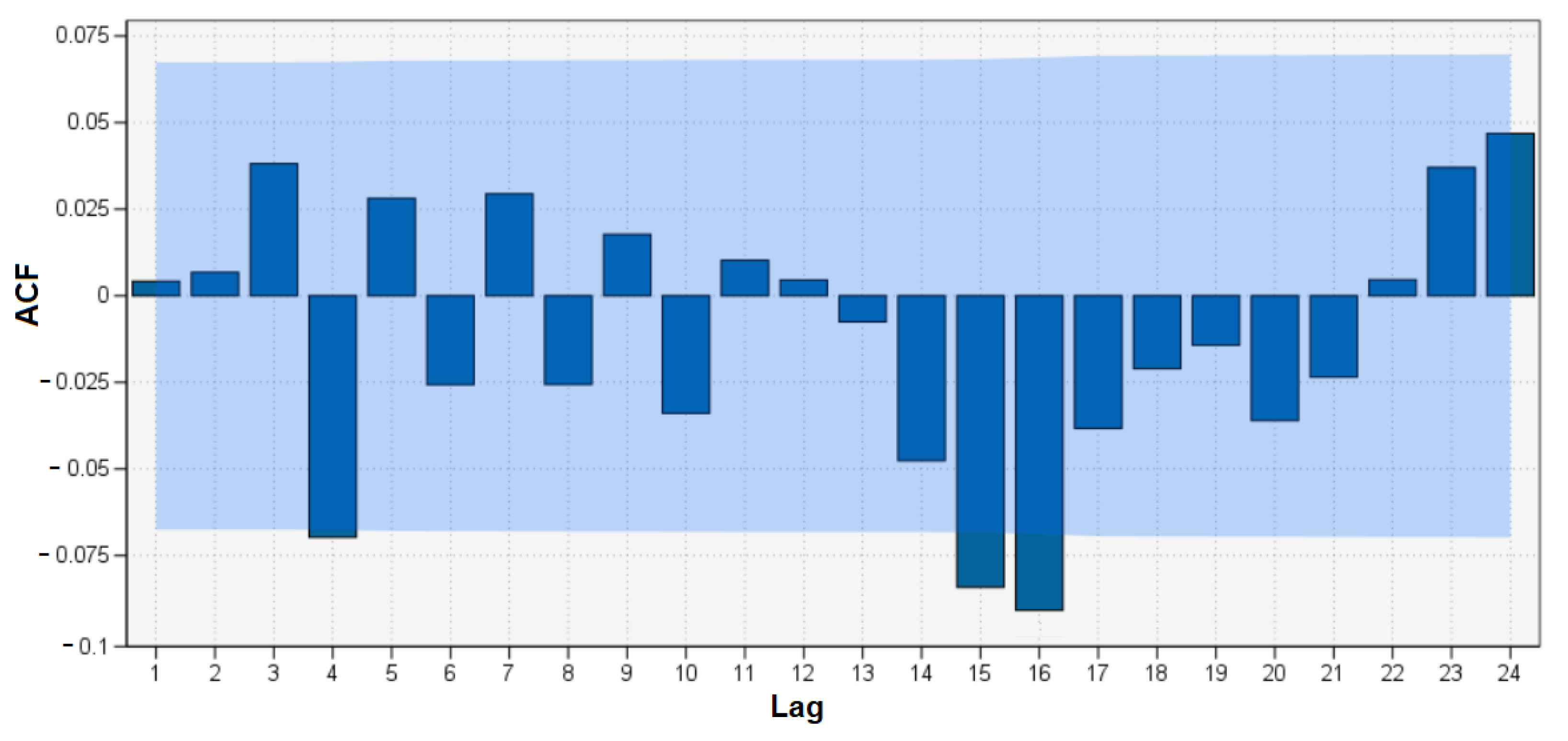
The components of the ARIMA(p,d,q) model are the autoregressive (AR) component, the integrated (I) component, and the moving average (MA) component. The AR component uses past values of the series to predict future values. The order of the AR component is represented by (p). The optimal value of (p) is determined with a partial autocorrelation function (PACF) plot, as shown in Figure 4. The I component is used to remove any non-stationary components from the series. (d) represents the total differencing steps performed by the I component to make the time series stationary. The MA component uses past errors to predict future values. The order of the MA component is represented by (q). By using an autocorrelation function (ACF) plot, we determined the optimal value for (q), as shown in Figure 5.

The equation for the AR model is:

$$C{U}_t={\beta }_1+{\varphi }_{1}C{U}_{t-1}+{\varphi }_{2}C{U}_{t-2}+\dots +{\varphi }_{p}C{U}_{t-p}$$

(7)

where $\varphi$ is the respective weight of the corresponding lagged observation.

The equation for the MA model is:

$$C{U}_t={\beta }_2+{\omega }_1{ϵ}_{t-1}+{\omega }_2{ϵ}_{t-2}+\dots +{\omega }_q{ϵ}_{t-q}+{ϵ}_t$$

(8)

where $ϵ$ represents the errors observed at respective lags and $\omega$ represents the respective weights of the corresponding error depending on the correlations.

When we combine the AR and MA equations, we get:

$$C{U}_t=({\beta }_1+{\beta }_2)+({\varphi }_{1}C{U}_{t-1}+\dots +{\varphi }_{p}C{U}_{t-p})+({\omega }_1{ϵ}_{t-1}+\dots +{\omega }_q{ϵ}_{t-q}+{ϵ}_t)$$

(9)

If the mean is non-constant, we need to calculate the difference between consecutive observations.

$$\mathrm{for}\mathrm{d}=1,Z_t=C{U}_{t+1}-C{U}_t$$

(10)

$$\mathrm{for}\mathrm{d}=2,Q_t=Z_{t+1}-Z_t$$

(11)

2.2. Dataset

The dataset was provided by the Dubai Electricity and Water Authority (DEWA) [48]. This dataset was chosen to represent the electricity consumption of the Arabian Gulf due to the lack of research on data for the Middle East. It contained 26,084,029 records for monthly electricity consumption measurements collected from the whole of Dubai over four years, from 2019 to 2022. Customers were divided into four categories: commercial, residential, industrial, and governmental. Bills were typically generated once per month for each customer. If a customer was moving out, they could request a bill for a short time (less than a month). Personal digital assistant (PDA) devices were used to gather each meter’s periodic reading, which was then transferred into a systems, applications, and products (SAP) system. There was a mediator (head-end system) in the case of a smart meter that converted readings into an SAP system [48].

Table 2. Feature description of the DEWA dataset.

Variable Name	Description
Billing portion	Dubai was divided into 27 portion cycles for meter-reading purposes
Community	The community number refers to the number assigned by the Dubai Municipality to the areas in Dubai
Rate category	The customer category refers to residential, commercial, industrial, and governmental customers
Consumption period	The monthly period for the bill/invoice
Calendar month	Refers to the calendar month in which the bill invoice is issued
Contract account	The customer contract account number in which all financial transactions of customers are recorded
Business partner	The number assigned to a customer at the time of registration with the DEWA for the first time
Consumption unit	Monthly electricity consumption in kilowatt hours

presents all variables in the dataset.

2.3. Data Preprocessing

The available data represented four years of collected data; each month’s data were separated into a CSV file. We merged all files from the same year into one file and worked separately for each year. The numbers of records for each year are listed in

Table 3. Dataset record statistics.

Year	Number of Records	Missing Values	Duplicates
2019	5,079,860	1261	15,207
2020	9,481,682	3107	23,753
2021	9,717,104	2817	24,359
2022	1,734,927	972	7133

.

Data cleaning: This is a data-mining method that focuses on eliminating or modifying data that are incorrect, missing, irrelevant, duplicated, or improperly formatted to prepare the data for analysis. There may be data instances that are insufficient or lack the information required to address the problem, and these instances should be removed. Moreover, some attributes can contain sensitive information; as a result, these attributes might need to be completely deleted from the data or anonymized. Predictions are more accurate and findings are more valuable when the quality of the data used is higher [49].

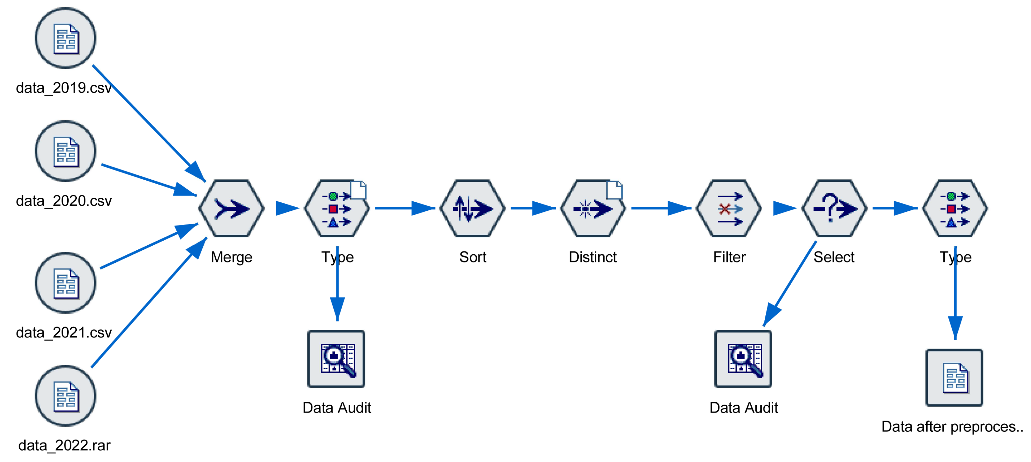
The SPSS modeler was used for all data preprocessing steps. It is a leading visual data science and machine learning solution designed by IBM. This helps enterprises accelerate the time to value by speeding up operational tasks for data scientists. Organizations worldwide use it for data preparation and discovery, predictive analytics, model management and deployment, and ML to monetize data assets [50,51]. The data preprocessing stream is illustrated in Figure 6.

Removal of duplicates: Duplicate data most often occur during the data collection process. This issue typically occurs when combining data from multiple sources or when receiving data from clients or multiple departments. A distinct node is employed to find or remove duplicate records from the dataset.

Fixing spelling and syntax errors: Some records contained syntax errors that were discovered when using the SPSS statistical data analysis tool. These records were modified to the correct values. For example, “2019” was discovered to be written incorrectly in the 2019 files and was changed from “201” to “2019”.

Handling missing values: A data audit node was used to report the data statistics depending on the field measurement levels. For categorical fields, the data audit reported the number of unique values (number of different categories). For continuous fields, the most important statistics were the minimum and maximum values because these criteria made it easy to detect out-of-range values. There are different methods for dealing with missing values, such as imputing or discarding them. Choosing the best technique depends on the size of the dataset, the number of fields containing blanks, and the amount of missing information. In this study, records with invalid values were discarded [49]. The number of removed duplicates and data with missing values was 78,609 records. The remaining data after data cleaning comprised 26,005,420 records. More details regarding the distribution of eliminated data are presented in Table 3.

Identifying and eliminating outliers: An outlier is another type of data anomaly that requires attention during the cleaning process. Outliers are data records that do not conform to the overall data distribution [52]. The mean and standard deviation of consumption for each month were computed. Typically, a threshold of three times the mean was used to mark the outliers. An outlier was said to be extreme if it was more than five standard deviations from the mean. Records with outliers or extremes were discarded because their numbers were very small relative to the dataset size.

Feature selection: This process involves choosing the input variables that have the strongest relationships with the target variable. This aids in creating an accurate predictive model. It can be used to identify and eliminate redundant, unnecessary, and irrelevant attributes from data that do not contribute to the model.

One of the commonly used methods for dimensionality reduction is principal component analysis. It helps in identifying the relationships among different variables and performs orthogonal transformations to convert them into a set of linearly correlated features [53]. Dimensionality reduction refers to the technique of reducing the dimensions of a training dataset by transforming high-dimensional data into a lower-dimensional space. The higher the number of features in a dataset, the more difficult it is to visualize and work on [54]. PCA can be classified into two categories:

• Feature selection: This is used to maintain the high accuracy of a model by carefully choosing the relevant features and eliminating all others.
• Feature extraction: This is used to identify new features in data after transforming them from a high-dimensional space to a low-dimensional space.

The difference between feature selection and extraction is that feature selection maintains a subset of the original features, whereas feature extraction creates new features [55].

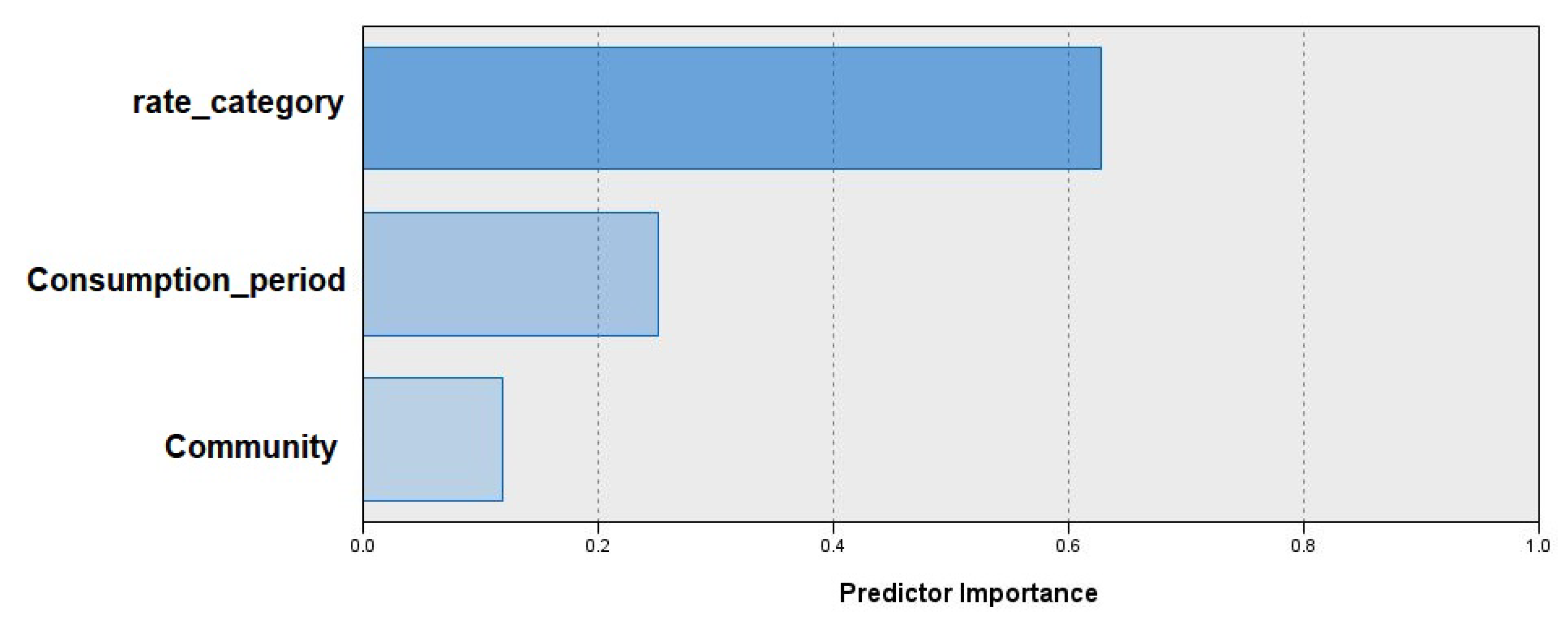
As shown in Figure 7, we used PCA as a feature selection technique that determined the weight of each predictor. The results revealed that the most important predictors were $rate\_category$, $consumption\_period$, and $community$; other input fields were filtered out by using the filter node.

Sampling: This was used to improve the performance and reduce the time consumption of the algorithm. The models generated from the samples were frequently as accurate as those obtained from the full dataset. In this study, two different sample types were used: a random sample and a sample that was stratified by using the SPSS sample node.

3. Results and Discussion

The main objective of forecasting electricity consumption is to determine the demand for the next month’s municipal areas in Dubai. Utility industry decision makers can anticipate future power consumption with the lowest possible error rate and future scaling of the grid by adding new power stations to high-demand regions.

3.1. MLR, RF, and ANN Performance Evaluation

Three machine learning techniques (MLR, RF, and ANN) were applied to the same dataset for a comparison based on their performance.

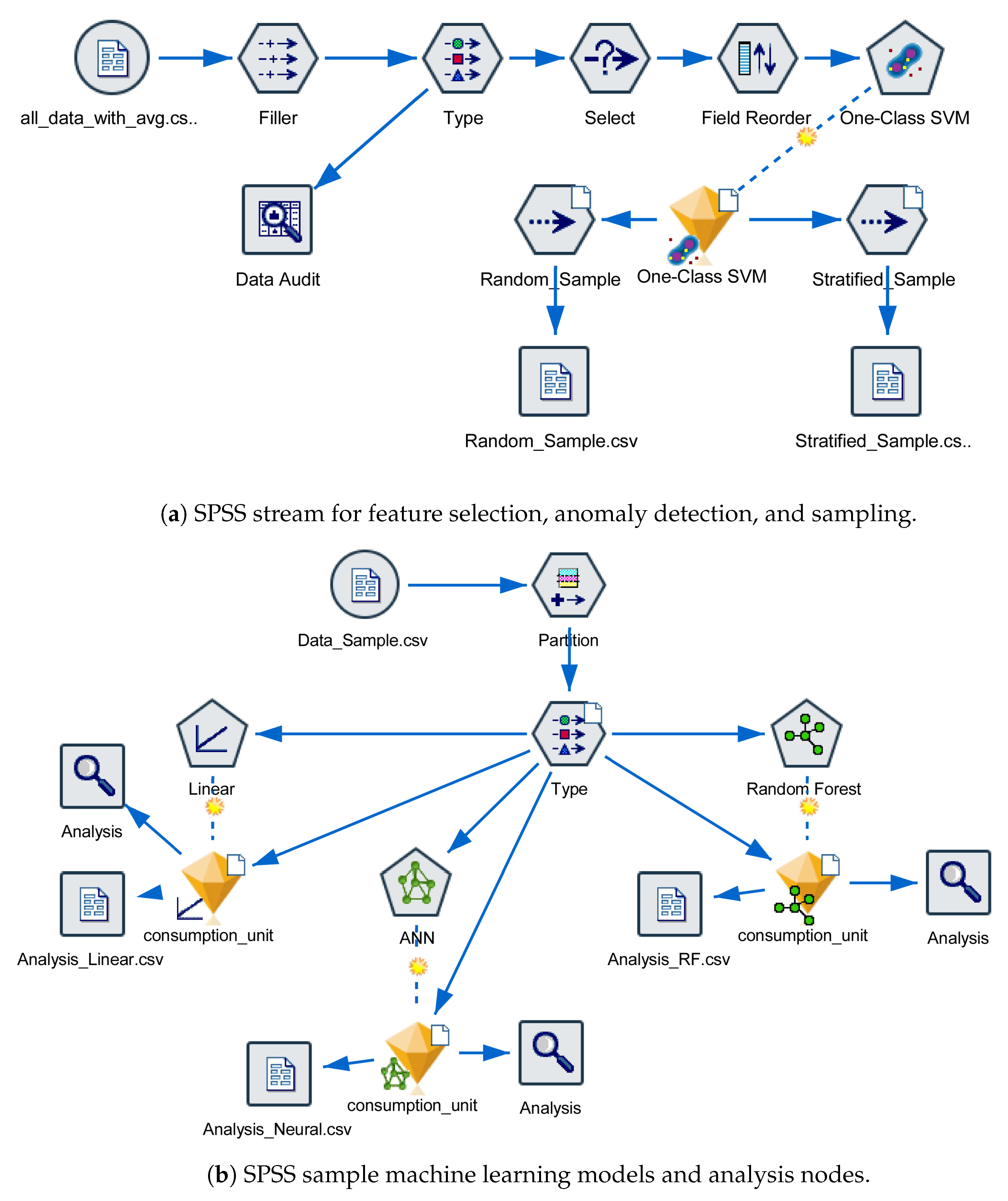
Figure 8 shows a graph of the entire SPSS flow, which includes the streams for all 12 scenarios. Scenarios 1, 2, and 3 used the original dataset and a random sampling method. Scenarios 4, 5, and 6 used the original dataset and a stratified sampling method.

According to

Table 4. Comparative accuracies of the training and testing models of different algorithms on both the original and enhanced dataset.

		Original Dataset			Enhanced Dataset
Sample	Type	Linear Regression	Neural	Random Forest	Linear Regression	Neural	Random Forest
Stratified	Training	46%	48.7%	66.3%	92%	97.5%	98.5%
	Testing	45.5%	47.9%	59.6%	91.9%	97.4%	97.1%
Random	Training	46%	49.1%	66.4%	90.6%	97.5%	98.5%
	Testing	45.9%	48.7%	60.5%	90.7%	97.4%	97.1%

, the accuracy of the original prediction was poor. Our work focused on enhancing the accuracy by using two steps: first, eliminating anomaly values from the dataset and then adding the influence of the weather to the model.

Anomaly detection involves observing abnormal status/events/entities that deviate from the majority of the system when they occur [56]. Anomaly detection methodologies can be divided into three categories: supervised, unsupervised, and semi-supervised [57]. To improve the prediction accuracy, we performed anomaly detection based on the one-class SVM algorithm, which can find abnormal consumption values in a dataset before model training. One-class SVM is an unsupervised algorithm. It classifies data into a single category. A decision boundary is first learned by using the characteristics of the normal samples of data, and then the anomalous data are identified and eliminated when they exceed this boundary. One-class SVM was implemented in Python with the scikit-learn version 1.1.3 library. Figure 9 shows that the one-class SVM had a clear boundary and labeled the data points outside of the boundary as anomalies that accounted for 2% of the sample dataset.

According to previous studies [58,59,60], weather fluctuations in temperature, humidity, wind, and precipitation significantly affect energy usage in the residential sector. This effect is typically measured in terms of the energy demand for cooling and heating. The agreement is that very hot temperatures reduce the electricity consumption for heating and increase the electricity consumption for cooling, and vice versa.

This dataset lacks the existence of weather data. To handle this, a new variable was added to the dataset, “$average\_consumption\_unit$ ($C{P}_{avg}$)”, which is the average power consumption for the three previous months to represent the consumption over one season. The added field was used to improve the correlation between the month of the year and the average power consumption.

$$C{P}_{{avg}_n}=\frac{C{P}_{n-1}+C{P}_{n-2}+C{P}_{n-3}}{3}$$

(12)

The other six scenarios (7)–(12) repeated the previous scenarios after anomaly elimination and with the newly added field $C{P}_{avg}$.

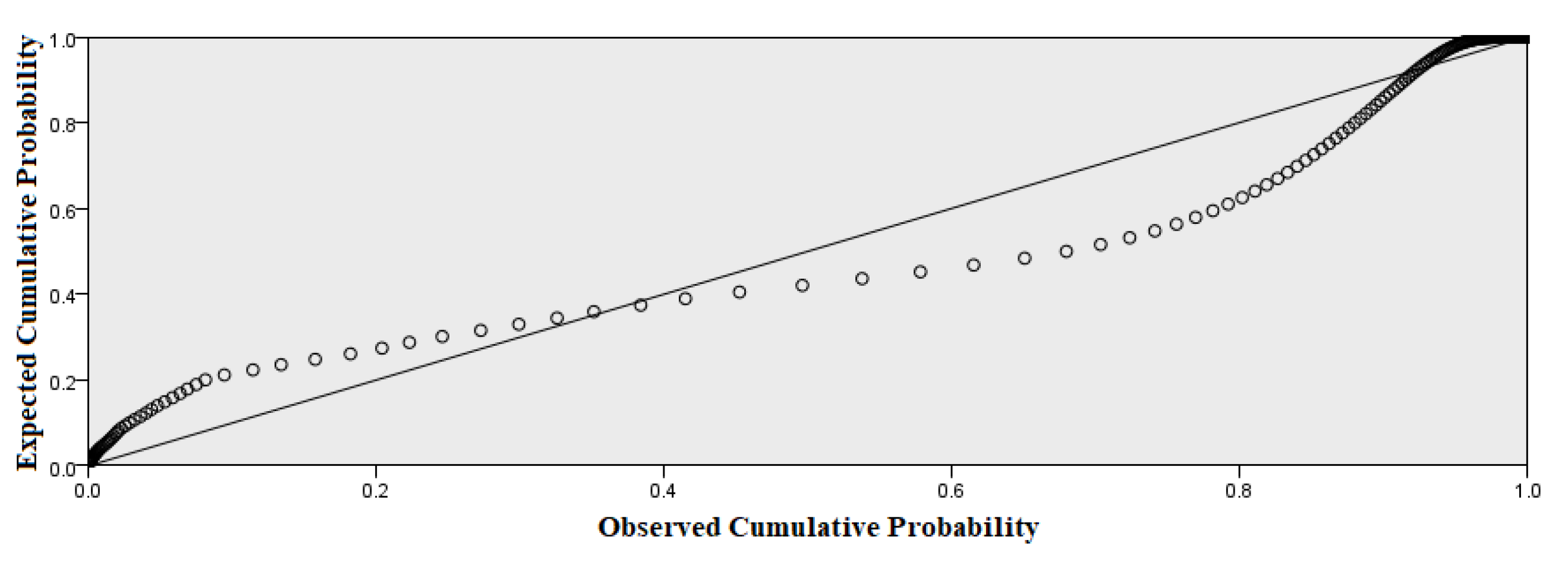
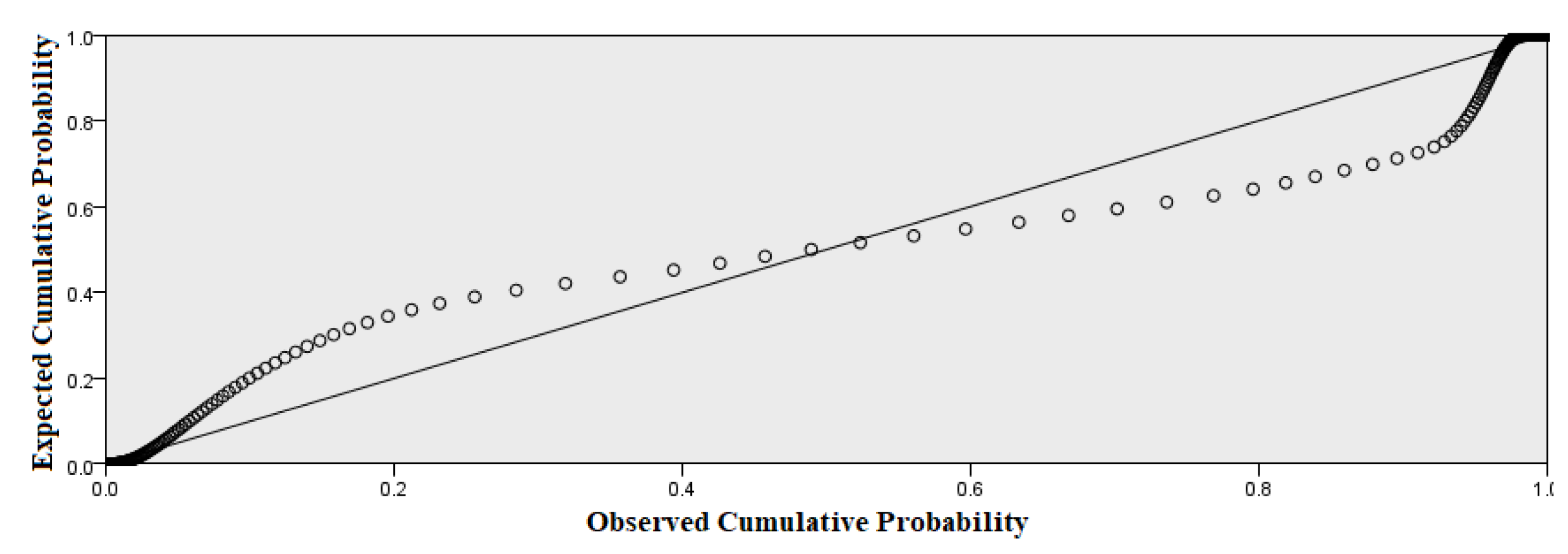
For MLR, Figure 10 and Figure 11 present the residual analysis of the linear regression, which shows the distance between the actual and predicted values. This refers to the difference between the observed and predicted values of electricity—“$consumption\_unit$”. To ensure that the model’s prediction line was, on average, as close to the actual values as possible, we aimed for the minimum residual standard error when the newly added field was used.

As shown in Figure 11, the performance was improved by using $C{P}_{avg}$; however, it was noted that many of the points were below the line and did not perfectly flow through each of the points. MLR did not achieve good results for this dataset because of the assumption of a simple and non-universally applicable straight-line relationship between the dependent and independent variables.

In the RF, we found the best values of $N\_estimators$, $Max\_depth$, $Minimum\_leaf\_size$, and $Max\_features$ by using a trial-and-error mechanism. From the results, it was found that although using a large number of trees was better, it could take a long time to compute. In addition, it should be noted that the results would plateau after a certain number of trees and stop improving considerably. Using a lower number of features reduced the variance, but would also lead to a greater increase in bias. Empirically good results were frequently obtained by combining $Max\_features$ = sqrt (using a random subset of size sqrt(n_features)), $Max\_depth$ = None, and $Minimum\_leaf\_samples$ = 2.

For the ANN, the prediction was performed by using a typical neural network with one hidden layer. The number of hidden neurons was selected by using a trial-and-error method. In this work, 5, 7, 10, 16, and 32 neurons were used. The best model accuracy was achieved by using 32 neurons.

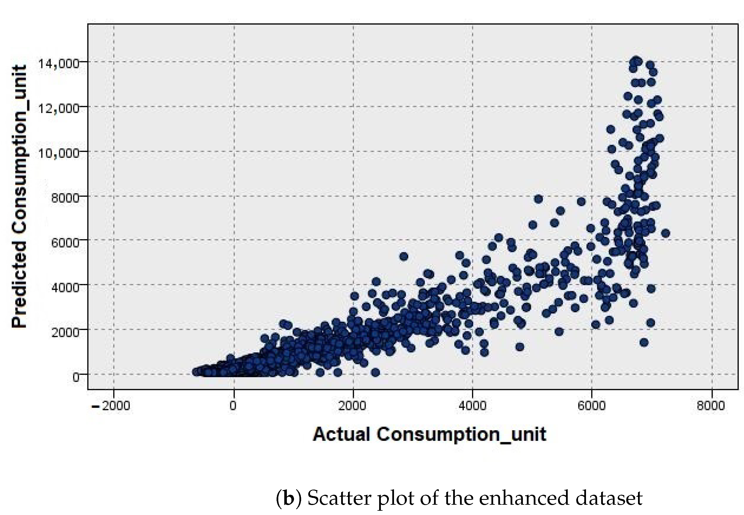
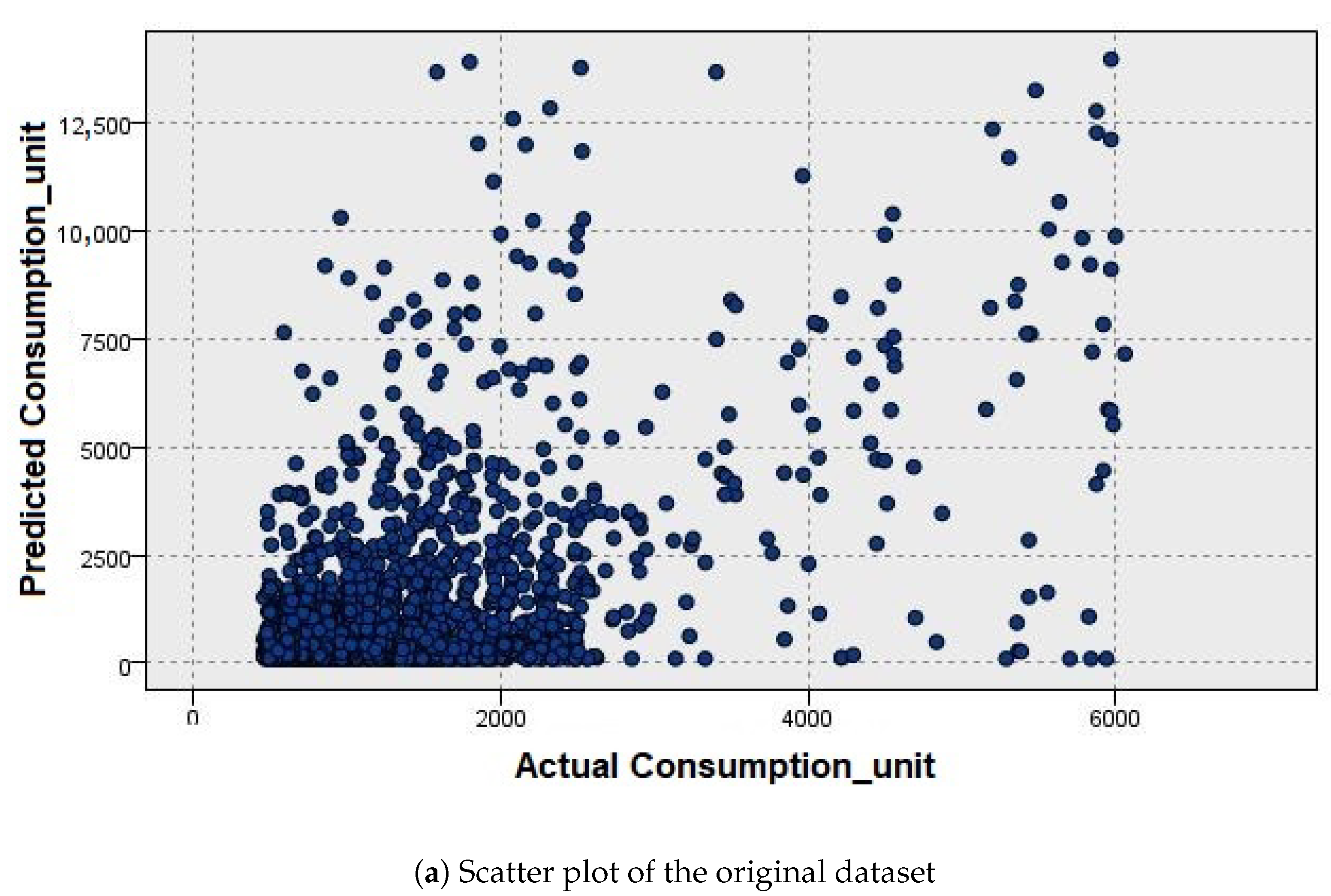
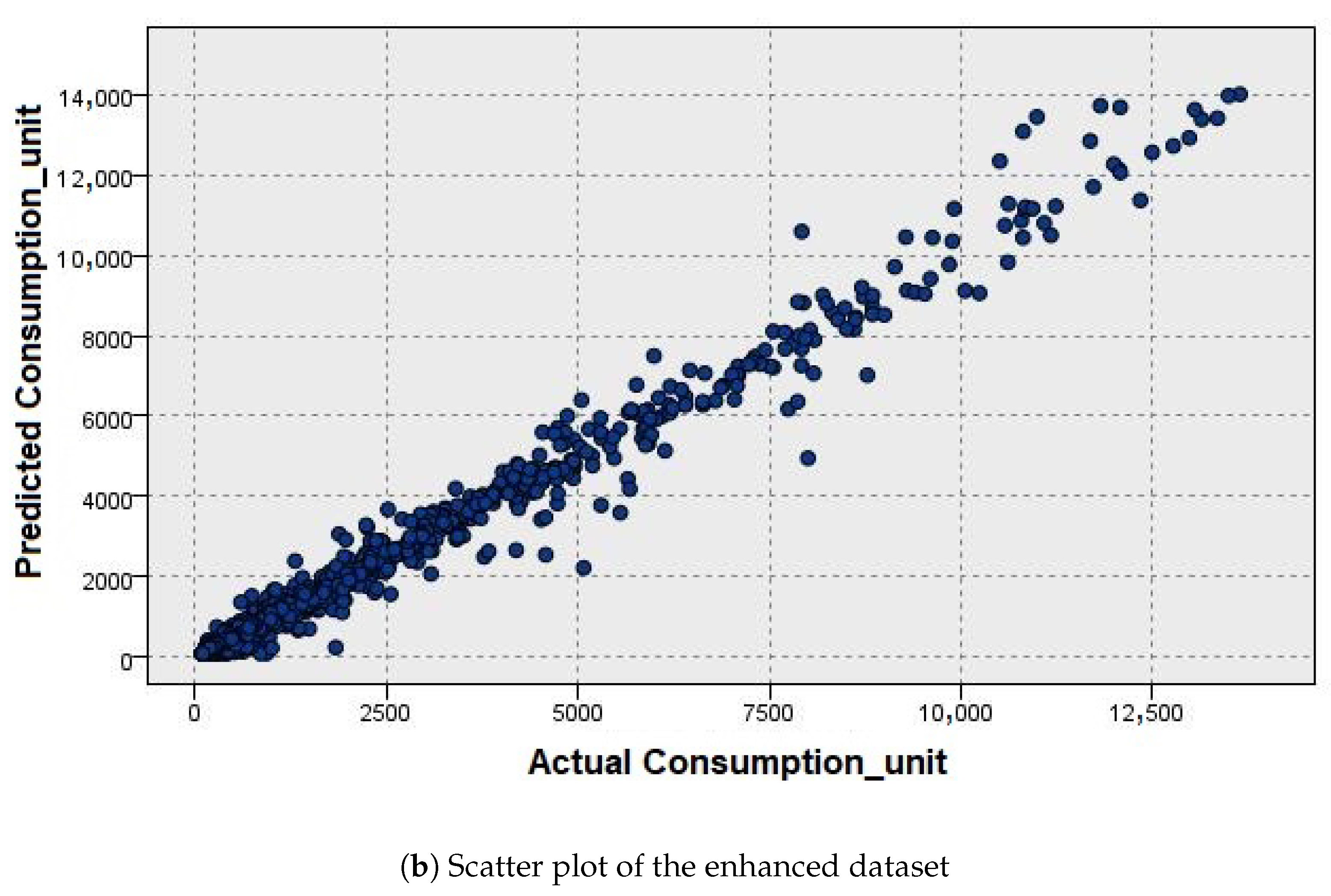
Scatter plots are frequently used to show the relationship between actual and predicted values and to observe the nature of a relationship. The horizontal axis is the actual consumption unit, and the vertical axis is the forecast consumption unit, as illustrated in Figure 12, Figure 13 and Figure 14. The results in part (a) demonstrate that the shape was nonlinear, with a weak association in the original dataset. After using the newly added field ($C{P}_{avg}$), the data appeared to be linearly related, and the spread of the data was similar across the regression line, which achieved the homoscedasticity and linearity assumptions.

The performance of the three algorithms was validated by comparing the obtained results by using four statistical parameter values: the root mean square error (RMSE), mean absolute percentage error (MAPE), mean absolute error (MAE), and correlation coefficient ($R^2$), as well as the processing time [61]. Their values were calculated by using Python code after exporting the predicted output values from the SPSS program. The calculated values are presented in

Table 5. Evaluation metrics of the trained machine learning models on both the original and enhanced dataset.

		Original Dataset				Enhanced Dataset
Sample	Algorithm	MAPE	MAE	RMSE	R${}^{\mathbf{2}}$	MAPE	MAE	RMSE	R${}^{\mathbf{2}}$
	Linear	2.79	1182.49	1935.78	0.19	0.75	481.56	936.79	0.81
Stratified	Neural	2.77	1159.78	1908.53	0.215	0.31	229.06	513.51	0.943
	Random Forest	2.14	954.61	1674.28	0.396	0.157	131.44	333.04	0.976
	Linear	2.79	1184.32	1939.06	0.191	0.739	466.45	908.08	0.822
Random	Neural	2.761	1160.58	1911.2	0.214	0.328	221.51	488.1	0.948
	Random Forest	2.14	956.39	1679.46	0.393	0.158	132.98	338.36	0.975

.

$$RMSE=\sqrt{\frac{1}{n}\sum _{i=1}^n{(y_i-{\widehat{y}}_i)}^2}$$

(13)

$$MAE=\frac{1}{n}\sum _{i=1}^n|y_i-{\widehat{y}}_i|$$

(14)

$$MAPE=\frac{100\%}{n}\sum _{i=1}^n|\frac{y_i-{\widehat{y}}_i}{y_i}|$$

(15)

$$R^2=1-\frac{{\sum }_{i=1}^n{(y_i-{\widehat{y}}_i)}^2}{{\sum }_{i=1}^n{(y_i-{\overline{y}}_i)}^2}$$

(16)

where y is the actual value, $\widehat{y}$ is the predicted value, and $\overline{y}$ is the mean value.

Table 4 provides a comparison of the accuracies obtained from the different models. Working with the original dataset resulted in poor performance, with an accuracy of 66% in the best case. When using the $C{P}_{avg}$ field, both the ANN and RF achieved excellent accuracy. The RF was slightly better than the ANN.

Table 5 lists the values of the criteria used to estimate the prediction errors of the models. When comparing the performance of the models, it was observed that the forecast errors were higher when using MLR, which made it inappropriate for this dataset. The RF performed better than the ANN in terms of the MAPE, MAE, RMSE, and $R^2$ values. The model building and prediction times of the three algorithms are listed in

Table 6. Model building and prediction times (in seconds) of different algorithms on both the original and enhanced dataset.

		Original Dataset		Enhanced Dataset
Sample	Algorithm	Model Building (s)	Prediction (s)	Model Building (s)	Prediction (s)
	Linear	12	7	14	8
Stratified	Neural	158	7	569	7
	Random Forest	37	980	85	987
	Linear	9	7.3	11	7.9
Random	Neural	179	6.7	617	7
	Random Forest	40	953	71	978

. The ANN required a longer time than the RF to build the model, while the ANN had a much faster prediction time than that of the RF.

The results indicate that, in most cases, using an ANN is recommended for such data types, particularly when dealing with a complete dataset, for several reasons:

• The accuracy is almost the same between an ANN and RF.
• An ANN has a significantly lower prediction time than that of an RF.

Additionally, when concentrating on a single categorical area, such as a residential area, the ANN performed better than the RF, with an accuracy of 91.02%. When applied to a single residential customer, both models attained the same accuracy (90.01%).

3.2. ARIMA Performance Evaluation

ARIMA time-series analysis was also considered for several reasons. It is simple to use and suitable for a wide range of data. It is also relatively accurate, and it can be used to forecast long-term trends. However, ARIMA has certain limitations. It is not always accurate and can be difficult to interpret. A large amount of data is also required for it to be effective [62].

ARIMA was applied to the entire dataset in three different scenarios. Scenario 1 was used to predict the future consumption of Dubai. Scenario 2 was applied to a single area to predict district loads and provide insights into capacity expansion. Scenario 3 was used for individual customers to predict specific customer consumption and send notifications as required [63].

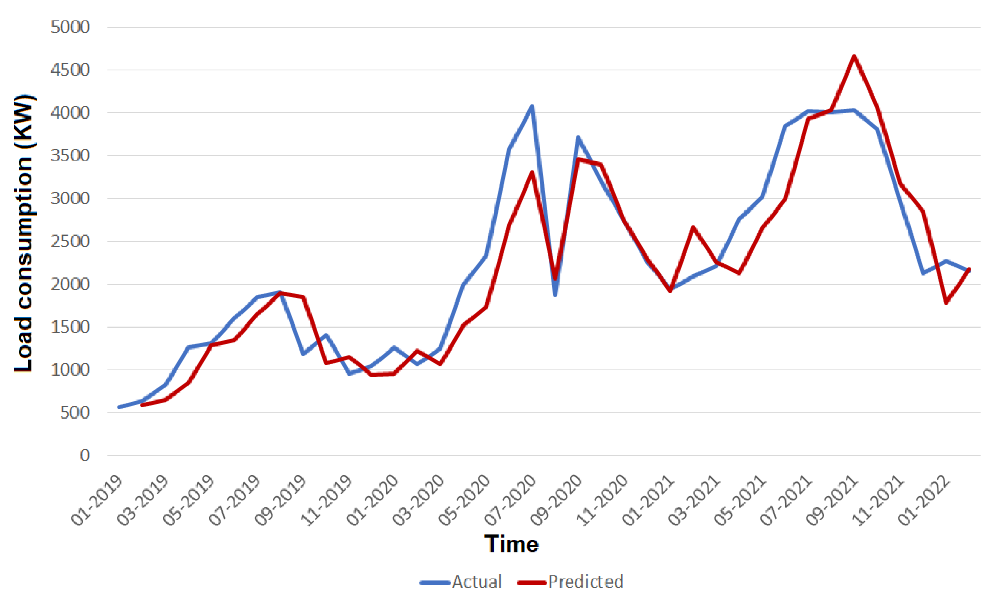
For each scenario, the actual and predicted consumption was plotted against time to demonstrate the prediction performance. As shown in Figure 15, the prediction performance was outstanding in the beginning, but did not achieve the same performance in 2020. Figure 16 illustrates that the best ARIMA performance was achieved by forecasting one district scenario. Poor results were obtained when ARIMA was used to predict single-user consumption, as shown in Figure 17.

Table 7. Evaluation metrics of the ARIMA model on the DEWA dataset for different scenarios.

Scenario	MAPE	MAE	RMSE	R${}^2$	Accuracy
ARIMA, whole of Dubai	28	813	1114.1	0.575	78%
ARIMA, one district	14	307	414.5	0.85	93%
ARIMA, one customer	66	307	410	0.42	71%

lists the performance of the three scenarios based on the MAPE, MAE, RMSE, $R^2$, and accuracy. This Table demonstrates that ARIMA can be used to predict future district consumption. Because of the poor values of the accuracy and prediction error in scenarios 1 and 3, ARIMA is not recommended in these cases.

4. Conclusions and Future Work

Electricity load forecasting is one of the important considerations in operating a nation’s electric power system. In this study, we focused on selecting an appropriate machine learning technique for the LTLF in Dubai to assist smart utility companies by saving power and reducing costs. The electricity demands of the different categories were predicted, and the total demand for the entire country was obtained. This study focused on the DEWA dataset because of the lack of research focusing on the consumption behavior of this region (Middle Eastern countries).

The steps of the methodology are summarized as follows: The first stage was data preprocessing, which included eliminating or modifying incorrect, missing, irrelevant, duplicated, or improperly formatted data to prepare for the analysis. PCA was used as a feature selection technique that determined the weight of each predictor and chose the most revealing predictors that affected our study. Sampling was used to improve the performance and reduce the time required to run the algorithms.

In the second stage, MLR, RF, and ANN were used for load prediction by using the original dataset. The results showed that the accuracies were approximately 46%, 48.7%, and 66.3% for MLR, ANN, and RF, respectively.

The third stage included our method of enhancing the prediction accuracy by detecting anomaly values with one-class SVM. A decision boundary was first learned by using the characteristics of the normal samples of data, and then the anomalous data were identified and eliminated when they exceeded this boundary. In addition, we added a new variable, “$C{P}_{avg}$”, to mimic the influence of the weather on the model, as the dataset lacked the inclusion of weather data. This represented the consumption in one season. Repeating the prediction, the results showed that the performance was significantly enhanced after anomaly elimination and the use of the proposed field.

In addition, ARIMA was applied to the entire dataset after anomaly illumination in three different scenarios: predicting the future consumption of the entirety of Dubai, predicting that of a single area in order to predict district loads, and predicting specific customers’ consumption. The results showed that the best accuracy of ARIMA was approximately 93% when working in only a single district.

The results showed that both the ANN and RF achieved an excellent accuracy of approximately 97%. Therefore, the use of an ANN for such data types is recommended in most cases, particularly when working on a whole country, for several reasons—the accuracy is almost the same between an ANN and RF, and an ANN has a significantly lower prediction time than that of an RF.

Furthermore, when working on a single categorical area, both the ANN and RF models were good choices because they achieved the same accuracy of approximately 91.02%.

Future work will concentrate on including real weather data to study seasonal fluctuations that affect consumer behavior and load usage, using anomaly detection and prediction data to identify abnormal events in consumption, such as theft, metering malfunctions, and technical losses, and developing a program for revealing customers’ current and expected usage.

References

1. Lloret, J.; Tomas, J.; Canovas, A.; Parra, L. An integrated IoT architecture for smart metering. IEEE Commun. Mag. 2016, 54, 50–57. [Google Scholar] [CrossRef]
2. Dileep, G. A survey on smart grid technologies and applications. Renew. Energy 2020, 146, 2589–2625. [Google Scholar] [CrossRef]
3. Suresh, M.; Anbarasi, M.; Jayasre, R.; Shivani, C.; Sowmiya, P. Smart Meter Data Analytics Using Particle Swarm Optimization. In Proceedings of the 2019 IEEE International Conference on System, Computation, Automation and Networking (ICSCAN), Pondicherry, India, 29–30 March 2019; pp. 1–5. [Google Scholar]
4. Joy, J.; Jasmin, E.; John, V.R. Challenges of smart grid. Int. J. Adv. Res. Electr. Electron. Instrum. Eng. 2013, 2, 976–981. [Google Scholar]
5. Davoody-Beni, Z.; Sheini-Shahvand, N.; Shahinzadeh, H.; Moazzami, M.; Shaneh, M.; Gharehpetian, G.B. Application of IoT in smart grid: Challenges and solutions. In Proceedings of the 2019 5th iranian conference on signal processing and intelligent systems (ICSPIS), Shahrood, Iran, 18–19 December 2019; pp. 1–8. [Google Scholar]
6. Khan, M.Z.; Alhazmi, O.H.; Javed, M.A.; Ghandorh, H.; Aloufi, K.S. Reliable Internet of Things: Challenges and future trends. Electronics 2021, 10, 2377. [Google Scholar] [CrossRef]
7. Völker, B.; Reinhardt, A.; Faustine, A.; Pereira, L. Watt’s up at home? Smart meter data analytics from a consumer-centric perspective. Energies 2021, 14, 719. [Google Scholar] [CrossRef]
8. Amin, P.; Cherkasova, L.; Aitken, R.; Kache, V. Analysis and demand forecasting of residential energy consumption at multiple time scales. In Proceedings of the 2019 IFIP/IEEE Symposium on Integrated Network and Service Management (IM), Washington, DC, USA, 9–11 April 2019; pp. 494–499. [Google Scholar]
9. Zhou, F.; Wen, G.; Ma, Y.; Geng, H.; Huang, R.; Pei, L.; Yu, W.; Chu, L.; Qiu, R. A Comprehensive Survey for Deep-Learning-Based Abnormality Detection in Smart Grids with Multimodal Image Data. Appl. Sci. 2022, 12, 5336. [Google Scholar] [CrossRef]
10. Sahoo, S.; Nikovski, D.; Muso, T.; Tsuru, K. Electricity theft detection using smart meter data. In Proceedings of the 2015 IEEE Power & Energy Society Innovative Smart Grid Technologies Conference (ISGT), Washington, DC, USA, 18–20 February 2015; pp. 1–5. [Google Scholar]
11. He, Z.; Zhao, C.; Huang, Y. Multivariate Time Series Deep Spatiotemporal Forecasting with Graph Neural Network. Appl. Sci. 2022, 12, 5731. [Google Scholar] [CrossRef]
12. Sulaiman, S.; Jeyanthy, P.A.; Devaraj, D.; Mohammed, S.S.; Shihabudheen, K. Smart meter data analytics for load prediction using extreme learning machines and artificial neural networks. In Proceedings of the 2019 IEEE International Conference on Clean Energy and Energy Efficient Electronics Circuit for Sustainable Development (INCCES), Krishnankoil, India, 18–20 December 2019; pp. 1–4. [Google Scholar]
13. Mohan, S.K.; John, A.; Padmanaban, S.; Hamid, Y. Hybrid Intelligent Approaches for Smart Energy: Practical Applications; John Wiley & Sons: Hoboken, NJ, USA, 2022. [Google Scholar]
14. Al Mamun, A.; Sohel, M.; Mohammad, N.; Sunny, M.S.H.; Dipta, D.R.; Hossain, E. A comprehensive review of the load forecasting techniques using single and hybrid predictive models. IEEE Access 2020, 8, 134911–134939. [Google Scholar] [CrossRef]
15. Jiang, Y.; Gao, T.; Dai, Y.; Si, R.; Hao, J.; Zhang, J.; Gao, D.W. Very short-term residential load forecasting based on deep-autoformer. Appl. Energy 2022, 328, 120120. [Google Scholar] [CrossRef]
16. Matrenin, P.; Safaraliev, M.; Dmitriev, S.; Kokin, S.; Ghulomzoda, A.; Mitrofanov, S. Medium-term load forecasting in isolated power systems based on ensemble machine learning models. Energy Rep. 2022, 8, 612–618. [Google Scholar] [CrossRef]
17. Carvallo, J.P.; Larsen, P.H.; Sanstad, A.H.; Goldman, C.A. Long term load forecasting accuracy in electric utility integrated resource planning. Energy Policy 2018, 119, 410–422. [Google Scholar] [CrossRef]
18. Zhang, P.; Wu, X.; Wang, X.; Bi, S. Short-term load forecasting based on big data technologies. CSEE J. Power Energy Syst. 2015, 1, 59–67. [Google Scholar] [CrossRef]
19. Shaban, M.; Alsharekh, M.F. Design of a Smart Distribution Panelboard Using IoT Connectivity and Machine Learning Techniques. Energies 2022, 15, 3658. [Google Scholar] [CrossRef]
20. Memarzadeh, G.; Keynia, F. Short-term electricity load and price forecasting by a new optimal LSTM-NN based prediction algorithm. Electr. Power Syst. Res. 2021, 192, 106995. [Google Scholar] [CrossRef]
21. Zhang, G.; Bai, X.; Wang, Y. Short-time multi-energy load forecasting method based on CNN-Seq2Seq model with attention mechanism. Mach. Learn. Appl. 2021, 5, 100064. [Google Scholar] [CrossRef]
22. Lee, Y.J.; Choi, H.J. Forecasting building electricity power consumption using deep learning approach. In Proceedings of the 2020 IEEE International Conference on Big Data and Smart Computing (BigComp), Pusan, Republic of Korea, 19–22 February 2020; pp. 542–544. [Google Scholar]
23. Jeyaranjani, J.; Devaraj, D. Deep learning based smart meter data analytics for electricity load prediction. In Proceedings of the 2019 IEEE International Conference on Clean Energy and Energy Efficient Electronics Circuit for Sustainable Development (INCCES), Krishnankoil, India, 18–20 December 2019; pp. 1–5. [Google Scholar]
24. Atef, S.; Eltawil, A.B. Real-time load consumption prediction and demand response scheme using deep learning in smart grids. In Proceedings of the 2019 6th International Conference on Control, Decision and Information Technologies (CoDIT), Paris, France, 23–26 April 2019; pp. 1043–1048. [Google Scholar]
25. Chandramitasari, W.; Kurniawan, B.; Fujimura, S. Building deep neural network model for short term electricity consumption forecasting. In Proceedings of the 2018 International Symposium on Advanced Intelligent Informatics (SAIN), Yogyakarta, Indonesia, 29–30 August 2018; pp. 43–48. [Google Scholar]
26. Pannakkong, W.; Harncharnchai, T.; Buddhakulsomsiri, J. Forecasting Daily Electricity Consumption in Thailand Using Regression, Artificial Neural Network, Support Vector Machine, and Hybrid Models. Energies 2022, 15, 3105. [Google Scholar] [CrossRef]
27. Ma, Y.J.; Zhai, M.Y. Day-ahead prediction of microgrid electricity demand using a hybrid artificial intelligence model. Processes 2019, 7, 320. [Google Scholar] [CrossRef] [Green Version]
28. Masum, A.K.M.; Chy, M.K.A.; Hasan, M.T.; Sayeed, M.H.; Reza, S.T. Smart meter with load prediction feature for residential customers in Bangladesh. In Proceedings of the 2019 International Conference on Energy and Power Engineering (ICEPE), Dhaka, Bangladesh, 14–16 March 2019; pp. 1–6. [Google Scholar]
29. Mariano-Hernández, D.; Hernández-Callejo, L.; Solís, M.; Zorita-Lamadrid, A.; Duque-Pérez, O.; Gonzalez-Morales, L.; García, F.S.; Jaramillo-Duque, A.; Ospino-Castro, A.; Alonso-Gómez, V.; et al. Analysis of the Integration of Drift Detection Methods in Learning Algorithms for Electrical Consumption Forecasting in Smart Buildings. Sustainability 2022, 14, 5857. [Google Scholar] [CrossRef]
30. Jahić, A.; Konjić, T.; Hivziefendić, J. Detection of missing power meter readings using artificial neural networks. In Proceedings of the 2017 XXVI International Conference on Information, Communication and Automation Technologies (ICAT), Sarajevo, Bosnia and Herzegovina, 26–28 October 2017; pp. 1–6. [Google Scholar]
31. Liu, M.; Liu, D.; Sun, G.; Zhao, Y.; Wang, D.; Liu, F.; Fang, X.; He, Q.; Xu, D. Deep learning detection of inaccurate smart electricity meters: A case study. IEEE Ind. Electron. Mag. 2020, 14, 79–90. [Google Scholar] [CrossRef]
32. Wanxing, S.; Keyan, L.; Huanna, N.; Yuzhu, W.; Jingxiang, Z. The anomalous data identification study of reactive power optimization system based on big data. In Proceedings of the 2016 International Conference on Probabilistic Methods Applied to Power Systems (PMAPS), Beijing, China, 16–20 October 2016; pp. 1–5. [Google Scholar]
33. Amara korba, A.; El Islem karabadji, N. Smart Grid Energy Fraud Detection Using SVM. In Proceedings of the 2019 International Conference on Networking and Advanced Systems (ICNAS), Annaba, Algeria, 26–27 June 2019; pp. 1–6. [Google Scholar] [CrossRef]
34. Liu, F.; Liang, C.; He, Q. Remote malfunctional smart meter detection in edge computing environment. IEEE Access 2020, 8, 67436–67443. [Google Scholar] [CrossRef]
35. Canepa, G. What You Need to Know about Machine Learning; Packt Publishing: Birmingham, UK, 2016. [Google Scholar]
36. Müller, A.C.; Guido, S. Introduction to Machine Learning with Python: A Guide for Data Scientists; O’Reilly Media, Inc.: Sebastopol, CA, USA, 2016. [Google Scholar]
37. Harrington, P. Machine Learning in Action; Simon and Schuster: New York, NY, USA, 2012. [Google Scholar]
38. Fitzek, F.; Granelli, F.; Seeling, P. Computing in Communication Networks: From Theory to Practice; Academic Press: Cambridge, MA, USA, 2020. [Google Scholar]
39. Montgomery, D.C.; Peck, E.A.; Vining, G.G. Introduction to Linear Regression Analysis; John Wiley & Sons: Hoboken, NJ, USA, 2021. [Google Scholar]
40. Uyanık, G.K.; Güler, N. A study on multiple linear regression analysis. Procedia-Soc. Behav. Sci. 2013, 106, 234–240. [Google Scholar] [CrossRef] [Green Version]
41. Pujara, P.; Chaudhari, M. Phishing website detection using machine learning: A review. Int. J. Sci. Res. Comput. Sci. Eng. Inf. Technol. 2018, 3, 395–399. [Google Scholar]
42. Breiman, L. Random forests. Mach. Learn. 2001, 45, 5–32. [Google Scholar] [CrossRef] [Green Version]
43. Kartelj, A.; Kotlar, M. (Eds.) Implementation of Machine Learning Algorithms Using Control-Flow and Dataflow Paradigms; IGI Global: Hershey, PA, USA, 2022. [Google Scholar]
44. Biau, G. Analysis of a random forests model. J. Mach. Learn. Res. 2012, 13, 1063–1095. [Google Scholar]
45. Bell, J. Machine Learning: Hands-On for Developers and Technical Professionals; John Wiley & Sons: Hoboken, NJ, USA, 2020. [Google Scholar]
46. Ahamed, K.; Akthar, S. Survey on artificial neural network learning technique algorithms. Int. Res. J. Eng. Technol. 2016, 3, 36–39. [Google Scholar]
47. Chen, M.; Challita, U.; Saad, W.; Yin, C.; Debbah, M. Artificial neural networks-based machine learning for wireless networks: A tutorial. IEEE Commun. Surv. Tutor. 2019, 21, 3039–3071. [Google Scholar] [CrossRef] [Green Version]
48. Dubai Consumption Dataset Link. Available online: https://www.dubaipulse.gov.ae/organisation/dewa/service/dewa-consumption (accessed on 5 March 2022).
49. Han, J.; Pei, J.; Tong, H. Data Mining: Concepts and Techniques; Morgan Kaufmannp: San Francisco, CA, USA, 2022. [Google Scholar]
50. Wendler, T.; Gröttrup, S. Data Mining with SPSS Modeler: Theory, Exercises and Solutions; Springer: Berlin/Heidelberg, Germany, 2016. [Google Scholar]
51. Nasir, M.A.; Bakouch, H.S.; Jamal, F. Introductory Statistical Procedures with SPSS; Bentham Science Publishers: Sharjah, United Arab Emirates, 2022. [Google Scholar]
52. Abdallah, Z.S.; Du, L.; Webb, G.I. Data Preparation. In Encyclopedia of Machine Learning and Data Mining; Sammut, C., Webb, G.I., Eds.; Springer: Boston, MA, USA, 2017; pp. 318–327. [Google Scholar] [CrossRef]
53. Vidal, R.; Ma, Y.; Sastry, S.S. Principal component analysis. In Generalized Principal Component Analysis; Springer: Berlin/Heidelberg, Germany, 2016; pp. 25–62. [Google Scholar]
54. Sano, N. Synthetic Data by Principal Component Analysis. In Proceedings of the 2020 International Conference on Data Mining Workshops (ICDMW), Sorrento, Italy, 17–20 November 2020; pp. 101–105. [Google Scholar]
55. Karamizadeh, S.; Abdullah, S.M.; Manaf, A.A.; Zamani, M.; Hooman, A. An overview of principal component analysis. J. Signal Inf. Process. 2020, 4, 173–175. [Google Scholar] [CrossRef] [Green Version]
56. Lin, X.X.; Lin, P.; Yeh, E.H. Anomaly detection/prediction for the Internet of Things: State of the art and the future. IEEE Netw. 2020, 35, 212–218. [Google Scholar] [CrossRef]
57. Tsai, C.W.; Chiang, K.C.; Hsieh, H.Y.; Yang, C.W.; Lin, J.; Chang, Y.C. Feature Extraction of Anomaly Electricity Usage Behavior in Residence Using Autoencoder. Electronics 2022, 11, 1450. [Google Scholar] [CrossRef]
58. Kang, J.; Reiner, D.M. What is the effect of weather on household electricity consumption? Empirical evidence from Ireland. Energy Econ. 2022, 111, 106023. [Google Scholar] [CrossRef]
59. Erba, S.; Causone, F.; Armani, R. The effect of weather datasets on building energy simulation outputs. Energy Procedia 2017, 134, 545–554. [Google Scholar] [CrossRef]
60. Gutiérrez González, V.; Ramos Ruiz, G.; Du, H.; Sánchez-Ostiz, A.; Fernández Bandera, C. Weather files for the calibration of building energy models. Appl. Sci. 2022, 12, 7361. [Google Scholar] [CrossRef]
61. Chai, T.; Draxler, R.R. Root mean square error (RMSE) or mean absolute error (MAE)?–Arguments against avoiding RMSE in the literature. Geosci. Model Dev. 2014, 7, 1247–1250. [Google Scholar] [CrossRef] [Green Version]
62. Contreras, J.; Espinola, R.; Nogales, F.J.; Conejo, A.J. ARIMA models to predict next-day electricity prices. IEEE Trans. Power Syst. 2003, 18, 1014–1020. [Google Scholar] [CrossRef]
63. Jagait, R.K.; Fekri, M.N.; Grolinger, K.; Mir, S. Load forecasting under concept drift: Online ensemble learning with recurrent neural network and ARIMA. IEEE Access 2021, 9, 98992–99008. [Google Scholar] [CrossRef]
Figure 1. Framework of the load forecasting model.
Electronics 12 00389 g001
Figure 2. Structure of an RF model with n trees.
Electronics 12 00389 g002
Figure 3. Structure of an ANN model with one hidden layer and seven neurons.
Electronics 12 00389 g003
Figure 4. Example of a PACF plot.
Electronics 12 00389 g004
Figure 5. Example of an ACF plot.
Electronics 12 00389 g005
Figure 6. Data preprocessing stream with SPSS.
Electronics 12 00389 g006
Figure 7. Feature selection using PCA.
Electronics 12 00389 g007
Figure 8. Stream components of the machine learning models in the SPSS Modeler.
Electronics 12 00389 g008
Figure 9. Anomaly detection graph created with the one-class SVM.
Electronics 12 00389 g009
Figure 10. Residual analysis of MLR.
Electronics 12 00389 g010
Figure 11. Residual analysis of MLR with C P a v g .
Electronics 12 00389 g011
Figure 12. Scatter plots showing the relationship between the actual and predicted power consumption values using MLR.
Electronics 12 00389 g012aElectronics 12 00389 g012b
Figure 13. Scatter plots showing the relationship between the actual and predicted power consumption values using the ANN.
Electronics 12 00389 g013aElectronics 12 00389 g013b
Figure 14. Scatter plots showing the relationship between the actual and predicted power consumption values using the RF.
Electronics 12 00389 g014aElectronics 12 00389 g014b
Figure 15. Actual and predicted load consumption values in MW versus time for the entirety of Dubai using the ARIMA model.
Electronics 12 00389 g015
Figure 16. Actual and predicted load consumption values in KW versus time for one district of Dubai using the ARIMA model.
Electronics 12 00389 g016
Figure 17. Actual and predicted load consumption values in W versus time for one customer using the ARIMA model.
Electronics 12 00389 g017