A Scalable Spatial–Temporal Correlated Non-Stationary Channel Fading Generation Method

Abstract

To address the challenges of complex implementation structures and high hardware resource consumption in multiple-input multiple-output (MIMO) channel emulators, this paper proposes a hardware generation method for spatial–temporal correlated non-stationary channel fading. Firstly, a hardware generation architecture is developed for field-programmable gate array (FPGA) platforms, which can also reduce the complexity of the channel emulator. Secondly, an improved CORDIC method is introduced to reduce algorithm latency and hardware consumption while expanding the function convergence domain, with a relative error maintained at the level of 10-4. Furthermore, based on the idea of time-division multiplexing, an efficient hardware operation of a lower triangular matrix is adopted to minimize the consumption of hardware resources. Finally, the measured results demonstrate that the statistical characteristics of the channel fading generated by the proposed method are in good agreement with the theoretical ones, with an average error of less than 2%. Additionally, under identical simulation conditions, hardware resource consumption is reduced by 6.87%. These findings provide compelling evidence of the enhanced efficiency and accuracy in simulating MIMO channels achieved through the proposed method.

1. Introduction

Multi-input multi-output (MIMO) technology is widely employed in wireless communications to effectively enhance channel capacity and frequency band utilization [1,2,3]. With advancements in antenna technology leading to miniaturization, MIMO communication systems are being applied in various communication scenarios [4,5,6]. However, diverse and complex propagation environments have a significant impact on system performance [7,8]. Research into optimizing the performance of MIMO communication systems has garnered significant attention [9,10,11]. Channel emulators provide a means to emulate the effects of real-world propagation environments on signals within a laboratory setting, aiding in the design, evaluation, and optimization of communication systems [12]. As the number of antennas increases and dynamic propagation environments become prevalent, existing channel emulators struggle to support massive and non-stationary MIMO channel emulations [13,14,15]. There is a growing need for the development of more efficient and accurate fading generation methods to address these challenges.

Currently, commercial channel emulators include Agilent’s N5106A PXB [16], Keysight’s propsim F64 [17], and Azimuth’s ACE 400WB [18]. Despite their good performance in generating standardized channel models, these emulators are both intricate in structure and financially burdensome. Furthermore, the simulation methods they used had limitations, which researchers had studied. The authors in [19] developed a non-stationary channel generation method on a software radio platform. However, this method was unsuitable for scenarios with fast-moving transceivers, because the generated Doppler frequencies were imprecise compared to the measurements. The sum-of-sinusoids (SoS) method proposed in [20,21,22] was suitable for the implementation of FPGA hardware platforms, but it suffered from a problem of phase discontinuity. In [23,24], the authors proposed the sum of frequency modulation (SoFM), which solved the problem of Doppler frequency inaccuracy and phase discontinuity but did not account for the spatial–temporal correlation function (ST-CF) of channel fading. In [25,26], the authors introduced a MIMO generation method that incorporated a spatial–temporal correlation function (ST-CF) based on the Kronecker model. However, no hardware simulation implementation was included in their work. In [27], the authors provided a hardware implementation scheme, but its structure was complex, and its scalability was limited.

Hardware implementation of correlated channel fading has also posed challenges in terms of resource consumption and generality. The conventional approach for generating the cosine waveform for channel fading was the look-up table (LUT) method, which offered satisfactory real-time performance, but incurred significant consumption of random-access memory (RAM) resources [28,29,30]. The coordinate rotation digital computer (CORDIC) was an alternative for the LUT method [31]. In [32], the authors reduced random access memory (RAM) consumption through an asynchronous pipeline architecture. However, this method resulted in many iterations and a long delay. In [33,34,35], the authors proposed a high-radix CORDIC algorithm to reduce delay, but the hardware circuit structure was complex and difficult to implement. To solve this problem, the authors of [36] proposed a greedy CORDIC algorithm which greatly reduced the usage of RAM resources and improved real-time performance. However, these CORDIC algorithms were not appropriate for the e-exponent, logarithm, and square root functions, which are required for channel fading. The methods in [37,38] were able to calculate the e-exponent, square root, and logarithmic functions, but the input convergence domain was limited. To address this limitation, the authors of [39] proposed a method to expand the convergence domain. However, the hardware architecture was inflexible and not suitable for multi-channel systems. This paper aims to fill the above research gaps and develop a scalable and efficient channel fading generation method. Overall, the main contributions and innovations are as follows.

(1)

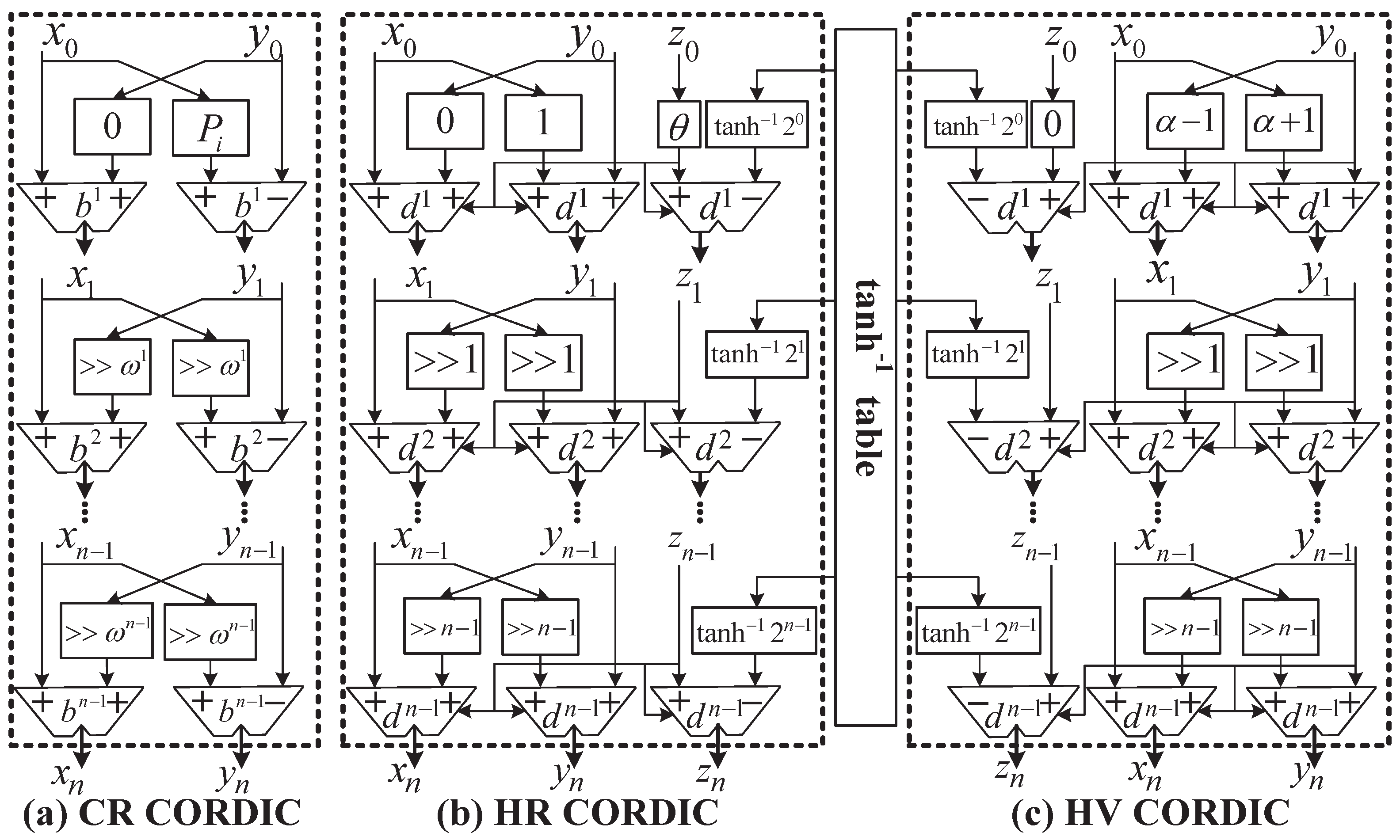
We design and implement a scalable hardware architecture to enhance flexibility and applicability. Based on the improved CORDIC algorithm, the convergence domains of e-exponent, logarithm, and square root functions are expanded to achieve temporally correlated fading in different scenarios. Furthermore, we adopt the SoFM method to ensure the continuity of the Doppler phase in non-stationary scenarios.

(2)

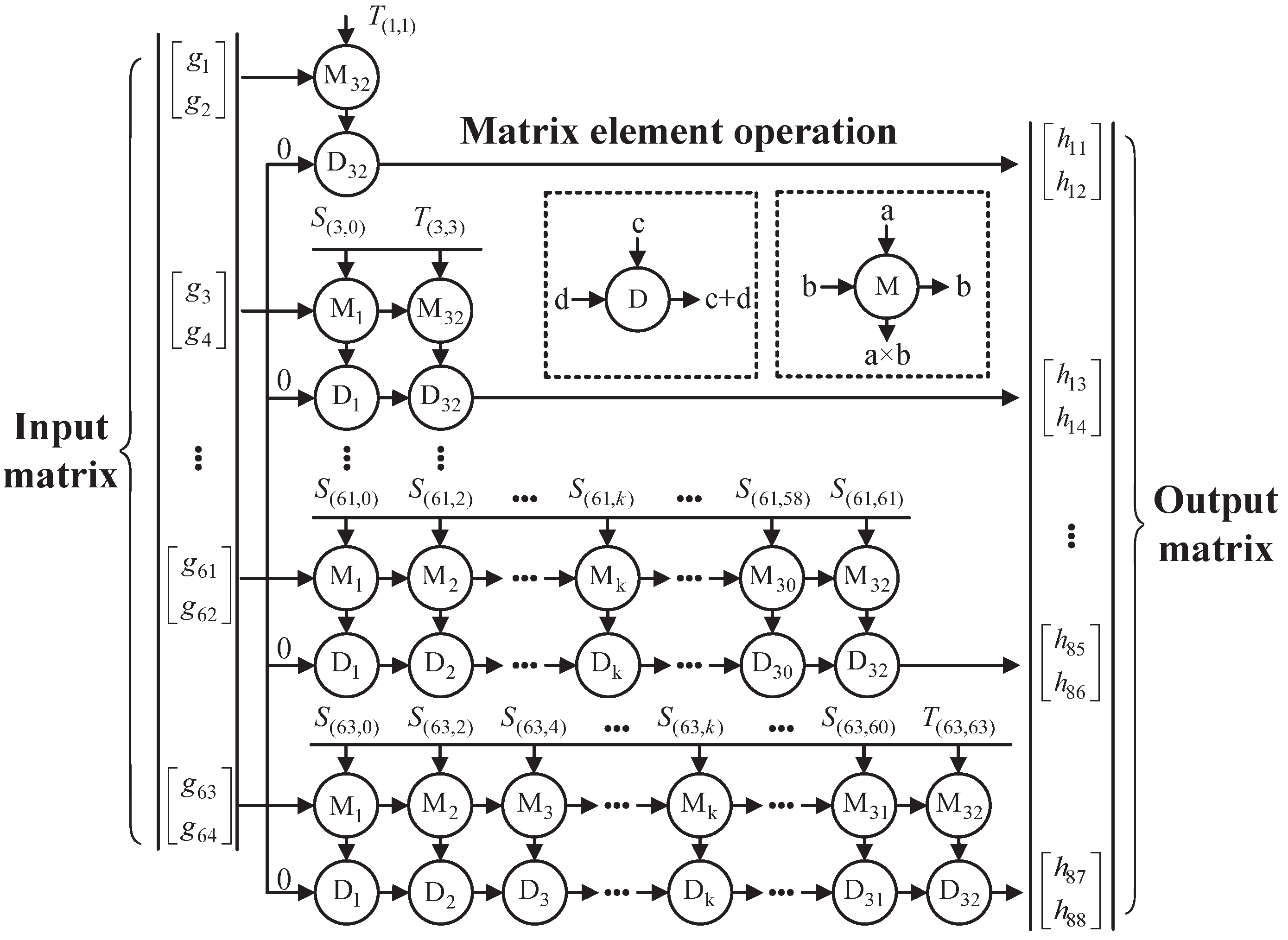
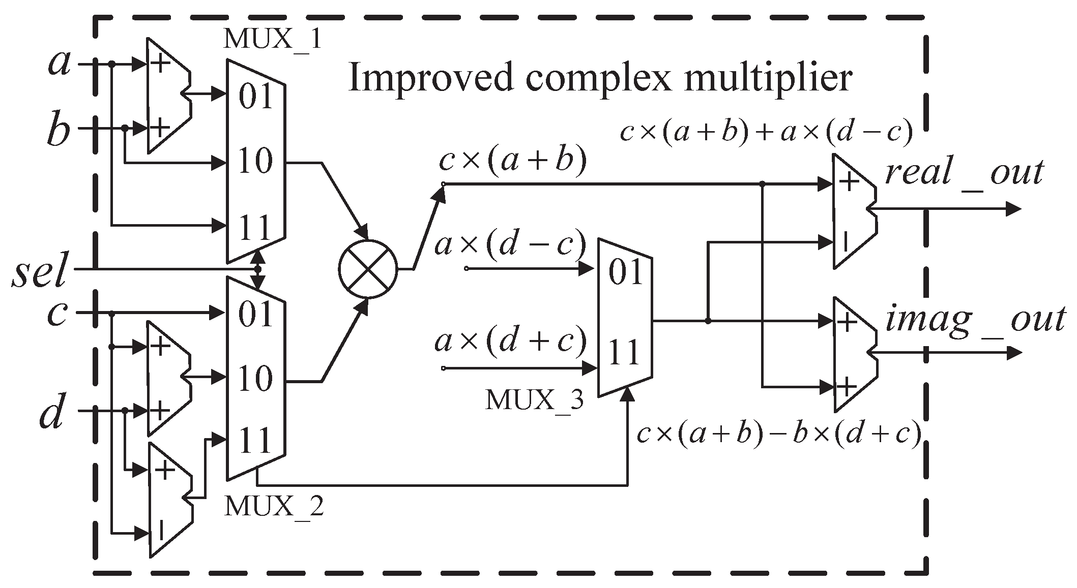
A lower triangular matrix operation method is proposed, which decomposes its large-scale matrix into low-level matrix operations. This is based on matrix partitioning and time-division multiplexing, which greatly reduces the complexity of hardware implementation for spatially correlated fading. In addition, a selector-based optimization scheme is adopted for complex multiplication, which effectively reduces hardware resource consumption.

(3)

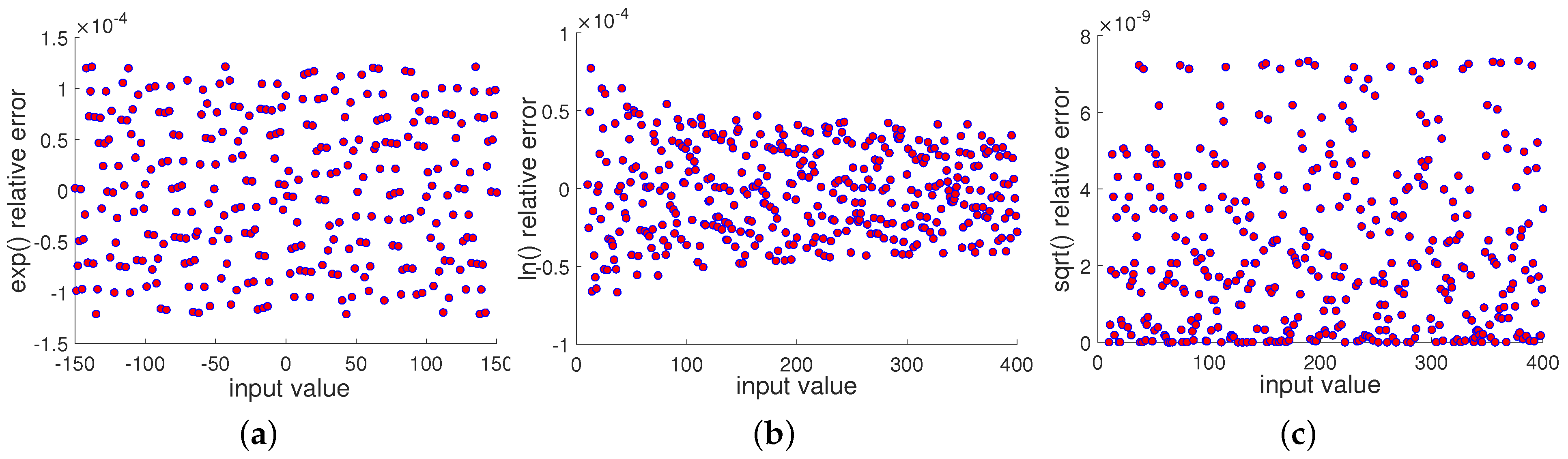
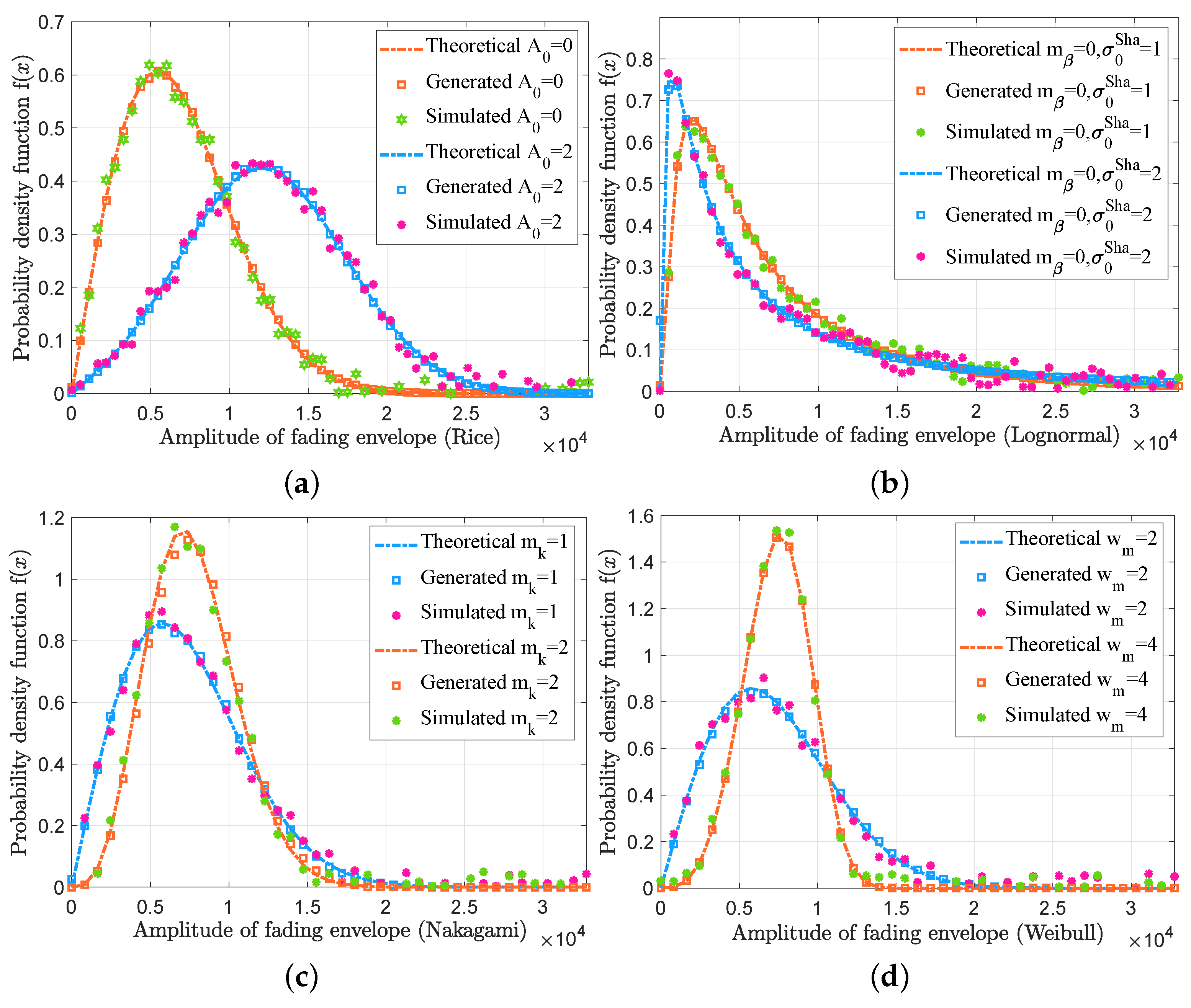
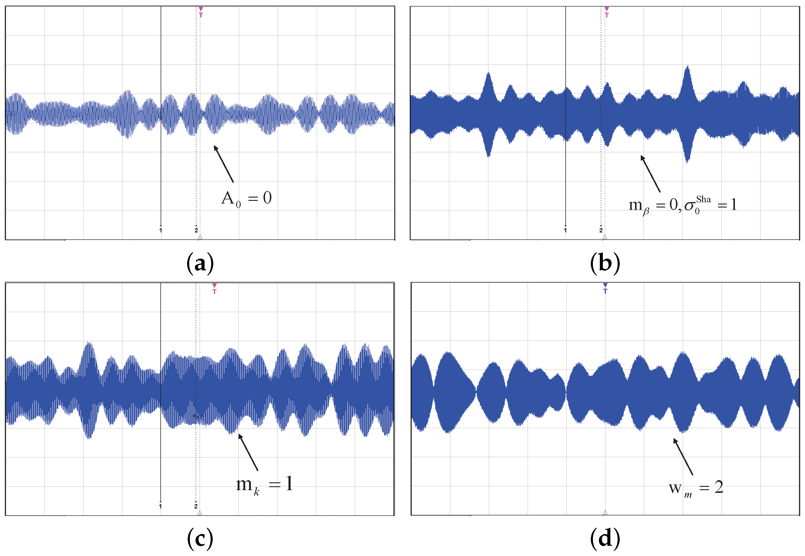
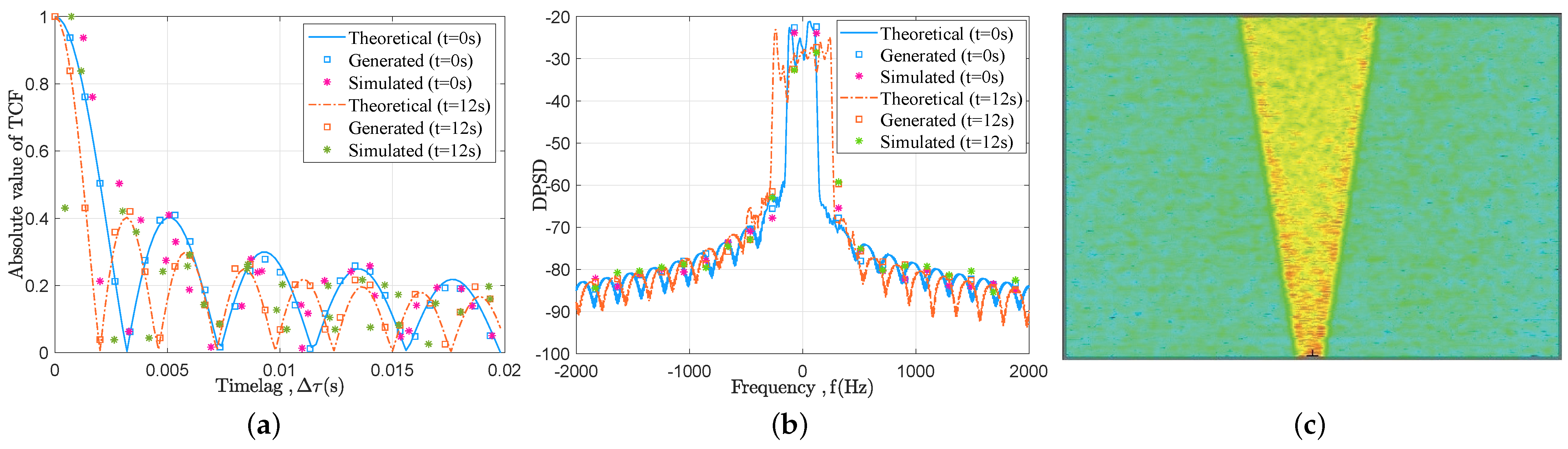
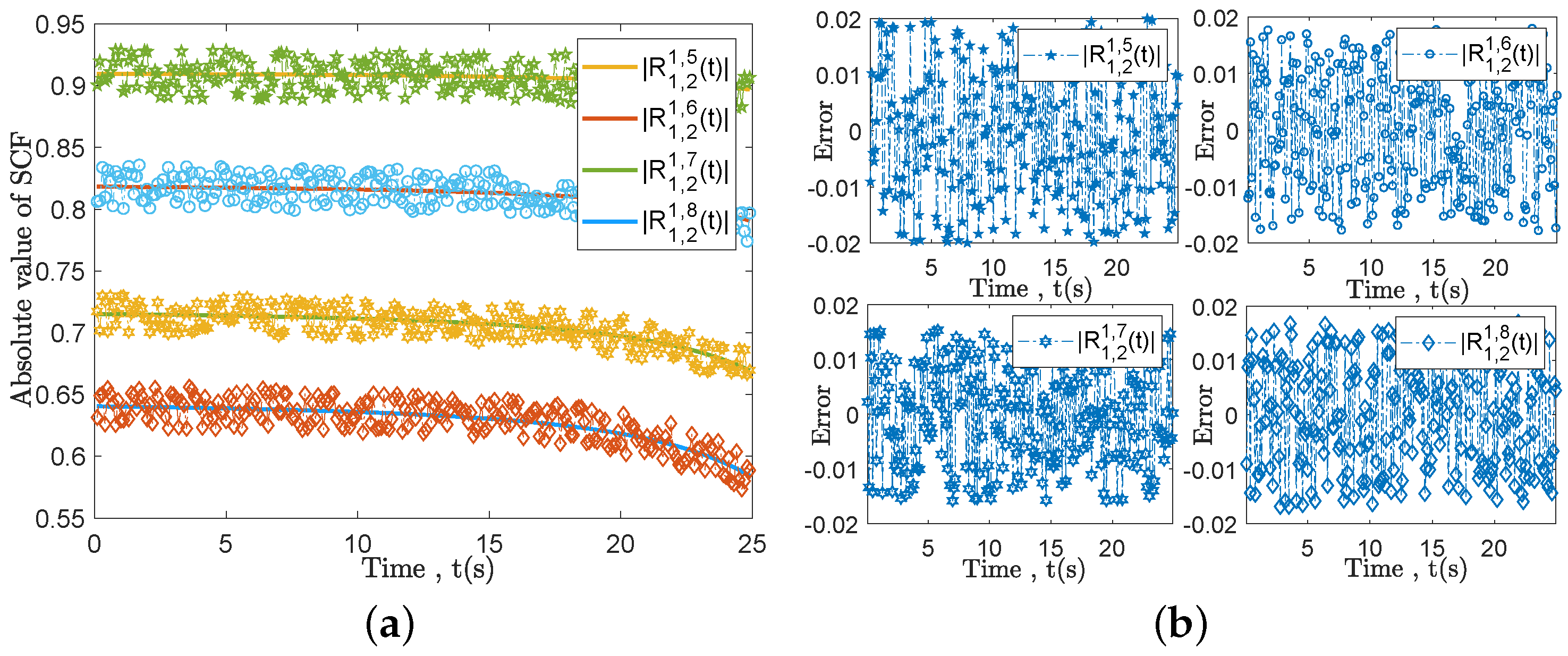
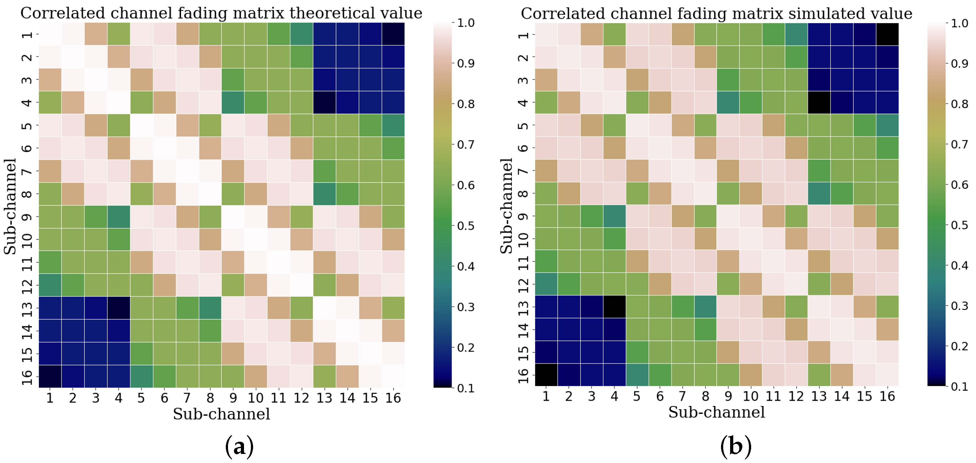
The proposed hardware generation method is implemented on the XC7VX690T FPGA chip. The hardware simulation results demonstrate that the statistical properties, such as the probability density function (PDF), Doppler power spectrum density (DPSD), temporal correlation function (TCF), and spatial correlation function (SCF), are in good agreement with their theoretical values. Specifically, the generated PDF error with a 16-bit fixed-point is 1.52%, and the average SCF error is 1.47%. In addition, resource utilization is reduced from 9.08% to 3.54%; DSP resources are especially reduced, with a reduction of 11.11%.

The remaining sections are organized as follows: Section 2 provides a brief overview of the theoretical generation method. Section 3 presents the FPGA hardware generation scheme and implementation details. In Section 4, the proposed method is implemented and verified on an FPGA platform. Finally, Section 5 presents the conclusions.

2. Correlated Channel Fading Model

Wireless signals propagate along various paths with different delays, powers, and angles. This causes unpredictable signal attenuation known as channel fading $p_n^i\left(t\right)$, which can be expressed as

$$p_n^i\left(t\right)=r_n^i\left(t\right)·exp\left\{j{\phi }_n^i\left(t\right)\right\},n=1,2,\cdots ,N$$

(1)

where $r_n^i\left(t\right)$ denotes the envelope of channel fading, $i\in \left\{\mathrm{Ray},\mathrm{Ric},\mathrm{Nak},\mathrm{Web},\mathrm{Sha}\right\}$, ${\phi }_n^i\left(t\right)$ denotes the random phase of channel fading and obeys the uniform distribution of $U\sim \left(0,2\pi \right]$, and $\mathit{N}$ denotes the number of multipath clusters. Different types of channel fading occur due to various channel propagation scenarios. In the non-line of sight (NLoS) propagation environment, the PDF of the Rayleigh fading envelope can be expressed as

$$f_r^{\mathrm{Ray}}\left(x\right)=\frac{x}{{\sigma }_0^2}exp(\frac{-x^2}{2{\sigma }_0^2})$$

(2)

where ${\sigma }_0$ is the standard deviation. In the line of sight (LoS) propagation environment, the PDF of the Rician fading envelope can be expressed as

$$f_r^{\mathrm{Ric}}\left(x\right)=\frac{x}{{{\sigma }_0}^2}·exp\left(\frac{x^2+A_0^2}{2{{\sigma }_0}^2}\right)·J_0(\frac{x{A}_0}{{{\sigma }_0}^2})$$

(3)

where $A_0$ represents the signal amplitude, and $J_0(·)$ represents the zero-order modified Bessel function of the first kind. The multipath fading due to the superposition of NLoS components can be modeled by the Nakagami distribution, and its envelope PDF can be expressed as

$$f_r^{\mathrm{Nak}}\left(x\right)=\frac{2}{\mathrm{\Gamma }\left(m_k\right)}{\left(\frac{m_k}{{\mathrm{\Omega }}_k}\right)}^{m_k}·x^{2m_k-1}·exp\left(-\frac{m_k}{{\mathrm{\Omega }}_k}{x}^2\right)$$

(4)

where $\mathrm{\Gamma }\left(m_k\right)$ denotes the gamma function, $m_k$ represents the shape factor which can evaluate the severity of channel fading, and ${\mathrm{\Omega }}_k$ represents the average power of each cluster. Furthermore, Weibull fading is more consistent with channel fading in indoor and outdoor environments. The PDF of the Weibull fading amplitude can be expressed as

$$f_r^{\mathrm{Web}}\left(x\right)=\frac{m_{\gamma }}{{\beta }_w}{\left(\frac{x}{{\beta }_w}\right)}^{m_{\gamma }-1}·exp{\left(\frac{x}{{\beta }_w}\right)}^{m_{\gamma }}$$

(5)

where $m_{\gamma }$ determines the shape of the magnitude PDF, and ${\beta }_w$ represents the scale parameter. In addition, the PDF of the shadow fading envelope can be further expressed as

$$f_r^{\mathrm{Sha}}\left(x\right)=\frac{1}{\sqrt{2\pi }{\sigma }_{0}x}exp\left[-\frac{{(lnx-m_{\beta })}^2}{2{{\sigma }_0}^2}\right]$$

(6)

where the measured data show that ${\sigma }_0\in \left[1.5,7\right]\mathrm{dB}$, and $m_{\beta }$ represents the mean value.

The TCF is a crucial tool in wireless channel modeling, providing information about the temporal characteristics of the channel. It helps estimate the coherence time and the severity of the channel fading. In a MIMO communication system, a single cluster signal will be affected by obstacles, and there is an autocorrelation characteristic between different time delays. It can be expressed as

$$A_n^{p^i}\left(\tau \right)=\frac{\mathrm{E}\left[p_n^i\left(t\right)p_n^i(t+\tau )\right]-\mathrm{E}\left[p_n^i\left(t\right)\right]\mathrm{E}\left[p_n^i(t+\tau )\right]}{\mathrm{var}\left[p_n^i(t+\tau )\right]}$$

(7)

where $\tau$ represents the time delay, $n\in \{1,2,\cdots ,N\}$, and $\mathrm{E}\left[·\right]$ and $var\left[·\right]$ denote the expectation and variance, respectively. If the scattering or reflection comes from the same scatterer or reflector, there will be a cross-correlation between the fading of each sub-channel in the communication system, its SCF can be expressed as

$$R_{k,l}^{p^i}\left(\tau \right)=\frac{\mathrm{E}\left[p_k^i\left(t\right)p_l^i(t+\tau )\right]-\mathrm{E}\left[p_k^i\left(t\right)\right]\mathrm{E}\left[p_l^i(t+\tau )\right]}{\sqrt{\mathrm{var}\left[p_k^i\left(t\right)\right]}·\sqrt{\mathrm{var}\left[p_l^i(t+\tau )\right]}}$$

(8)

where $\forall k\ne l$ and $k,l\in \left\{1,2,\cdots ,N\right\}$, $R_{k,l}^{p^i}$ represents the cross-correlation coefficient between the fading of the k-th channel and the i-th channel.

3. Scalable and Real-Time Hardware Generation Method

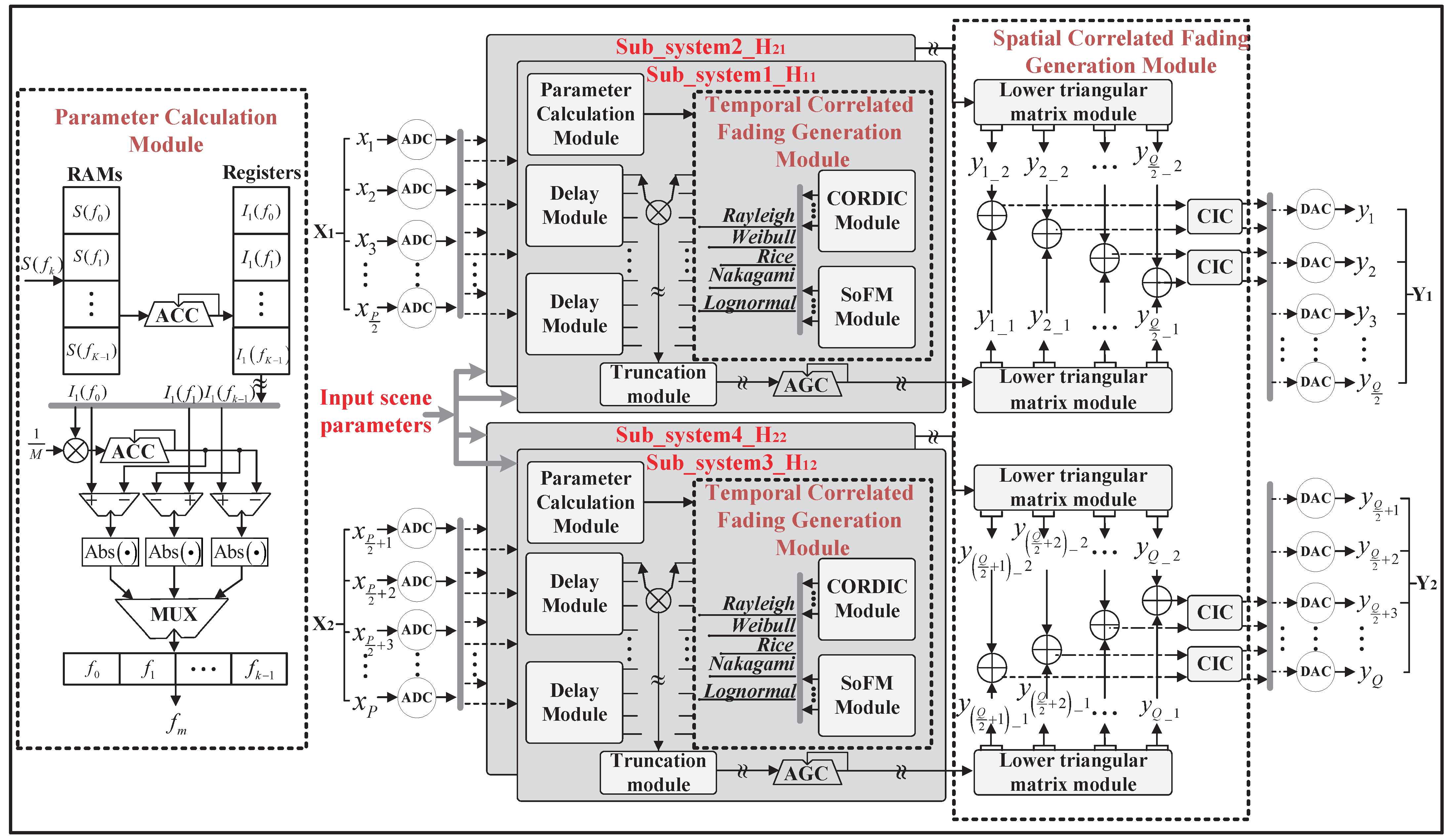
3.1. Overview of Hardware Generation Structure

For MIMO systems, traditional hardware implementation methods for channel simulation consist of pre-storage and real-time methods. The pre-storage generation algorithm requires a large amount of storage, and it is challenging to support time-varying dynamic scenes. On the other hand, the real-time generation algorithm involves a large amount of computation, and it is difficult to support large-scale multi-channel scenarios. Therefore, a flexible and real-time hardware generation architecture is established using the matrix block approach shown in Figure 1. The correlation sub-matrices ${\mathbf{H}}_{11}$, ${\mathbf{H}}_{12}$, ${\mathbf{H}}_{21}$, and ${\mathbf{H}}_{22}$ are expressed as:

$$\begin{array}{c}{\mathbf{H}}_{\left(i+1\right)\left(j+1\right)}=\left[\begin{array}{cccc}{h}_{\left(\frac{P}{2}·i+1\right)\left(\frac{Q}{2}·j+1\right)}& h_{\left(\frac{P}{2}·i+1\right)\left(\frac{Q}{2}·j+2\right)}& \cdots & h_{\left(\frac{P}{2}·i+1\right)\left(\frac{Q}{2}·j+\frac{Q}{2}\right)}\\ h_{\left(\frac{P}{2}·i+2\right)\left(\frac{Q}{2}·j+1\right)}& h_{\left(\frac{P}{2}·i+2\right)\left(\frac{Q}{2}·j+2\right)}& \cdots & h_{\left(\frac{P}{2}·i+2\right)\left(\frac{Q}{2}·j+\frac{Q}{2}\right)}\\ ⋮& ⋮& \ddots & ⋮\\ h_{{}_{\left(\frac{P}{2}·i+\frac{P}{2}\right)\left(\frac{Q}{2}·j+1\right)}}& h_{\left(\frac{P}{2}·i+\frac{P}{2}\right)\left(\frac{Q}{2}·j+2\right)}& \cdots & h_{\left(\frac{P}{2}·i+\frac{P}{2}\right)\left(\frac{Q}{2}·j+\frac{Q}{2}\right)}\end{array}\right]\end{array}$$

(9)

where $i,j\in \left\{0,1\right\}$, $h_{qp}$ represents the sub-channel fading, and P and Q denote the number of transmitting antennas and the number of receiving antennas, respectively.

It can be seen from the figure that ${\mathbf{X}}_1$ and ${\mathbf{X}}_2$ are channel transmission sub-matrices, and ${\mathbf{Y}}_1$ and ${\mathbf{Y}}_2$ are channel receiving sub-matrices, which can be expressed as

$${\mathbf{X}}_1={\left[\begin{array}{cccc}{x}_1& x_2& \cdots & x_{\frac{P}{2}}\end{array}\right]}^T,{\mathbf{X}}_2={\left[\begin{array}{cccc}{x}_{\left(\frac{P}{2}+1\right)}& x_{\left(\frac{P}{2}+2\right)}& \cdots & x_P\end{array}\right]}^T$$

(10)

$${\mathbf{Y}}_1={\left[\begin{array}{cccc}{y}_1& y_2& \cdots & y_{\frac{Q}{2}}\end{array}\right]}^T,{\mathbf{Y}}_2={\left[\begin{array}{cccc}{y}_{\left(\frac{Q}{2}+1\right)}& y_{\left(\frac{Q}{2}+2\right)}& \cdots & y_Q\end{array}\right]}^T$$

(11)

In (10), $x_p$ denotes the signal transmitted by the p-th antenna. In (11), $y_q$ denotes the signal received by the q-th antenna, which can be expressed as

$$y_q=y_{q\_1}+y_{q\_2}=(y_{q1}+y_{q2}+\cdots +y_{q\frac{P}{2}})+(y_{q\left(\frac{P}{2}+1\right)}+y_{q\left(\frac{P}{2}+2\right)}+\cdots +y_{qP})$$

(12)

where $y_{q\_1}$ and $y_{q\_2}$ denote the channel components output by the superposition of the two subsystems after the matrix block in the MIMO system, and $y_q$ denotes the output of their superposition. In (12), $y_{qp}=h_{qp}·x_p(q=2,\cdots ,Q,p=2,\cdots ,P)$ and $h_{qp}$ can be obtained by the generation method of spatial–temporal correlated channel fading. We divide the simulation unit into four subsystems with the same structure for parallel computing, which reduces system complexity, increases maintainability, and has better real-time performance. The above single-cluster correlated fading can be obtained by applying a series of nonlinear transformations to the Gaussian sequence. In practice, the channel fading in most scenarios presents non-stationary characteristics. The SoFM method is used to generate the Gaussian random variable ${\widehat{\sigma }}_n\left(\xi \right)$, which can be expressed as

$${\widehat{\sigma }}_n\left(\xi \right)=\frac{1}{\sqrt{M}}\sum _{m=1}^{M}exp\left\{j(2\pi \sum _{k=0}^{\xi }{T}_s{\widehat{f}}_{n,m}\left[k\right]+{\widehat{\phi }}_{n,m})\right\}=\frac{1}{\sqrt{M}}\sum _{m=1}^{M}exp\left\{j\left({\widehat{\theta }}_{n,m}\left(\xi \right)\right)\right\}$$

(13)

where $\xi$ represents the time index of the discrete domain, $\mathit{M}$ denotes the number of frequency modulation, $T_s$ represents the clock period of hardware, and ${\widehat{\theta }}_{n,m}$, ${\widehat{f}}_{n,m}$, and ${\widehat{\phi }}_{n,m}$ denote the time-varying phase, discrete Doppler frequency, and initial phase, respectively. The initial phase is uniformly distributed over $\left(0,2\pi \right]$.

The discrete Doppler frequency ${\widehat{f}}_{n,m}$ can be characterized by the DPSD ${\widehat{S}}_{{\sigma }_n{\sigma }_n}\left(f\right)$. We first divide the DPSD into $\mathit{M}$ parts and determine ${\widehat{f}}_{n,m}$ with the MEA method [24], which can be expressed as

$${\int }_{f_{m-1}}^{f_m}{\widehat{S}}_{{\sigma }_n{\sigma }_n}\left(f\right)df=\sum _{f_k=f_{m-1}}^{f_m}{\widehat{S}}_{{\sigma }_n{\sigma }_n}\left(f_k\right)·\frac{2f_m^{max}}{K}=\frac{{\nu }_n^2}{M}$$

(14)

where ${\nu }_n^2$ denotes the average power of channel fading, $f_m$ represents the m-th discrete Doppler frequency, and $f_m^{max}$ and $\mathit{K}$ denote the maximum Doppler frequency and the number of frequency domain sampling points for DPSD, respectively. We introduce the auxiliary function ${\widehat{I}}_{n,m}\left(f_k\right)$, which can be expressed as

$${\widehat{I}}_{n,m}\left(f_k\right)=\sum _{f_k=f_0}^{f_k}{\widehat{S}}_{{\sigma }_n{\sigma }_n}\left(f_k\right)-\frac{m}{M}·\sum _{f_k=f_0}^{f_{k-1}}{\widehat{S}}_{{\sigma }_n{\sigma }_n}\left(f_k\right)$$

(15)

where $f_0$ denotes the spectrum offset, and $f_k$ represents the discrete frequency stepping. Assuming that the inverse function ${{\widehat{I}}_{n,m}}^{-1}\left(f_k\right)$ exists, the discrete Doppler frequency ${\widehat{f}}_{n,m}$ can be further expressed as ${\widehat{f}}_{n,m}={{\widehat{I}}_{n,m}}^{-1}\left(0\right)$. Rayleigh fading can be expressed as the complex sum of two sets of mutually orthogonal Gaussian random sequences

$${\widehat{r}}_n^{\mathrm{Ray}}\left(\xi \right)=\left|{\widehat{\sigma }}_{n,1}\left(\xi \right)+j{\widehat{\sigma }}_{n,2}\left(\xi \right)\right|$$

(16)

where ${\sigma }_{n,1}\left(\xi \right)$ and ${\sigma }_{n,2}\left(\xi \right)$ represent the in-phase component and the quadrature component of the Gaussian random sequence, respectively. Rice fading can be simulated by superimposing the line-of-sight path on the basis of Rayleigh fading, which can be expressed as

$${\widehat{r}}_n^{\mathrm{Ric}}\left(\xi \right)=\left|{\rho }_m·exp\left(j(\sum _{k=0}^{\xi }{T}_s{\widehat{f}}_{LoS}\left[k\right]+{\widehat{\phi }}_{LoS})\right)+{\widehat{r}}_n^{\mathrm{Ray}}\left(\xi \right)\right|$$

(17)

where ${\rho }_m$ represents the amplitude, ${\widehat{f}}_{LoS}$ and ${\widehat{\phi }}_{LoS}$ denote the Doppler frequency and initial phase of LoS component, respectively. The Formula (17) can be transformed into Rayleigh fading When ${\rho }_m=0$. Nakagami fading can be simulated by several independent Gaussian random sequences, which can be further expressed as

$$\begin{array}{c}{\widehat{r}}_n^{\mathrm{Nak}}\left(\xi \right)=\sqrt{{{\zeta }_n}^{Sha}/2m}·\sqrt{{\left[{\widehat{\sigma }}_{n,1}\left(\xi \right)\right]}^2+{\left[{\widehat{\sigma }}_{n,2}\left(\xi \right)\right]}^2+\cdots +{\left[{\widehat{\sigma }}_{n,2m}\left(\xi \right)\right]}^2}\hfill \end{array}$$

(18)

where ${{\zeta }_n}^{Sha}$ represents the average power of each cluster signal fading. According to the measured data, Weibull fading can be generated by two Gaussian random sequences with zero mean and orthogonal to each other, which can be further expressed as

$$\begin{array}{c}{\widehat{r}}_n^{\mathrm{Web}}\left(\xi \right)=exp(w_m/\phantom{w_{m}2}2·ln\left({\widehat{\sigma }}_{n,1}\left(\xi \right)+j{\widehat{\sigma }}_{n,2}\left(\xi \right)\right)=exp\left(w_m/\phantom{w_{m}2·ln\left({\widehat{r}}_n^{\mathrm{Ray}}\left(\xi \right)\right)}2·ln\left({\widehat{r}}_n^{\mathrm{Ray}}\left(\xi \right)\right)\right)\end{array}$$

(19)

where $w_m$ represents Weibull form factor, when $w_m=2$, (19) degenerates to a Rayleigh distribution. Furthermore, shadow fading can usually be modeled as a Lognormal distribution, which can be further expressed as

$${{\widehat{r}}_n}^{\mathrm{Sha}}\left(\xi \right)=exp\left({\xi }_{n,\beta }{\widehat{\sigma }}_{n,0}\left(\xi \right)+{\alpha }_{n,\beta }\right)$$

(20)

where ${\xi }_{n,\beta }$ and ${\alpha }_{n,\beta }$ denote the standard deviation and mean of shadow fading, respectively. Based on the above, the types of channel fading that can be implemented by this hardware architecture are summarized in

Table 1. The fading types supported by the hardware architecture.

Fading Type	Fading Symbol	Communication Scenario
Rayleigh	${\widehat{r}}_n^{\mathrm{Ray}}\left(\xi \right)$	Urban high-rise environments without LoS
Rice	${\widehat{r}}_n^{\mathrm{Ric}}\left(\xi \right)$	Urban and suburban areas with LoS
Nakagami	${\widehat{r}}_n^{\mathrm{Nak}}\left(\xi \right)$	High-rise buildings and rural areas
Weibull	${\widehat{r}}_n^{\mathrm{Web}}\left(\xi \right)$	Urban areas
Shadow	${\widehat{r}}_n^{\mathrm{Sha}}\left(\xi \right)$	Tall buildings and terrain obstacles

.

3.2. Temporal Correlated Fading Generation Based on Modified CORDIC Method

In various communication scenarios, real-time calculations of the complex exponential, e-exponent, natural logarithm, and square root functions are required for generating channel fading. To date, the above functions can be implemented through the LUT and CORIDC methods. However, the classical CORDIC method has too many iterations, poor real-time performance, and limited input convergence domain, making it unsuitable for the real-time operation of numerous fixed-point data. Figure 2 depicts the hardware implementation architecture of the CORDIC algorithm, where the above function values can be computed using rotation and vector modes in different coordinate systems.

In the rotation mode of the circular system, using the improved CORDIC method can reduce the hardware delay and consumption of the real-time operation of the complex exponential, as shown in Figure 2a. For a hyperbolic coordinate system, the target angle $\theta$ can be defined as a set of angles $\{1\le i\le L-1|{\theta }^i={tanh}^{-1}\left(2^{-i}\right)\}$ that satisfy the approximate relation $tan{\theta }^i\approx 2^{-i}$, where L denotes the fixed-point data bit width length, and i denotes the number of current iterations. As shown in Figure 2b, the iterative process of calculating the value of the hyperbolic sine–cosine function can be expressed as

$$\left[\begin{array}{c}{x}_{i+1}^{HR}\\ y_{i+1}^{HR}\\ z_{i+1}^{HR}\end{array}\right]=\left[\begin{array}{ccc}1& d_i^{HR}·2^{-i}& 0\\ d_i^{HR}·2^{-i}& 1& 0\\ 0& 0& 1\end{array}\right]\left[\begin{array}{c}{x}_i^{HR}\\ y_i^{HR}\\ z_i^{HR}\end{array}\right]+\left[\begin{array}{c}0\\ 0\\ -d_i^{HR}·{tanh}^{-1}{2}^{-i}\end{array}\right]$$

(21)

$$d_i^{HR}=\left\{\begin{array}{c}+1,z_i^{HR}\ge 0\\ -1,z_i^{HR}<0\end{array}\right.$$

(22)

where $z_i^{HR}$ denotes the remaining rotation angle, $d_i^{HR}=\pm 1$ represents the rotation direction factor, and i denotes the number of current iterations. For the iterative process of the hyperbolic system, when the iteration number satisfies $i=3k+1$, the iteration must be repeated. In CORDIC hyperbolic coordinate rotation mode, the final output value can be expressed as

$$\begin{array}{c}{x}_n^{HR}=A_n^{HR}(x_1^{HR}cosh{z}_1^{HR}+y_1^{HR}sinh{z}_1^{HR})\hfill \\ y_n^{HR}=A_n^{HR}(x_1^{HR}sinh{z}_1^{HR}+y_1^{HR}cosh{z}_1^{HR})\hfill \\ z_n^{HR}=0\hfill \end{array}$$

(23)

where $A_n^{HR}={\prod }_{i=1}^{n-1}\sqrt{1-2^{-2i}}$ when $n\to \infty$,$A_n^{HR}\approx 0.82815936$; therefore, the modulo length compensation factor is $K_n^{HR}\approx 1.20749706$. The sum of the rotation angles is ${\sum }_{i=1}^{\infty }{tanh}^{-1}{2}^{-i}=1.1181$, and the value $z_i^{HR}$ range of the input angle is limited to $\left[-1.1181,+1.1181\right]$. Set the initial value $x_1^{HR}=1,y_1^{HR}=0,z_1^{HR}=\theta$; then, Equation (23) can be further expressed as

$$\begin{array}{c}{x}_n^{HR}=cosh\theta /K_n^{HR}\hfill \\ y_n^{HR}=sinh\theta /K_n^{HR}\hfill \\ z_n^{HR}=0\hfill \end{array}$$

(24)

However, in the nonlinear function transformation based on Gaussian sequence, taking lognormal fading as an example, the actual input angle will be outside the convergence region, so it is necessary to expand the convergence region. We can convert the input angle $z_1^{HR}=\theta$ into the form of $z_1^{HR}=Q·ln2+R$, where $\mathit{Q}$ is the rounded value of $\theta /ln2$, and R is the value of the remainder of $\theta /ln2$.

The corresponding exponential output can be converted to the form of $e^{z_1^{HR}}=2^Q·e^R$, and the extent of the input angle convergence region increases with the value of $\mathit{Q}$. Figure 3a shows the relative error of the e-exponential function calculation after expanding the range of convergence region. It can be seen from the figure that when the range of the extended convergence domain is $[-150,150]$, the relative error range of the e-exponential function calculation is maintained within the order of $[-1.21,+1.21]\times {10}^{-4}$, which meets the data accuracy requirements of the hardware system.

As shown in Figure 2c, the hyperbolic coordinate rotation vector mode in CORDIC is used to calculate the logarithmic function and square root function. Different from the rotation mode, the rotation factor $d_i^{HV}$ in (21) is determined by $y_i^{HV}$,

$$d_i^{HV}=\left\{\begin{array}{c}+1,y_i^{HV}\le 0\\ -1,y_i^{HV}>0\end{array}\right.$$

(25)

the last iteration output value in vector mode can be expressed as

$$\begin{array}{c}{x}_n^{HV}=A_n^{HV}\sqrt{{x_1^{HV}}^2-{y_1^{HV}}^2}\hfill \\ y_n^{HV}=0\hfill \\ z_n^{HV}=z_1^{HV}+{tanh}^{-1}(y_1^{HV}/x_1^{HV})\hfill \end{array}$$

(26)

Set the initial value $x_1^{HV}=\theta +1, y_1^{HV}=\theta -1, z_1^{HV}=0$; then, Equation (26) can be further expressed as

$$\begin{array}{c}{x}_n^{HV}=2A_n^{HV}\sqrt{\theta }\hfill \\ y_n^{HV}=0\hfill \\ z_n^{HV}={tanh}^{-1}\left(\theta -1/\theta +1\right)\hfill \end{array}$$

(27)

With $ln\theta =2·ta{n}^{-1}h\left(\theta -1/\theta +1\right)$, we obtain $z_n^{HV}=ln\theta /2$. To extend the domain of convergence, we can convert the input angle $z_1^{HV}=\theta$ into the form $\theta =\alpha ·4^Q$, and the corresponding logarithmic function output becomes $ln\theta =ln\alpha +Q·2ln2$, where $\alpha \in [0.1069,9.3573]$, and $\mathit{Q}$ is an integer. The range of input $\theta$ is related to the value range of $\mathit{Q}$. If the convergence area continues to expand, we need to change the value range of $\mathit{Q}$.

For hardware implementation, $2^Q$ can be implemented by shifting, which facilitates a fixed point of the input angle. Figure 3b,c shows the relative error calculated by the logarithmic function and the square root function after expanding the range of convergence. It can be seen from the figure that when the range of the extended convergence domain is $[10,400]$, the relative error range of the logarithmic function is within the order of $[-6.66,+7.72]\times {10}^{-5}$ and the relative error range of the square root function is within the order of $[+0.01,+7.23]\times {10}^{-9}$, both of which meet the requirements of the hardware system for data accuracy.

3.3. Spatial Correlated Fading Generation Based on Efficient Matrix Operation

The complex Gaussian fading channel matrix ${\widehat{\mathbf{G}}}_{u,s}\left(t\right)$ can be obtained through the temporal correlated fading generation module, and each element is independent of each other. Based on (8), the correlation channel fading coefficient matrix ${\widehat{\mathbf{R}}}_{u,s}\left(t\right)$ can be further generated; then, the channel correlation matrix ${\widehat{\mathbf{H}}}_{u,s}\left(t\right)$ can be expressed as

$$vec\left[{\widehat{\mathbf{H}}}_{u,s}\left(t\right)\right]={\widehat{\mathbf{R}}}_{u,s}{\left(t\right)}^{1/2}·vec\left[{\widehat{\mathbf{G}}}_{u,s}\left(t\right)\right]$$

(28)

where $u,s=1,2,\dots ,N$, and $\mathrm{vec}[·]$ represents the vector operator. The lower triangular coefficient matrix ${\widehat{L}}_{u,s}\left(t\right)$ can be obtained by decomposing ${\widehat{\mathbf{R}}}_{u,s}\left(t\right)$ using the Cholesky decomposition, and it satisfies ${\widehat{L}}_{u,s}\left(t\right)={\widehat{\mathbf{R}}}_{u,s}{\left(t\right)}^{1/2}$. It is essential to develop a lower triangular matrix calculation algorithm to reduce resource consumption, taking the 8x8 MIMO system as an example, the correlation matrix ${\widehat{L}}_{8,8}$ can be expressed as

$${\widehat{L}}_{8,8}=\left[\begin{array}{cccc}{l}_{(1,1)}& & & \\ l_{(2,1)}& l_{(2,2)}& & \\ ⋮& ⋮& \ddots & \\ l_{(64,1)}& l_{(64,2)}& \cdots & l_{(64,64)}\end{array}\right]$$

(29)

where $l_{(i,j)}$ denotes the correlation coefficient between sub-channels. The complex Gaussian fading matrix ${\widehat{G}}_{8,8}$ is represented in vector form as

$$\mathrm{vec}\left[{\widehat{\mathbf{G}}}_{8,8}\right]={\left[\begin{array}{cccc}{g}_1& g_2& \cdots & g_{64}\end{array}\right]}^T$$

(30)

where $g_i$ denotes the independent sub-channel fading. In (29), ${\widehat{L}}_{8,8}$ is a lower triangular matrix of order 64; it obtains the smallest constituent element of the block matrix in (9) by multiplying and accumulating with $\mathrm{vec}\left[{\widehat{\mathbf{G}}}_{8,8}\right]$. Due to the high hardware resource consumption and computational complexity involved in the matrix operation process, it is not conducive to hardware implementation and maintenance. To overcome these challenges, a matrix block approach can be used to partition the lower triangular matrix into smaller blocks. Here, the $64\times 64$ correlation matrix ${\widehat{L}}_{8,8}$ is divided into a second-order matrices, $S_{(m,n)}$ and $T_{(i,i)}$. This approach simplifies the complex matrix operations into minimal units, thereby reducing the complexity of hardware implementation. Specifically, $S_{(m,n)}$ and $T_{(i,i)}$ can be expressed as

$$\begin{array}{c}{T}_{(i,i)}=\left[\begin{array}{cc}{l}_{(i,i)}& \\ l_{(i+1,i)}& l_{(i+1,i+1)}\end{array}\right],S_{(m,n)}=\left[\begin{array}{cc}{l}_{(m,n+1)}& l_{(m,n+2)}\\ l_{(m+1,n+3)}& l_{(m+1,n+4)}\end{array}\right]\end{array}$$

(31)

In (31), the variable $i,m,n$ interval is 2, where $i=1,3,5,\cdots ,63$, $m=3,5,\cdots ,63$ and $n=0,2,\cdots ,m-3$. Finally, the large-scale lower triangular matrix ${\widehat{L}}_{8,8}$ can be decomposed into 32 second-order lower triangular matrix $T_{(i,i)}$ and 496 second-order square matrices $S_{(m,n)}$. From Equations (29) and (31), the lower triangular matrix ${\widehat{L}}_{8,8}$ can be expressed as

$${\widehat{L}}_{8,8}=\left[\begin{array}{cccc}{T}_{(1,1)}& & & \\ S_{(3,0)}& T_{(3,3)}& & \\ ⋮& ⋮& \ddots & \\ S_{(63,0)}& S_{(63,2)}& \begin{array}{cc}\cdots & S_{(63,60)}\end{array}& T_{(63,63)}\end{array}\right]$$

(32)

decompose $\mathrm{vec}\left[{\widehat{\mathbf{G}}}_{8,8}\right]$ into 32 second-order vectors as follows,

$$\mathrm{vec}\left[{\widehat{\mathbf{G}}}_{8,8}\right]={\left[\begin{array}{cccc}{\left(\begin{array}{cc}{g}_1& g_2\end{array}\right)}_1& {\left(\begin{array}{cc}{g}_3& g_4\end{array}\right)}_2& \cdots & {\left(\begin{array}{cc}{g}_{2i-1}& g_{2i}\end{array}\right)}_i\end{array}\right]}^T$$

(33)

where $i=1,2,\dots ,32$ and ${\left(·\right)}_i$ denotes a group of second-order vectors, $T_{(i,i)}$ and $S_{(m,n)}$ are the minimum constituent units of ${\widehat{L}}_{8,8}$, ${\left(\begin{array}{cc}{g}_{2i-1}& g_{2i}\end{array}\right)}_i$ is the minimum constituent units of $\mathrm{vec}\left[{\widehat{\mathbf{G}}}_{8,8}\right]$. If matrix operations are performed on all the minimum constituent units separately, a lot of multiplication resources will be consumed. To tackle this issue, a time-division multiplexing (TDM)-based method for lower triangular matrix multiplication is developed, which can further reduce hardware consumption. The scheme of the proposed method is given in Figure 4, the lower triangular matrix ${\widehat{L}}_{8,8}$ and the vector $\mathrm{vec}\left[{\widehat{\mathbf{G}}}_{8,8}\right]$ are multiplied by the time-division multiplexing architecture, and 32 second-order lower triangular matrix-vector multiplications and 496 second-order square matrix-vector multiplications can be converted into 1 second-order lower triangular matrix-vector multiplication and 31 second-order square matrix -vector multiplications, which can greatly reduce resource consumption.

As shown in the figure, $\mathrm{vec}\left[{\widehat{\mathbf{G}}}_{8,8}\right]$ as the input matrix, it is multiplied and accumulated by the lower triangular matrix ${\widehat{L}}_{8,8}$ in a time-division-multiplexed architecture, and the result $\mathrm{vec}\left[{\widehat{H}}_{8,8}\left(t\right)\right]$ is obtained as the output matrix. For complex multiplication operations, the consumption of multiplier resources can be further reduced by optimizing the hardware structure, as follows

$$\begin{array}{c}(a+bj)·(c+dj)=(ac-bd)+(bc+ad)j\\ =\left[c(a+b)-b(d+c)\right]+\left[c(a+b)+a(d-c)\right]j\end{array}$$

(34)

As shown in Figure 5, we implement complex multiplication based on the hardware architecture of the data selectors. From Equation (34), it can be known that the traditional complex multiplication architecture requires four multipliers and two adders or subtractors, and the other method requires three multipliers and five adders or subtractors, both of which consume more real multiplier logic resources. In Figure 5, the improved method optimizes the complex multiplication structure, improves the utilization efficiency, reduces the occupied area, and further reduces the hardware circuit cost.

It can be seen from the figure that $\mathit{sel}$ is used as a selection signal to control MUX_1 to output $\mathit{a}+\mathit{b}$, $\mathit{b}$, and $\mathit{a}$; control MUX_2 to output $\mathit{c}$, $\mathit{d}+\mathit{c}$, and $\mathit{d}-\mathit{c}$; and control MUX_3 to output $b\times (d+c)$ and $a\times (d-c)$. The improved complex multiplier structure uses only one multiplier unit, making it work in every clock cycle, which can greatly reduce the multiplier resources, save the occupied area, and reduce the hardware cost.

4. Measurement Results and Analysis

4.1. Statistical Properties of Generated Fading

To validate the proposed method in this paper, a $4\times 4$ MIMO channel fading emulation is implemented on a Xilinx XC7VX690T FPGA chip using the method proposed in this paper. Channel parameters such as carrier frequency, number of transmitting antennae, number of receiving antennae, delay, power, fading type, maximum Doppler frequency, subchannel correlation coefficients, emulation time, status update interval, and others are input into the FPGA platform using the VIVADO2020.2 software to generate output fading with specific channel characteristics. Additionally, the ILA tool in the VIVADO platform is utilized to capture the output data into MATLAB for the analysis of statistical characteristics of the output fading. Furthermore, the output fading envelope is observed using the Rohde & Schwarz RTM1054 oscilloscope, and the DPSD of the output fading is observed using the Agilent N9340B spectrum analyzer.

In order to verify the correctness of the method proposed in this paper in the generation of different output fading envelope distributions, the general scene parameters are set. Specifically, the number of transmitting antennae, the number of receiving antennae, the maximum Doppler frequency and data width are $P=1$, $Q=1$, $f_m^{max}=50\mathrm{Hz}$, and 16 bit, respectively. The fading type $\mathit{i}$ as is set as Rice, lognormal, Nakagami, or Weibull, and the emulation time of each fading is $t=15\mathrm{ms}$. The parameters are sent to the FPGA, and the data are captured by the ILA of the VIVADO platform and fed back to MATLAB for analysis. By using (3)–(6), Figure 6 shows the theoretical value, generated value, and hardware simulation value of the PDF of the time-varying correlation fading in the above scenario. It can be seen from the figure that the theoretical value is in good agreement with the generated value and the simulated value, and the average absolute deviation is about 1.52% and 2.47%, respectively.

Based on the above scenarios, we set ${\mathrm{A}}_0=0$, ${\mathrm{m}}_{\beta }=0,{\sigma }_0^{\mathrm{Sha}}=1$, ${\mathrm{m}}_k=1$, and ${\mathrm{w}}_m=2$, and use the RTM1054 oscilloscope from Rohde & Schwarz, to observe the waveforms of the relative fading envelopes in different scenarios, as shown in Figure 7. Taking Rice fading as an example, according to the actual simulation results, its fading shape meets the theoretical requirements.

In addition, to verify the reliability of the spatial–temporal correlation characteristics of channel fading, we set the carrier frequency, the number of transmitting antenna, the number of receiving antenna, the fading type, the emulation time, and the status update interval to $f_c=2.4\mathrm{GHz}$, $P=4$, $Q=4$, $i=\mathrm{Ric}$, $t=25\mathrm{s}$, and $t_0=20\mathrm{ms}$. In Figure 8a, the values of the theoretical time-varying TCF and the generated TCF, simulated TCF at t = 0 s and 12 s are compared in this simulation scenario. As shown in Figure 8a, the simulated TCF is in good agreement with the theoretical value, and the normalized TCF varies with time and has time-varying properties. Through the Fourier transform of TCF, one can further compute DPSD, and the measured results are shown in Figure 8c. For the sake of comparison, the DPSDs at the time points of t = 0 s and t = 12 s were extracted from Figure 8c, whereas their corresponding simulated counterparts are displayed in Figure 8b. The temporal evolution of DPSDs can be observed, exhibiting time-varying characteristics.

Based on the parameter setting of the above scene, the normalized omnidirectional antenna is used at the transceiver end, and the distance between the array elements is $0.5\lambda$. Figure 9a shows the comparison between the theoretical modulus and the simulated modulus of the cross-correlation coefficients of sub-channel ${\widehat{\mathbf{R}}}_{1,2}\left(t\right)$ and ${\widehat{\mathbf{R}}}_{2,1}\left(t\right)$, ${\tilde{\mathbf{R}}}_{2,2}\left(t\right)$, ${\tilde{\mathbf{R}}}_{2,3}\left(t\right)$, and ${\tilde{\mathbf{R}}}_{2,4}\left(t\right)$. In this simulation scenario, where the solid line represents the theoretical value and the mark represents the simulated value, it can be seen from the figure that the sub-channel correlation coefficient is time-varying. Figure 9b presents the relative error of the corresponding sub-channel, the maximum error does not exceed 1.98%, and the average error is approximately 1.47%, which meets the accuracy requirements in most non-stationary communication scenarios.

Figure 10 shows the instantaneous value of the sub-channel spatial correlation coefficient (SCC) when $t=24$ s. It can be seen from the figure that the theoretical value is consistent with the simulated value, and the average error is approximately 1.86%, which verifies the reliability of the spatial domain cross-correlation coefficient matrix of each sub-channel derived in this paper.

4.2. Hardware Resource Consumption

To validate the effectiveness of the spatially correlated fading generation method in resource conservation, we implemented a matrix computation module and function computation module on the FPGA chip XC7VX690T using both time-division multiplexing and the improved CORDIC scheme. Additionally, we implemented the same modules based on parallel processing and the LUT approach. The hardware resource utilization for both sets of approaches is presented in

Table 2. Hardware resource consumption of matrix operations.

Methods	Traditional Method in [27,28]	Proposed Method
System clock	160 M	160 M
Channel sample rate	312.5 K	312.5 K
Slice LUTs	59,315 (13.69%)	35,926 (8.29%)
Registers	65,543 (7.56%)	47,632 (5.49%)
DSP	461 (12.81%)	57 (1.58%)
Block RAM	196 (13.33%)	67 (4.55%)
Resource utilization	11.85%	4.98%

. From the table, it can be observed that the resource utilization based on our proposed method is 4.98%, which is lower than the 11.85% when combining parallel processing with the LUT approach. Our proposed method utilizes a complex multiplication optimization algorithm to reduce the number of multipliers, resulting in a decrease in DSP resource utilization from 12.81% to 1.58%. Furthermore, the improved CORDIC algorithm saves memory resource usage, reducing block RAM resource utilization from 13.33% to 4.55%. The discussion above confirms the effectiveness of the spatially correlated fading generation method in conserving hardware resources.

5. Conclusions

This paper has proposed a scalable spatial–temporal correlated non-stationary channel fading generation method, which is suitable for implementation on FPGA-based platforms. Based on the scalable system hardware architecture, a temporal-correlated fading generation method based on the improved CORDIC algorithm has been developed. It can expand the convergence domains of the e-exponent, logarithm, and square root functions, and the relative error is maintained at the ${10}^{-4}$ level. In addition, a space-correlated fading generation method based on improved lower triangular matrix operations has been developed. By decomposing large-scale matrix operations into low-order matrix operations, it can reduce computational complexity and hardware resource consumption significantly.

The measurement results confirm strong agreement between the statistical characteristics of the output fading and theoretical values. The PDF error for output fading is a mere 1.52%, and the time-domain envelopes closely match theoretical shapes, validating the correctness of the proposed hardware generation architecture. Meanwhile, the TCF and DPSD of the output fading at different time instances align with theoretical values, demonstrating the capability of the hardware generation architecture to support dynamic non-stationary channel simulations. Lastly, the average errors for SCF and SCC of the output fading are 1.47% and 1.86%, respectively, confirming the precise simulation of spatial–temporal correlations in MIMO channels. Furthermore, under identical conditions, the hardware resource consumption using the proposed method has been reduced by 6.87%. Specifically, the consumption of DSP resources has decreased by 11.23%, and the consumption of block RAM resources has decreased by 8.78%. This demonstrates that the proposed method effectively reduces hardware resource usage. In summary, the proposed method effectively and efficiently emulates spatial–temporal correlated non-stationary channel fading, and it can be applied to design, evaluate, and optimize MIMO-related communication technologies.

References

1. Zhu, Q.M.; Li, H.; Fu, Y.; Wang, C.X.; Tan, Y.; Chen, X.M.; Wu, Q.H. A novel 3D non-stationary wireless MIMO channel simulator and hardware emulator. IEEE Trans. Commun. 2018, 66, 3865–3878. [Google Scholar] [CrossRef]
2. Zhu, Q.M.; Mao, K.; Song, M.Z.; Chen, X.M.; Hua, B.Y.; Zhong, W.Z.; Ye, X.J. Map-Based Channel Modeling and Generation for U2V mmWave Communication. IEEE Trans. Veh. Technol. 2022, 71, 8004–8015. [Google Scholar] [CrossRef]
3. Li, A.; Masouros, C.; Swindlehurst, A.L.; Yu, W. 1-Bit Massive MIMO Transmission: Embracing Interference with Symbol-Level Precoding. IEEE Commun. Mag. 2021, 59, 121–127. [Google Scholar] [CrossRef]
4. Ding, G.; Anselmi, N.; Xu, W.; Li, P.; Rocca, P. Interval-Bounded Optimal Power Pattern Synthesis of Array Antenna Excitations Robust to Mutual Coupling. IEEE Antennas Wirel. Propag. Lett. 2023, 1, 1–5. [Google Scholar] [CrossRef]
5. Pan, S.; Lin, M.; Xu, M.; Zhu, S.; Bian, L.-A.; Li, G. A Low-Profile Programmable Beam Scanning Holographic Array Antenna Without Phase Shifters. Int. Things J. 2022, 9, 8838–8851. [Google Scholar] [CrossRef]
6. Hua, B.; Ni, H.; Zhu, Q.; Wang, C.-X.; Zhou, T.; Mao, K.; Bao, J.; Zhang, X. Channel modeling for UAV-to-ground communications with posture variation and fuselage scattering effect. IEEE Trans. Commun. 2023, 71, 3103–3116. [Google Scholar] [CrossRef]
7. Mao, K.; Zhu, Q.; Qiu, Y.; Liu, X.; Song, M.; Fan, W.; Kokkeler, A.B.J.; Miao, Y. A UAV-Aided Real-Time Channel Sounder for Highly Dynamic Non-Stationary A2G Scenarios. IEEE Trans. Instrum. Meas. 2023, 72, 1–15. [Google Scholar]
8. Shi, M.; Yang, K.; Niyato, D.; Yuan, H.; Zhou, H.; Xu, Z. The Meta Distribution of SINR in UAV-Assisted Cellular Networks. IEEE Trans. Commun. 2023, 71, 1193–1206. [Google Scholar] [CrossRef]
9. Pan, J.; Ye, N.; Yu, H.; Hong, T.; Al-Rubaye, S.; Mumtaz, S.; Al-Dulaimi, A.; Chih-Lin, I. AI-Driven Blind Signature Classification for IoT Connectivity: A Deep Learning Approach. IEEE Trans. Wirel. Commun. 2022, 21, 6033–6047. [Google Scholar] [CrossRef]
10. Li, A.; Masouros, C.; Vucetic, B.; Li, Y.; Swindlehurst, A.L. Interference Exploitation Precoding for Multi-Level Modulations: Closed-Form Solutions. IEEE Trans. Commun. 2021, 69, 291–308. [Google Scholar] [CrossRef]
11. Li, B.; Zhang, M.Y.; Rong, Y.; Han, Z. Transceiver Optimization for Wireless Powered Time-Division Duplex MU-MIMO Systems: Non-Robust and Robust Designs. IEEE Trans. Wirel. Commun. 2022, 21, 4594–4607. [Google Scholar] [CrossRef]
12. Fan, W.; Kyösti, P.; Hentilä, L.; Pedersen, G.F. A Flexible Millimeter-Wave Radio Channel Emulator Design With Experimental Validations. IEEE Trans. Antennas Propag. 2018, 66, 6446–6451. [Google Scholar] [CrossRef]
13. Jiang, H.; Zhang, Z.C.; Wu, L.; Dang, J. Three-Dimensional Geometry-Based UAV-MIMO Channel Modeling for A2G Communication Environments. IEEE Commun. Lett. 2018, 22, 1438–1441. [Google Scholar] [CrossRef]
14. Liu, J.; Yu, J.; Niyato, D.; Zhang, R.; Gao, X.; An, J. Covert Ambient Backscatter Communications with Multi-Antenna Tag. IEEE Trans. Wirel. Commun. 2023, 22, 6199–6212. [Google Scholar] [CrossRef]
15. Mao, K.; Zhu, Q.M.; Song, M.Z.; Li, H.P.; Ning, B.Z.; Pedersen, G.F.; Fan, W. Machine-Learning-Based 3-D Channel Modeling for U2V mmWave Communications. IEEE Int. Things J. 2022, 9, 17592–17607. [Google Scholar] [CrossRef]
16. N5106A PXB Channel Emulator. Available online: https://www.keysight.com (accessed on 13 May 2023).
17. Shi, Y.F.; Zhou, S.H.; Wang, J. Design and Implementation of Cross band and Wide Bandwidth Dynamic Channel Simulator. In Proceedings of the 2021 13th International Symposium on Antennas, Propagation and EM Theory (ISAPE), Zhuhai, China, 1–4 December 2021; pp. 1–3. [Google Scholar]
18. Azimuth ACE 400WB Channel Emulator. Available online: https://cdn.thomasnet.com (accessed on 25 May 2023).
19. Hofer, M.; Xu, Z.N.; Vlastaras, D.; Schrenk, B.; Löschenbrand, D.; Tufvesson, F.; Zemen, T. Real-Time Geometry-Based Wireless Channel Emulation. IEEE Trans. Veh. Technol. 2019, 68, 1631–1645. [Google Scholar] [CrossRef]
20. Iqbal, N.; Luo, J.; Müller, R.; Steinböck, G.; Schneider, C.; Dupleich, D.A.; Häfner, S.; Thomä, R.S. Multipath Cluster Fading Statistics and Modeling in Millimeter-Wave Radio Channels. IEEE Trans. Antennas Propag. 2019, 67, 2622–2632. [Google Scholar] [CrossRef]
21. Gutierrez, C.A.; Patzold, M.; Sandoval, A.; Delgado-Mata, C. An Ergodic Sum-of-Cisoids Simulator for Multiple Uncorrelated Rayleigh Fading Channels Under Generalized Scattering Conditions. IEEE Trans. Veh. Technol. 2012, 61, 2375–2382. [Google Scholar] [CrossRef]
22. Gutiérrez, C.A.; Pätzold, M. The generalized method of equal areas for the design of sum-of-cisoids simulators for mobile Rayleigh fading channels with arbitrary Doppler spectra. Wirel. Commun. Mob. Comput. 2013, 13, 951–966. [Google Scholar] [CrossRef]
23. Bi, Y.M.; Zhang, J.H.; Zhu, Q.M.; Zhang, W.T.; Tian, L.; Zhang, P. A Novel Non-Stationary High-Speed Train (HST) Channel Modeling and Simulation Method. IEEE Trans. Veh. Technol. 2019, 68, 82–92. [Google Scholar] [CrossRef]
24. Zhu, Q.M.; Huang, W.; Mao, K.; Zhong, W.Z.; Hua, B.Y.; Chen, X.M.; Zhao, Z.K. A Flexible FPGA-Based Channel Emulator for Non-Stationary MIMO Fading Channels. Appl. Sci. 2020, 10, 4161. [Google Scholar] [CrossRef]
25. Ren, F.; Zheng, Y.R. Incorporating Correlation Matrices into Hardware Triply Selective Fading Channel Emulators Using Kronecker Product. In Proceedings of the 2010 IEEE 72nd Vehicular Technology Conference-Fall, Ottawa, ON, Canada, 6–9 September 2010; pp. 1–5. [Google Scholar]
26. Ying, D.W.; Vook, F.W.; Thomas, T.A.; Love, D.J.; Ghosh, A. Kronecker product correlation model and limited feedback codebook design in a 3D channel model. In Proceedings of the 2014 IEEE International Conference on Communications (ICC), Sydney, Australia, 10–14 June 2014; pp. 5865–5870. [Google Scholar]
27. Alimohammad, A.; Fard, S.F. FPGA-Based Bit Error Rate Performance Measurement of Wireless Systems. IEEE Trans. Very Large Scale Integr. 2014, 22, 1583–1592. [Google Scholar] [CrossRef]
28. Huang, D.; Xin, L.; Huang, J.; Wang, C.-X. Adaptive Non-Stationary Vehicle-to-Vehicle MIMO Channel Simulator and Emulator. In Proceedings of the 2023 IEEE Wireless Communications and Networking Conference (WCNC), Glasgow, UK, 26–29 March 2023; pp. 1–6. [Google Scholar]
29. Dong, S.L.; Zhang, T.T.; Wang, Y. A real-time simulation design of multi-path fading channel based on SOS method. In Proceedings of the 2019 IEEE 4th Advanced Information Technology, Electronic and Automation Control Conference (IAEAC), Chengdu, China, 20–22 December 2019; pp. 2550–2554. [Google Scholar]
30. Green, P.J. Implementation of a real-time Rayleigh, Rician and AWGN multipath channel emulator. In Proceedings of the TENCON 2017—2017 IEEE Region 10 Conference, Penang, Malaysia, 5–8 November 2017; pp. 35–39. [Google Scholar]
31. Kumar, P.A. FPGA implementation of the trigonometric functions using the CORDIC algorithm. In Proceedings of the 2019 5th International Conference on Advanced Computing & Communication Systems (ICACCS), Coimbatore, India, 15–16 March 2019; pp. 894–900. [Google Scholar]
32. Changela, A.; Zaveri, M.; Lakhlani, A. FPGA implementation of asynchronous mousetrap pipelined radix-2 cordic algorithm. In Proceedings of the 2018 International Conference on Current Trends towards Converging Technologies (ICCTCT), Coimbatore, India, 1–3 March 2018; pp. 252–258. [Google Scholar]
33. Rao, P.R.; Chakrabarti, I. High-performance compensation technique for the radix-4 CORDIC algorithm. IEEE Comput. Digit. Tech. 2002, 68, 219–228. [Google Scholar] [CrossRef]
34. Oza, S.S.; Shah, A.P.; Thokala, T.; David, S. Pipelined implementation of high radix adaptive CORDIC as a coprocessor. In Proceedings of the 2015 International Conference on Computing and Network Communications (CoCoNet), Trivandrum, India, 16–19 December 2015; pp. 333–342. [Google Scholar]
35. Parmar, Y.; Sridharan, K. Hardware-Efficient Velocity Estimation of Dynamic Obstacles Based on a Novel Radix-4 CORDIC and FPGA Implementation. In Proceedings of the IECON 2018—44th Annual Conference of the IEEE Industrial Electronics Society, Washington, DC, USA, 21–23 October 2018; pp. 3770–3775. [Google Scholar]
36. Zhu, Q.M.; Zhao, Z.K.; Mao, K.; Chen, X.M.; Liu, W.Q.; Wu, Q.H. A Real-Time Hardware Emulator for 3D Non-Stationary U2V Channels. IEEE Trans. Circuits Syst. I 2021, 68, 3951–3964. [Google Scholar] [CrossRef]
37. Huang, P.; Rajan, D.; Camp, J. Weibull and Suzuki fading channel generator design to reduce hardware resources. In Proceedings of the 2013 IEEE Wireless Communications and Networking Conference (WCNC), Shanghai, China, 7–10 April 2013; pp. 3443–3448. [Google Scholar]
38. Aggarwal, S.; Meher, P.K.; Khare, K. Concept, design, and implementation of reconfigurable CORDIC. IEEE Trans Very Large Scale Integr. 2016, 24, 1588–1592. [Google Scholar] [CrossRef]
39. Rekha, R.; Menon, K.P. FPGA implementation of exponential function using cordic IP core for extended input range. In Proceedings of the 2018 3rd IEEE International Conference on Recent Trends in Electronics, Information & Communication Technology (RTEICT), Bangalore, India, 18–19 May 2018; pp. 597–600. [Google Scholar]
Figure 1. Hardware architecture of spatial–temporal correlated fading generation.
Electronics 12 04132 g001
Figure 2. Hardware architecture of the CORDIC algorithm.
Electronics 12 04132 g002
Figure 3. The relative errors of (a) e–exponent function, (b) logarithm function, and (c) square root function in the extended region.
Electronics 12 04132 g003
Figure 4. Lower triangular matrix operation based on time-division multiplexing.
Electronics 12 04132 g004
Figure 5. Complex multiplier based on data selector.
Electronics 12 04132 g005
Figure 6. PDFs of (a) Rice, (b) Lognormal, (c) Nakagami, and (d) Weibull fading envelope.
Electronics 12 04132 g006
Figure 7. Fading envelopes of (a) Rice, (b) Lognormal, (c) Nakagami, and (d) Weibull.
Electronics 12 04132 g007
Figure 8. (a) theoretical, generated, and simulated absolute value of TCFs at different time points, (b) theoretical, generated, and simulated DPSDs at different time points, and (c) the simulated time–variant DPSDs measured by spectrum analyzer.
Electronics 12 04132 g008
Figure 9. (a) The modulus of sub–channel SCF and (b) The relative error of sub–channel SCF.
Electronics 12 04132 g009
Figure 10. (a) Theoretical and (b) simulated values of sub-channel fading SCC at t = 24 s.
Electronics 12 04132 g010