Multimodel Collaboration to Combat Malicious Domain Fluxing

Abstract

This paper proposes a novel domain-generation-algorithm detection framework based on statistical learning that integrates the detection capabilities of multiple heterogeneous models. The framework includes both traditional machine learning methods based on artificial features and deep learning methods, comprehensively analyzing 34 artificial features and advanced features extracted from deep neural networks. Additionally, the framework evaluates the predictions of the base models based on the fit of the samples to each type of sample set and a predefined significance level. The predictions of the base models are statistically analyzed, and the final decision is made using strategies such as voting, confidence, and credibility. Experimental results demonstrate that the DGA detection framework based on statistical learning achieves a higher detection rate compared to the underlying base models, with accuracy, precision, recall, and F1 scores reaching 0.979, 0.977, 0.981, and 0.979, respectively. The framework also exhibits a stronger adaptability to unknown domains and a certain level of robustness against concept drift attacks.

1. Introduction

With the rapid development of the Internet, the scale of hosts has increased significantly. The Domain Name System (DNS), as a fundamental element of the Internet, becomes more vital to Internet applications. The security of DNS has been a hot topic in the security research area. Obviously, malicious domain names are essential to many attack chains. Malicious domain names frequently appear in various cyberattacks, especially in botnets [1,2,3,4,5,6]. A botnet is a network of compromised computers, known as bots or zombies, that could be instructed by a controller on the Internet, a so-called bot master. Currently, botnets have become one of the most significant threats to the Internet. The bot masters employ botnets to send spam emails, host phishing web pages, execute DDoS attacks, mine cryptocurrency, and so on. The command and control (C&C) communication channel is vital to the botnet organization. In order to evade detection and blocking, many botnets use DNS to maintain C&C communication channels. Previous botnets used dynamic DNS and fast-flux DNS to communicate with C&C servers, but domain name blacklists can cut off these techniques effectively. To avoid blacklist detection and enhance self-survival ability, most botnets today, such as Conficker, Kraken, and Torpig, used domain generation algorithms (DGAs) [7,8,9,10] to create a candidate list of C&C server domains [11,12].

A DGA is a technique used by malware to generate a large number of randomly generated and variable malicious domain names. The working principle of a DGA involves generating a multitude of domains using a random seed and algorithm, allowing the malware to communicate with its command and control (C&C) servers without being easily detected or blocked by network security systems. This technology finds widespread application in modern malware and network attacks. The applications of DGAs include the persistence and covert dissemination of malware. Malware developers leverage DGA-generated random domain names to propagate malware by enticing users to click on malicious links, ads, or phishing emails, thereby infecting their systems. Some malicious software also employs DGA-generated domain names as the addresses for their control servers, enabling the theft of sensitive data or maintaining a dormant state. Additionally, DGAs are used for covert communication purposes [2,13,14], allowing malware to transmit data through generated domain names and evade traditional network monitoring and defense mechanisms.

A DGA uses random seeds to generate a large number of different domain names, but bot masters usually only register one or some domains in the candidate list and use registered domains to distribute their command. It would be increasingly difficult to block malicious domain names generated by DGAs only using blacklists and reverse engineering [15,16,17,18]. Fortunately, many researchers have applied learning techniques to detect malicious domains. Davuth et al. [19] used two-gram features to build an SVM model for malicious domain name classification. Vinayakumar et al. [20] employed a deep learning model based on DNS logs text to capture malicious domain names in scale traffic. Mowbray et al. [21] used a special string length distribution in a domain name lookup service to detect malicious domain names. Woodbridge et al. [22] introduced an LSTM network to detect DGA-generated domains without feature extracting. Schüppen et al. [23] trained classifiers on random forests and support vector machines utilizing structural features, linguistic features, and statistical features extracted from domain name sequences. The commonly used methods for DGA domain name detection are based on artificial features or deep learning methods, but most of the previous researchers have proposed methods to detect DGA domain names using a single framework, which leads to a single perspective of analyzing DGA domain names.

In order to solve the problem of a single analysis perspective of the DGA domain name classification algorithm, this paper proposes a multimodel collaborative domain name classification (malicious or benign) framework by integrating multiple underlying predictive models. The research motivation of this paper is as follows:

• Improve detection accuracy: A single detection model may not be able to cover all malicious behaviors and variants comprehensively. Therefore, utilizing multiple models for collaborative detection can enhance the accuracy of detection. Each model can emphasize different features or algorithms, thereby increasing the detection rate of malicious software and reducing false positives.
• Counteract the evolution of malicious software: Malicious software evolves rapidly, with new variants constantly emerging. By employing multiple detection models, the sensitivity to different variants of malicious software can be increased, enabling a timely detection and response to new threats.
• Compensate for the limitations of a single model: Each detection model has its own limitations. Some models may perform well in specific types of malicious behaviors while being less accurate in others. A collaborative detection with multiple models can compensate for these limitations by integrating and analyzing the results of multiple models, thereby improving overall detection performance.
• Enhance robustness and stability: A single model can be susceptible to false positives or false negatives, thereby impacting the robustness and stability of the entire system. Collaborative detection with multiple models can mitigate this issue by integrating and analyzing the detection results from multiple models, reducing the probability of false positives and false negatives and improving the system’s robustness and stability.

For the above questions, the innovations of this paper are described below.

• This paper analyzes DGA domain names from multiple perspectives in terms of both artificial features and neural network advanced features. In this paper, 34 artificial features are extracted from three aspects, namely, string structure, language characteristics, and distribution statistics, and deep neural networks are used to actively mine the advanced features of domain name characters to detect DGA domain names through traditional machine learning methods and deep learning methods.
• A multimodel decision-making framework based on statistical learning is proposed. This statistical learning-based approach provides the same comparison criteria for heterogeneous models, determines the prediction labels based on the performance of the samples in each type of sample set as well as a predetermined level of significance, and produces decision results with a certain level of confidence through voting, If the prediction labels of all models do not have sufficient confidence, the combined confidence and credibility metric comprehensively evaluates the prediction quality of the models and selects the highest quality prediction as the final decision result.
• In this paper, we design and implement a DGA detection algorithm based on statistical learning. The detection algorithm takes domain name strings as the research object, uses four heterogeneous methods, XGBoost, B-RF, LSTM, and CNN, to detect DGA domain names, evaluates the prediction quality of these heterogeneous methods based on statistical learning, and generates the DGA detection results. The detection algorithm analyzes DGA domain names from multiple perspectives from the artificial features and high-level features unearthed by the neural network, improves the detection effect, and can effectively identify the elimination of invalid prediction results in the decision-making process, maximize the stability of the algorithm, and is a real-time, lightweight detection method.

The paper is organized as follows. In Section 2, we provide static feature extraction methods and dynamic feature extraction methods. In Section 3, we introduce the theoretical foundations of feature extraction. Section 4 provides a multimodel detection framework. Section 5 provides the description of the dataset, evaluation criteria, and comparative experiment results. Finally, the conclusion and future work are found in Section 6.

2. Related Work

In the work related to DGA domain characterization, researchers usually analyze the characteristics of DGA domains from different perspectives in order to propose effective detection methods. These methods can be categorized into static characterization methods, dynamic characterization methods, deep learning methods, and heterogeneous information network-based methods.

Static feature analysis methods refer to the parameters and rules used in domain name generation algorithms, such as seed value, domain length, character set, and so on. Researchers analyze these parameters and rules to identify DGA domain names and build corresponding classifiers or models. For example, some researchers have used machine learning methods such as support vector machines (SVM), random forests, and neural networks to identify DGA domain names. They rely on static features, such as character frequency, character position, and character type, to build classifiers and evaluate the accuracy and robustness of the classifiers through the performance of training and test sets. Among them, Yu et al. [24] proposed a character n-gram and sequence pattern-based approach that combined static features and sequence patterns to improve the recognition rate of DGA domain names. Yadav and Reddy et al. [25] used entropy-based features to detect algorithmically generated domain names, where the entropy was a measure of uncertainty of the characters in a domain name, with a higher value indicating that the domain name was more difficult to speculate about. This was a static feature based on the length of the domain name and the distribution of characters. Schüppen et al. [23] proposed a novel feature-based system for classifying nonexistent domain names, FANCI, which detected malware infections based on DGA by monitoring DNS traffic for nonexistent domain name (NXDomain) responses and used machine learning to extract twenty-one features from domain names for classification, including twelve structural features, seven linguistic features, and two statistical features, but the FANCI system did not support multiple classification tasks. Zhao et al. [26] proposed a DOLPHIN system that could detect DGA-based botnets by extracting effective phonetic features. DOLPHIN was the first method to introduce a phonetic method to detect AGD by classifying variable-length vowels and consonants. In addition, they proposed a new automaton matching method based on the AC algorithm to handle variable-length vowels and consonants, thus extracting features from domain names more accurately. However, the static feature detection methods have a limited effectiveness when dealing with new malicious domain names. The creators of malicious domain names can circumvent static signature detection methods by constantly changing the domain name structure and using new signatures.

Dynamic characterization methods refer to the behaviors and patterns of DGA domain names in actual use, such as temporal correlation, domain traffic distribution, and DNS query patterns. Researchers analyze these features to identify DGA domain names and propose corresponding detection methods. For example, some researchers [11,27] use temporal correlation features, such as the relationship between domain name generation time and DNS query time, to identify DGA domain names. Some other researchers use domain traffic distribution features, such as domain query frequency and query source, to identify DGA domains. For example, Kolias et al. [28] use DNS traffic analysis techniques to detect DGA-based botnets, where dynamic features include the query frequency, query source, and temporal correlation of DGA-generated domains. However, dynamic feature detection usually requires real-time monitoring and analysis of the dynamic behavior of domain names, which may result in a certain time delay. During this delay, the malicious domain may have caused harm to users or spread malicious content. In addition, dynamic feature detection usually requires the collection and analysis of users’ network behavior data, which may involve personal privacy issues. Ensuring appropriate protection and privacy of user data is crucial.

In recent years, deep learning methods have also made significant progress in malicious domain name detection. In 2020, Zhao et al. [29] proposed a malicious domain name identification method integrated with effective DNS response features, which identified malicious domain names by using linguistic features and statistical features. Linguistic features were generated by a bidirectional long short-term memory (BiLSTM) neural network to generate vector representations from a sequence of domain name characters, and statistical features were composed of six manually designed statistics that made up a data structure representing a domain name. In addition, Zhao et al. [30] used models such as convolutional neural networks (CNNs) and long short-term memory networks (LSTMs) in order to rely on static features such as character frequencies and character positions to recognize DGA domain names. This study showed that the method had a high accuracy and robustness. At present, attack methods targeting deep neural networks are also beginning to appear [31,32]. In addition, in the process of detecting malicious domains using deep learning models, the number of legitimate domains far exceeds the number of malicious domains, leading to data imbalance issues. This may negatively impact the performance of the training model, making it more likely to misclassify malicious domains as legitimate.

In addition, some researchers have proposed heterogeneous information network-based approaches to improve the detection of malicious domains. These methods construct a heterogeneous information network model to simulate DNS scenarios by analyzing the characteristics of domains and the complex relationships between domains, clients, and IP addresses. For example, Sun et al. [33] proposed a malicious domain name detection method based on a heterogeneous graph convolutional network approach, which employed a metapath-based attention mechanism that could simultaneously process node features and graph structures in a heterogeneous information network. Detecting malicious domain names based on heterogeneous graph information networks has some difficulties in data acquisition and integration, and constructing heterogeneous graph information networks requires the collection and integration of many types of data, including domain names, IP addresses, WHOIS information, and so on. Acquiring and integrating these data may require a lot of time and resources, and the issue of credibility and consistency of data sources needs to be addressed. In addition, building heterogeneous graphs requires considering the connectivity of different types of nodes and edges, as well as the attributes of nodes and edges. Determining the representation of nodes and edges with appropriate feature engineering is a challenging task. The number and weight of different types of nodes and edges may also have an impact on the performance of the model.

3. Feature Engineering

The object of this paper was the domain name string itself, so the feature extraction work focused on the domain name string and did not consider other information in the DNS data. Since most of the DGA generation algorithms operate on second-level domain names, in this paper, only second-level domain names (SLDs) and top-level domain names (TLDs) were considered [34,35,36,37]. In the following, domain name specifically refers to a string consisting of second-level domain names and top-level domain names. When the original domain name contained other labels, they were ignored and deleted, such as “bbs.at.worl.com”, and only “worl.com” was selected as the domain name in this paper.

Inspired by papers [11,12,23], so far, we have collected 34 human-engineered string features; these features can be divided into three categories: structural features, linguistic features, and statistical features. The introduction of each feature and the details of the calculation process are given below:

• Structural features: This paper extracted six structural features, which represent the characteristics of the domain name in the string structure. The specific information is shown in

  Table 1. Domain name structure characteristics table.

  #	Feature	Note	$\mathit{d}1$	$\mathit{d}2$
  1	domain_len	Length of SLD.TLD	9	23
  2	sld_len	Length of secondary domain name	5	16
  3	tld_len	Length of top domain name	3	6
  4	tld_dga	Whether some malicious top-level domain names are included	0	1
  5	tokens_sld	Number of tokens divided by “-”	0	0
  6	flag_dig_tld	Does it start with a number?	0	1

  . We used $d1$ and $d2$ as examples to illustrate the specific values of these features, where d1 $=baidu.com$ is a well-known normal domain name, and $d2=159vthg1nqmpuyh6.viajes$ is a malicious domain name. For a better understanding, the fourth feature in Table 1 is introduced in detail below.
  (#4) tld_dga: It indicates whether the top-level domain name is frequently related to malicious activities. It is a Boolean value (‘0’ indicates that the top-level domain name is not related to malicious activities, “1” indicates related, and “0” indicates unrelated).
• Linguistic features: This paper extracted a total of 15 linguistic features. This type of feature mainly focuses on the differences in language patterns between normal domain names and DGA domain names. It has a great effect on machine learning classifiers.

  Table 2. Domain name linguistic feature table.

  #	Feature	Note	$\mathit{d}1$	$\mathit{d}2$
  7	uni_domain	Number of unique characters in the domain name	8	13
  8	uni_sld	Number of unique characters in the secondary domain name	5	12
  9	uni_tld	Total number	3	3
  10	digits_sld	Total number	0	3
  11	sym_sld	Proportion of special characters	0.0	0.0
  12	hex_sld	Ratio of hexadecimal characters	0.6	0.56
  13	dig_sld	Number proportion	0.0	0.19
  14	vow_sld	Proportion of vowel letters	0.6	0.19
  15	con_sld	Proportion of consonant characters	0.4	0.63
  16	repeat_letter_sld	Proportion of duplicate characters	0.0	0.19
  17	rep_char_ratio_sld	Ratio of repeated characters to unique characters	0.0	0.25
  18	cons_con_ratio_sld	Proportion of continuous consonants	0.0	0.38
  19	cons_dig_ratio_sld	Proportion of consecutive numbers	0.0	0.13
  20	gib_value_sld	Gib written detection	1	0
  21	hmm_log_prob_sld	HMM written detection	0.0	−999

  lists these features’ information, and specific values for $d1$ and $d2$, where $d1=baidu.com$, $d2=geb3jnercfn28qeq.org$. Below is a detailed introduction to features #7, #11, #12, #14, #15, #16, and #18 in Table 2.
  • (#7) uni_domain: It indicates the number of unique characters in the secondary domain name, which is the number of characters that only appear once.
  • (#11) sym_sld: It refers to the ratio of the frequency of the three special symbols “.”, “-”, and “_” in a secondary domain name to the total length of the secondary domain name.
  • (#12) hex_sld: It refers to the ratio of the number of hexadecimal characters (0–9 and a–f) to the total length of the secondary domain name in the secondary domain name.
  • (#14) vow_sld: It refers to the ratio of vowel characters (“a”, “e”, “i”, “o”, “u”) to the total length of the secondary domain name in the secondary domain name.
  • (#15) con_sld: It refers to the ratio of consonant characters (“b”, “c”, “d”, “f”, etc.) to the total length of a secondary domain name.
  • (#16) repeat_letter_sld: It refers to the ratio of the number of characters with a frequency greater than 1 in a secondary domain name to the total length of the secondary domain name.
  • (#18) cons_con_ratio_sld: It refers to the ratio of the total length of subsequences composed of continuous consonants in a secondary domain name to the total length of the secondary domain name.
  • (#20) gib_value_sld: Using the Gibberish method to detect the readability of secondary domain name strings, this feature is a Boolean value, where “1” indicates the string is readable, and “0” indicates the string is unreadable and difficult to pronounce.
  • (#21) hmm_log_prob_sld: This feature uses a hidden Markov model (HMM) to measure the readability of secondary domain names, thus distinguishing between normal and malicious domains. Due to the fact that normal domain names generally use combinations of common words or abbreviations of certain words to form domain names, this method selects common English words or abbreviations to construct an HMM model. In general, the HMM coefficient of normal domain names will be higher, greater than −100, while the HMM coefficient of DGA domain names is lower, less than −100, due to being randomly generated.
• Statistical features: This paper extracted 13 statistical features that distinguish normal domain names from DGA domain names from the perspective of character distribution. The basic information of these features is summarized in

  Table 3. Statistical characteristic table.

  #	Feature	Note	$\mathit{d}1$	$\mathit{d}2$
  22	entropy_sld	Shannon entropy	2.32	3.45
  23	gram2_med_sld	2-Gram median of metacharacter frequency	4.38	3.32
  24	gram3_med_sld	3-Gram median of metacharacter frequency	3.17	1.56
  25	gram2_cmed_sld	2-Gram median of metacharacter frequency	4.23	3.32
  26	gram3_cmed_sld	3-Gram median of metacharacter frequency	3.17	1.49
  27	avg_gram1_rank_sld	1-Gram average value of metacharacter frequency sorting	8.2	15.56
  28	avg_gram2_rank_sld	2-Gram average value of metacharacter frequency sorting	130.17	588.88
  29	avg_gram3_rank_sld	3-Gram average value of metacharacter frequency sorting	1783.4	7640.06
  30	std_gram1_rank_sld	1-Gram standard deviation of metacharacter frequency sorting	5.19	11.55
  31	std_gram2_rank_sld	2-Gram standard deviation of metacharacter frequency sorting	71.10	440.15
  32	std_gram3_rank_sld	3-Gram standard deviation of metacharacter frequency sorting	1062.69	8081.53
  33	gni	Gini value	0.8	0.90
  34	cer	character classification error	0.8	0.81

  , and we take $d1=baidu.com$ and $d2=geb3jnercfn28qeq.org$ as examples to illustrate the specific selection of these features’ values. We provide a detailed introduction to features #22, #23, #25, #28, #31, #33, and #34 in Table 3.
  • (#22) entropy_sld: It represents the Shannon entropy value of the secondary domain name, which can measure the randomness of the secondary domain name. Generally, the randomness of a normal domain name is low, with the Shannon entropy being low. However, the randomness of the DGA domain name generated by the algorithm is high, and the corresponding entropy value is also high.
  • (#23) gram2_med_sld: It refers to the median frequency of the occurrence of binary (2-gram) character groups in the secondary domain name string. In natural language, the distribution of n-gram character groups is uneven, so this feature can distinguish between normal domain names and DGA domain names from the perspective of the frequency of n-gram character groups.
  • (#25) gram2_cmed_sld: This feature is also the median frequency of the occurrence of binary (2-gram) character groups. The difference from feature #23 is that before calculating the feature, it is necessary to copy the secondary domain name to construct a new string. Assuming “baidu” is the secondary domain name, we use “baidubaidu” to calculate the feature. Repetitive operations can increase the length of a string, which is beneficial for the calculation of n-grams, especially for shorter domain names. In addition, repetitive operations can also amplify the characteristics of the string and facilitate classification. Assuming the secondary domain name is “aaaa”, repeating it to form “aaaaaaaa” will make the character string look even more abnormal.
  • (#28) avg_gram2_rank_sld: This feature represents the average frequency of all 2-gram character groups in the secondary domain name.
  • (#31) std_gram2_rank_sld: This feature represents the standard deviation of the frequency of all 2-gram character groups in the secondary domain name and can measure the degree of dispersion of these character groups.
  • (#33) gni: It refers to the Gini value of characters in a secondary domain name, calculated as shown in formula 1. In the formula, n represents the number of unique characters in the secondary domain name (#8), and $p_i$ represents the frequency of unique characters $c_i$ appearing in the secondary domain name.

    $$gni=1-\sum _{i=1}^n{p}_i^2,$$

    (1)
  • (#34) cer: It represents the classification of character errors in a secondary domain name, calculated as shown in Formula (2). $p_i$ represents the frequency of the unique character $c_i$ appearing in the secondary domain name.

    $$cer=1-\underset{i=1\cdots n}{max}{p}_i.$$

    (2)

4. Multimodel Detection

4.1. XGBoost Model Training

This paper used the XGBClassifier in the xgboost library to construct an XGBoost detection model and trained the XGBoost detection model offline using known DGA domain names and normal domain names. The XGBoost model contains numerous parameters. To achieve better detection results, this paper used loss as the judgment criterion and adjusted the six parameters nes, depth, child, ga, colsample, and lr using GridSearchCV and a 5-fold cross-validation, as shown in

Table 4. XGBoost parameter tuning process.

xgb = XGBClassifier(silent=True,objective=‘binary:logistic’)

nes = [50, 100]

depth = [3, 5, 10]

child = [2, 4, 6]

ga = [2, 0.3, 0.5]

colsample = [0.6, 0.8, 1]

lr = [0.2, 0.1, 0.01]

gird_par = dict(n_estimators = nes, max_depth = depth, min_child_weight = child, gamma = ga, colsample_bytree = colsample, learning_rate=lr)

clf = GridSearchCV(xgb, gird parameters, cv=5, n_jobs=-1, scoring=’neg_log_loss’)

clf.fit(x_train, y_train)

cv_result = pd.DataFrame.from_dict(clf.cv_results_)

best_param = clf.best_params

.

In Table 4, “nes” represents the possible values of the parameter “n_estimators”, which refers to the number of base weak learners (base estimators) in the gradient boosting tree model. It represents the number of trees to be built during gradient boosting. “depth” represents the possible values of the parameter “max_depth”, which refers to the maximum depth of each tree in the decision tree model. “child” represents the possible values of the parameter “min_child_weight”, which refers to the lower limit of the minimum sample weight sum of each leaf node. “ga” represents the possible values of the parameter “gamma”, which refers to the minimum loss function reduction required when performing tree splitting. “colsample” represents the possible values of the parameter “colsample_bytree”, which refers to the proportion of features that each tree samples when building. It is used to control the proportion of features used by each tree to increase the diversity of the model. “lr” represents the possible values of the parameter “learning_rate”, which refers to the contribution reduction factor of each tree, which controls the contribution of each tree to the final model.

To determine the optimal parameter combination, we conducted a total of 324 experiments and employed the GridSearchCV algorithm, which performs a comprehensive search over the specified parameter grid using cross-validation. This algorithm trains the XGBoost classifier on the training data and evaluates its performance using the specified scoring metric. The parameter combination that achieved the highest performance score was selected as the optimal parameter set. After multiple experiments, we determined the optimal parameter combination for the XGBoost detection model, as shown in

Table 5. XGBoost optimal parameter table (loss = 0.0639).

Parameter	Value	Parameter	Value
n_ estimators	100	gamma	0
max_depth	10	colsample_bytree	0.6
min_child_weight	2	learning_rate	0.2

. XGBoost iterated 100 times and generated 100 decision trees during the training process. The maximum depth of each decision tree in the model was 10, the weighted sum of the minimum sample was 2, the minimum loss function value remained the default value of 0 when the decision tree node was split, and the loss value of the detection model was the lowest when the learning rate was set to 0.2.

4.2. B-RF Model Training

B-RF (binary random forest) refers to the random forest used for binary tasks. This article used Sklearn’s RandomForestClassifier to construct a B-RF detection model and trained the model offline using known DGA domain names and normal domain names. Similar to the XGBoost tuning process, B-RF also uses loss as the judgment criterion and searches for the optimal parameter combination through GridSearchCV and cross-validation, as shown in

Table 6. B-RF parameter tuning process.

brf = RandomForestClassifier(random_state=23, n_jobs=-1)

nest = [50, 100]

crit =[‘gini’, ‘entropy’]

feature = [15, 20, 30]

gird _par = dict(n_estimators=nest, criterion=crit, max_feature=feature)

clf = GridSearchCV(brf, gird parameters,cv=5, n _jobs=-1, scoring=‘neg_log_loss’)

clf.fit(x _train, y_train)

cv_result = pd.DataFrame.from_dict(clf.cv_results_)

best_param = clf.best_params

.

In Table 6, “brf” is an instantiation object of a RandomForestClassifier. “crit” represents the possible values of the parameter “criterion”, which is an indicator or criterion used to measure the purity of a node. “feature” represents the possible values of the parameter “max_features”, which is used to control the maximum number of features considered for each node when splitting.

After multiple experiments, we obtained the optimal parameter combination as shown in

Table 7. B-RF optimal parameter table (loss = 0.07382).

Parameter	Value
n_ estimators	100
max_feature	15
criterion	entropy

. The final B-RF classifier in this paper contained 100 trees, which means that the weak classifier needed to iterate 100 times. Each classifier used a maximum of 15 feature subsets for training, and entropy was used as the judgment criterion for attribute segmentation.

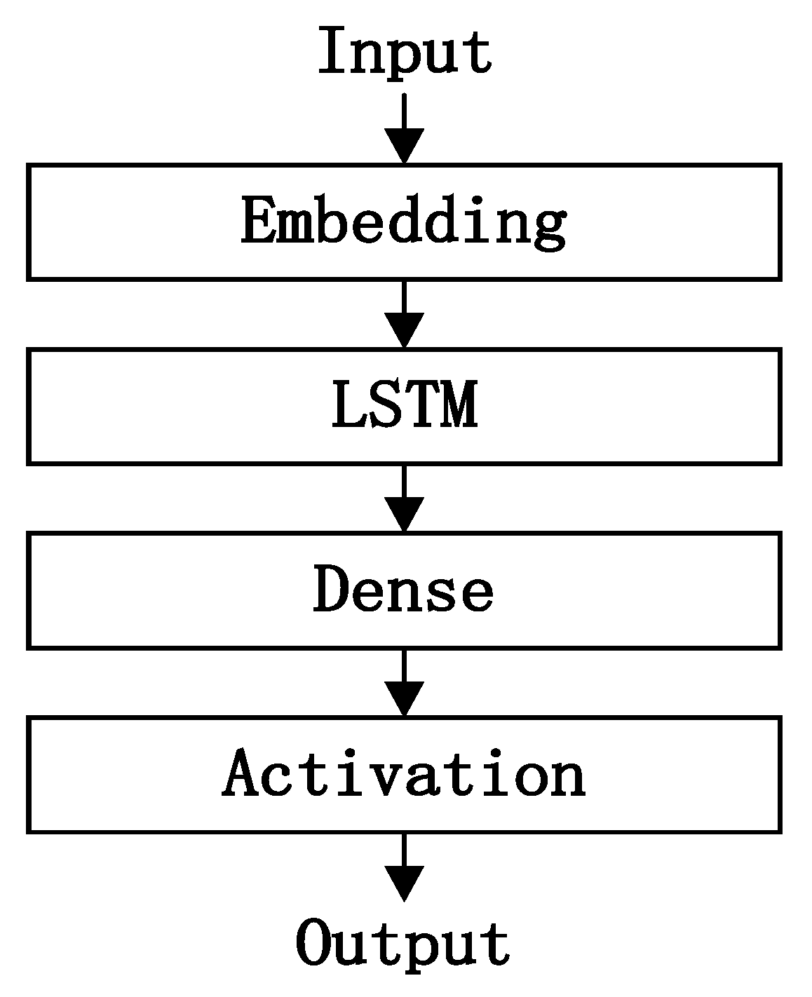
4.3. LSTM Model Training

The structure of the LSTM model used in this paper is shown in Figure 1, which includes an embedding layer, an LSTM layer, a dense layer, and an activation layer.

The embedding layer in Figure 1 maps the input sequence to a multidimensional feature space, forming an input matrix. The rows in the matrix represent the characters in the input sequence, and the list shows the dimensions of the feature space. The LSTM layer can implicitly extract advanced features from the sequence. The dense layer and activation layer complete the classification based on the extracted feature information and use the sigmoid function to compress the results to the range [0–1]. Finally, a prediction probability is output, representing the probability that the domain name belongs to a certain category. In this article, if the output probability is greater than or equal to 0.5, it indicates that the domain name is a DGA domain name, and vice versa, that it is a normal domain name.

This paper implemented an LSTM detection model based on the Keras framework, as shown in

Table 8. LSTM detect model code snippets.

model = Sequential()

model.add(Embedding(max_features,128, input_length=max_len))

mode1.add(LSTM(128))

model.add(Dropout(0.5))

mode1.add(Dense(1))

model.add(Activation(‘sigmoid’))

model.compile(loss=‘binary_crossentropy’, optimizer=‘adam’)

. In order to pursue better detection results, this paper used loss as a comparative indicator and a cross-validation to adjust the parameters in the LSTM layer.

Table 9. LSTM optimal parameter table (loss = 0.0529).

Parameter	Value	Parameter	Value
bacth_ size	128	epoch	10
max_feature	40	dropout	0.5
max_len	60	learning_rate	0.001
optimizer	adam

is the optimal parameter table for the LSTM detection model, with a maximum length of 60 for the input string. The input string was converted into an index value vector and input into the embedding layer. In the embedding layer, each character was mapped to a 128-dimensional embedding vector. In the selection section of the optimizer, experiments have shown that the Adam optimizer [38] can achieve a better loss convergence compared to RMSProp [22].

4.4. CNN Model Training

This paper used the open-source CNN detection model from reference [39] for DGA domain name detection, and the model structure is shown in Figure 2. The model code is shown in

Table 10. CNN model code snippets.

def getconvmodel(self, kernel_size, filters):

model = Sequential()

model.add(Conv1D(filters=filters, input_shape=(128,128), kernel_size=kernel_size,

padding=‘same’, activation=‘relu’, strides=1))

model.add(Lambda(lambda x: k.sum(x, axis=1), output_shape=(filters,)))

model.add(Dropout(0.5))

return model

main_input = Input(shape=(self.max_len,), dtype=‘int32’)

embedding = Embedding(input_dim=self.max_features, output_dim=128,

input_length=self.max_len)(main_input)

conv1 = self.getconvmodel(2,256)(embedding)

conv2 = self.getconvmodel(3,256)(embedding)

conv3 = self.getconvmodel(4,256)(embedding)

conv4 = self.getconvmodel(5,256)(embedding)

merged = Concatenate()([conv1, conv2, conv3, conv4])

middle = Dense(1024, activation=‘relu’)(merged)

middle = Dropout(0.5)(middle)

middle= Dense(1024, activation=‘relu’)(middle)

middle = Dropout(0.5)(middle)

output = Dense(1, activation=‘sigmoid’)(middle)

model = Model(inputs=main_input, outputs=output)

model.compile(loss=‘binary_crossentropy’, optimizer=’adam’)

return model

. The model uses the embedding layer to transform the input sequence into a distributed representation containing rich semantic information. The model adopts a parallel structure of multiple convolution layers, and the pooling operation is aimed at the entire domain name sequence, which makes the model only focus on whether there are patterns in the domain name but does not save its specific location information, so the model is robust to the insertion and deletion of characters, and subsequences that appear anywhere in the domain name sequence can be detected.

Table 11. CNN optimal parameter table (loss = 0.107).

Parameter	Value	Parameter	Value
bacth_ size	128	epoch	10
max_feature	40	dropout	0.5
max_len	60	learning_rate	0.001
optimizer	adam

shows the optimal parameter information of the CNN detection model, with loss as the comparison indicator and parameter adjustment using cross-validation. The input sequence was transformed into a 128-dimensional embedding vector in the embedding layer, and then a one-dimensional convolutional layer was used to extract local features of character sequences at different levels. All layers in the model except the input layer used Relu (rectified linear unit) as the activation function, the Adam optimizer was selected, and the parameter of the dropout was set to 0.5 [40], which destroyed the complex collaborative adaptation in the network and prevented overfitting.

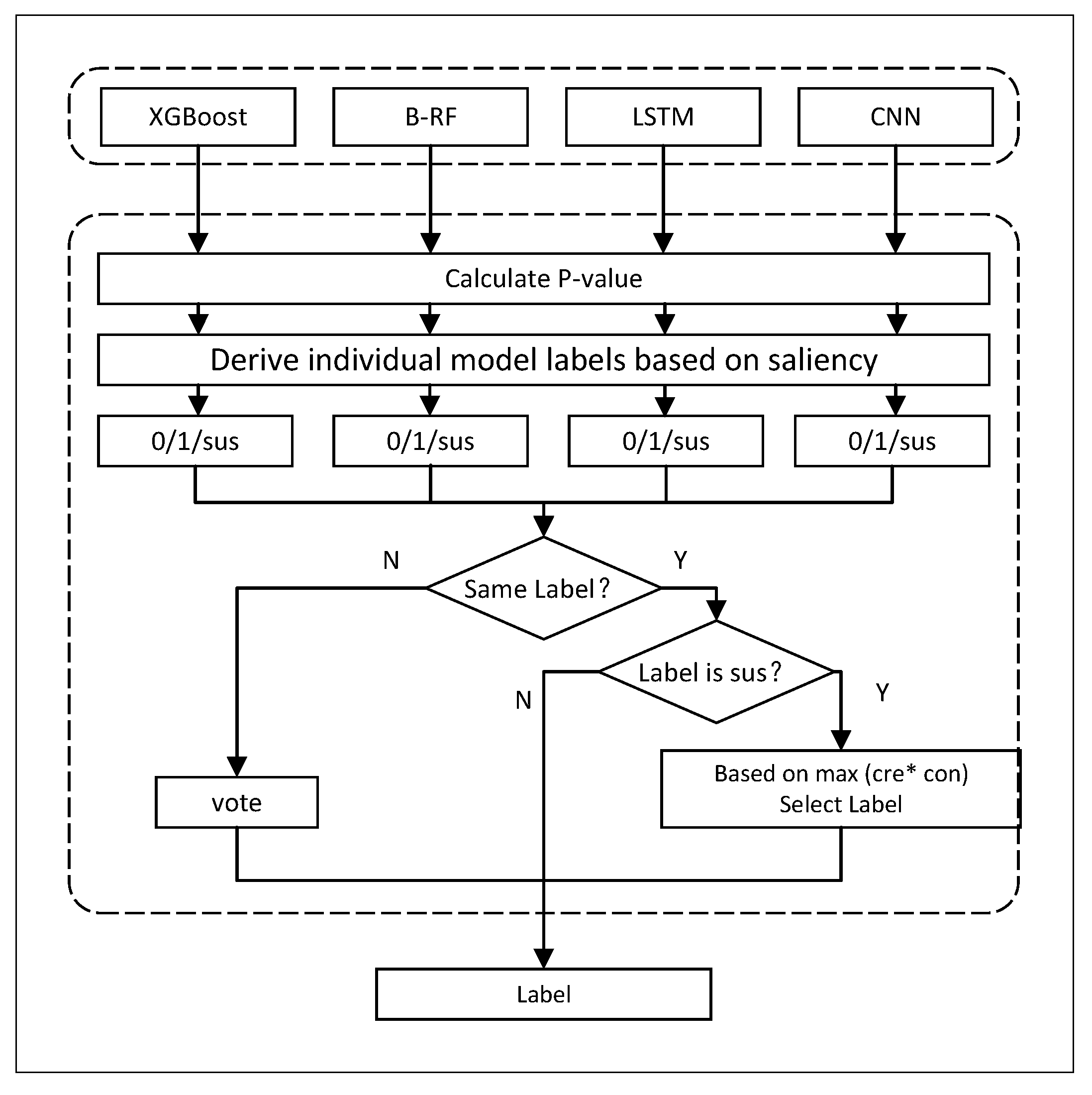
4.5. DGA Domain Name Detection Based on Statistical Learning

The main work of this section is to evaluate the prediction quality of the basic detection model based on the various basic detection models obtained in the previous text, using the conformal evaluator and significance evaluation. Based on the evaluation results, corresponding strategies are adopted to obtain the final label. Figure 3 is a multimodel decision flowchart based on statistical learning.

As shown in Figure 3, the decision-making mechanism can be divided into two parts: (1) determining the predictive labels of the basic model based on p-values and significance levels and (2) determining the final labels based on statistical analysis. Next, we elaborate on the implementation details of these two parts (In the figure, * represents product.).

4.5.1. Determining Basic Model Prediction Labels

When inputting a new test sample, the detection model first analyzes the sample using four basic models: XGBoost, B-RF, LSTM, and CNN. Each basic model outputs a probability score that represents the probability that the sample belongs to a certain class. Based on these probability scores, $p^l$, $l\in L$, and L representing all class labels of the sample in each class can be calculated. The following text provides a detailed explanation of the process of calculating the p-value.

For a binary classification task, $L=(0,1)$, assuming M is the DGA domain name sample set with sample labels of 1, and G is the normal domain name sample set with sample labels of 0. Using M and G to train the basic model A, after training, model A outputs a probability score for each DGA sample in M, forming a DGA sample score set $Scor{e}_M=\{{\alpha }_1,{\alpha }_2\dots {\alpha }_n\}$. Similarly, we generate a normal sample score set for the normal samples in $Scor{e}_G=\{{\beta }_1,{\beta }_2\dots {\beta }_n\}$. At this point, we input the sample point $z^{*}$ to be tested, and model A outputs its probability score $s^{*}$. Then, the $p^0$ and $p^1$ values of the sample point $z^{*}$ in model A are shown in Formulas (3) and (4).

$$\frac{p^0=\left|\{i=1,2\dots ,n|{\beta }_i\ge s^{*}\}\right|}{\left|n\right|},$$

(3)

$$\frac{p^1=\left|\{i=1,2\dots ,n|{\alpha }_i\le s^{*}\}\right|}{\left|n\right|}.$$

(4)

The range of probability scores is [0–1], and the larger the probability score, the more similar the sample is to the DGA sample. Therefore, the probability score of most samples in the normal domain name sample set G is closer to 0, and the smaller the value, the more normal the sample is. $p^0$ is equal to the proportion of samples in G with scores higher than $s^{*}$. This means that the larger the $p^0$, the more samples in G have scores higher than $z^{*}$, indicating that the fitting degree between $z^{*}$ and G is better than most samples, and $z^{*}$ and G have a higher similarity degree; for the malicious sample set, most samples have scores closer to 1, and the higher the probability score, the more malicious the samples are. Therefore, $p^1$ is equal to the proportion of samples in M with scores lower than $s^{*}$. The larger the $p^1$, the more similar $z^{*}$ is to M.

After obtaining the p-value, we use significance $\epsilon$ (maximum error probability) to divide the prediction labels of the basic model into acceptable and unacceptable. If $max(p^0,p^1)=p^0$ and $p^0\ge \epsilon$, then it means that the basic model A has a probability of at least $1-\epsilon$. The confidence level assumes that the sample label is 0, which is acceptable, ${Label}_A=0$. If $max(p^0,p^1)\le \epsilon$, the prediction quality of the basic model A for this sample is very low, exceeding the acceptable tolerance range. Therefore, the prediction result is rejected and marked as “suspicious”, ${Label}_A=suspicious$. The specific process is shown in Algorithm 1.

Algorithm 1: Determine a single model label based on p-value and confidence level $\epsilon$

Input: confidence level $\epsilon$ $p^0$, $p^1$ of the sample Output: $Labe{l}_{Model}$ 1: if $p^0>p^1$ and $p^0>\epsilon$ 2: $Labe{l}_{Model}=0$ 3: else if $p^1>p^0$ and $p^1>\epsilon$ 4: $Labe{l}_{Model}=1$ 5: else if $max(p^0,p^1)<\epsilon$ 6: rejecting predicted outcomes 7: $Labe{l}_{Model}=suspicious$

Unlike determining prediction labels based on probability and static thresholds, this method determines classification labels based on the overall fit between the sample and the sample set and introduces a significance level in the detection results of the basic model, further subdividing the detection results, so that the output results of the basic model have a certain level of confidence and improve the reliability of the results.

4.5.2. Multimodel Collaborative Prediction Based on Statistical Learning

After obtaining the label results of the basic model through the above steps, a set of basic model labels can be obtained. Next, a statistical analysis is conducted on this label set, and the final result is determined according to the following strategies.

• If the label results of all models are 1 or 0, it indicates that the decision results of all basic models are consistent and have a certain level of confidence in this result. Therefore, the label is directly output as the final result.
• If the label results of all models are “suspicious”, it indicates that the prediction quality of all models is lower than $\epsilon$. In this case, it is necessary to calculate the confidence and credibility values of each model for the sample based on the p-value and comprehensively evaluate the prediction quality of the basic model from two perspectives. When the confidence and credibility are both large, it indicates that the sample points are similar to the predicted category and have significant differences from other categories, indicating that the basic model has a higher classification quality for $z^{*}$. Therefore, this article used the product (cre * con) method to select the model with the highest quality from these basic models and uses the prediction label of this model as the final result.
• If the label results of all models are inconsistent, a vote is taken to determine the label (“suspicious” results are not included). If there is an equal number of votes, the final label is selected based on the combination of confidence and credibility.

In summary, in the multimodel collaborative decision-making section based on statistical learning, labels are determined based on the fitting degree between the samples and each type of sample set by calculating the p-value in the conditional evaluator, and a manually preset significance level $\epsilon$ is used to perform a secondary screening and partitioning on the prediction results of the basic model (0, 1, suspicious) and narrow the scope of suspicious results by statistically analyzing the set of basic model labels. When all models are unable to make predictions with a certain level of confidence, we evaluate the model results from the perspectives of confidence and credibility and make decisions. On the contrary, voting is used to obtain the final result. This decision-making method based on statistical learning provides the same comparison standard for heterogeneous methods, has wide applicability and good application prospects, and introduces significance and confidence levels in the decision-making process, making the prediction results more reliable.

5. Experimental Process and Results Analysis

This section is an experiment and validation of the DGA detection algorithm based on multiple models. This section first briefly introduces the experimental environment, experimental data, data preprocessing process, and evaluation indicators and then trains and tests the detection performance of the model using known sample data. The experimental environment used in this paper is shown in

Table 12. Experimental environment table.

CPU	4 cores
Memory	8G
Operating system	Ubuntu 16.04 64 bit
Python version	3.6
Python library version	tensorflow2.2.0, keras2.4.3

.

5.1. Experimental Data and Data Preprocessing

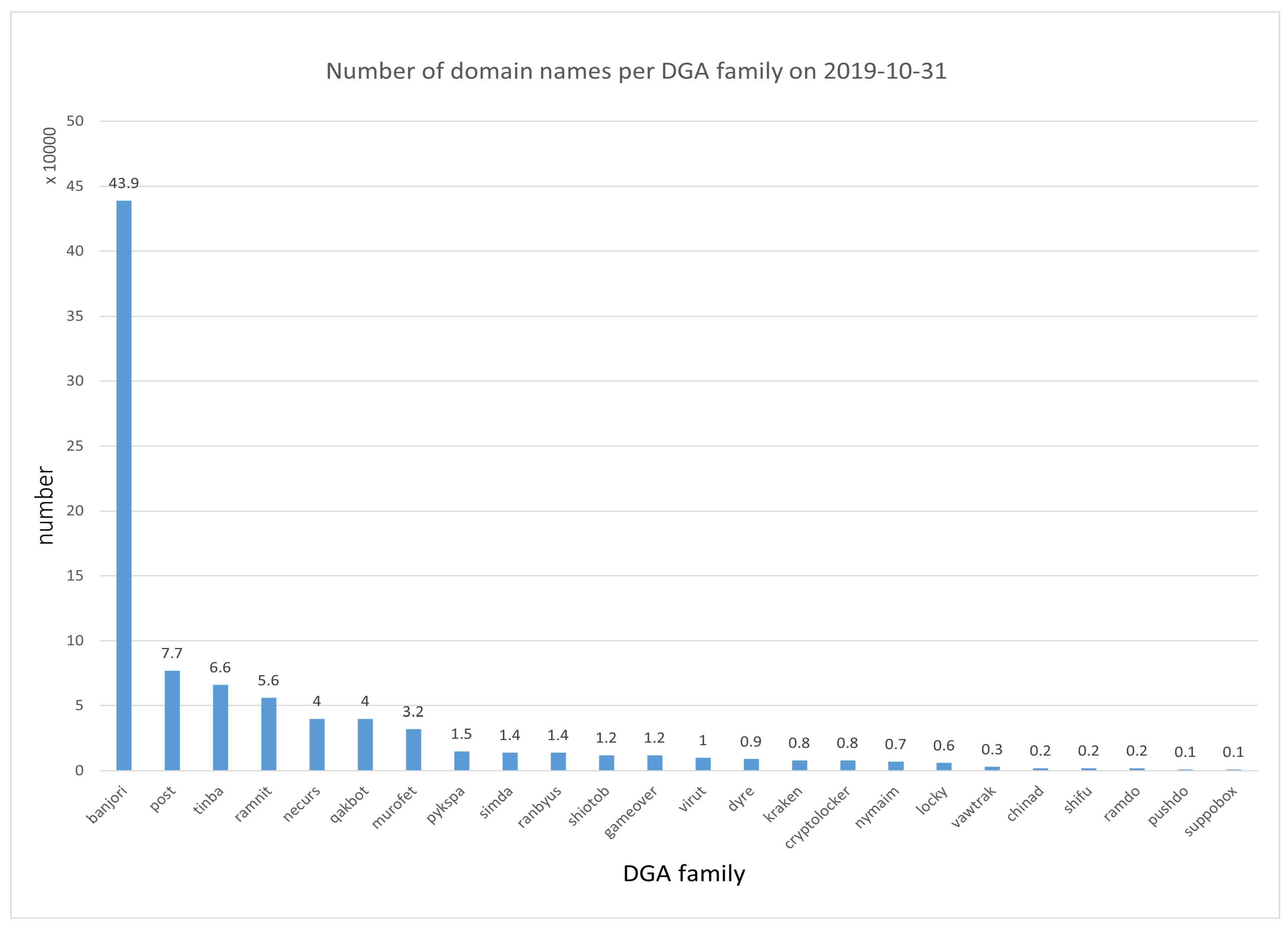
5.1.1. Dataset

The dataset used in this experiment included DGA domain name data obtained by crawlers and Tranco_K26W-1m, as shown in

Table 13. Experimental data table.

Dataset	Data Size
C_DGA	15,713,816
Tranco_K26W-1m	1,000,000

.

C_DGA: C_DGA is the latest published DGA domain name data obtained from multiple intelligence sources such as 360 and Bambenek using a crawler in this experiment. The C_DGA dataset includes DGA domain names published by various intelligence sources from 31 October 2019 to 17 May 2023. As of now, a total of 6,442,220 DGA domain names have been obtained. These domain names come from different DGA families. Taking 894,247 domain names obtained from 31 October 2019 as an example, they belong to 54 DGA families. Figure 4 shows the number of domain names in some of the DGA families.

Tranco_K26W-1m dataset: Although Alexa is the most commonly used whitelist, the literature [41] demonstrates that Alexa is highly susceptible to manipulation and contamination, which may have an impact on experimental results. Therefore, this paper selected the Tranco_K26W-1m dataset as the normal sample dataset, which was proposed by Le Pochat [41] to be formed by aggregating three commonly used whitelists, Alexa, Cisco Umbrella, and Majestic. These whitelists generate website rankings based on website traffic and popularity and then use the top-ranked domain names as whitelist data. However, the three are generated by different companies, so there are very few data that truly overlap. Therefore, the Tranco_K26W-1m label generated by the aggregation operation is more accurate and has a higher credibility.

5.1.2. Data Preprocessing

For all domain name data, we followed the following rules for data cleaning:

• Convert alphabetical characters in domain names to lowercase.
• Remove all domain names starting with “$xn$–”. Because a domain name starting with ‘$xn$–’ is an Internationalized Domain Name (IDN), the DGA algorithm will not generate an IDN domain name.
• Using “.” as a separator, remove domain names with more than four segments.
• Remove domain names from www.com and www.com.cn.
• Remove duplicate data.

Because most of the domain names generated by the DGA algorithm only generate intermediate domain name strings, and a complete domain name is formed after adding a top-level domain name, this experiment focused more on the secondary domain name and top-level domain name. If the domain name sample also contained subdomains such as a third-level domain name, this part of the character string was ignored, such as www.google.com, where only google.com was retained.

The DGA domain name samples and benign domain name samples used in this experiment are shown in

Table 14. Test sample information table.

DGA Domain Name Sample	Benign Sample
q4z1an1ca8icv1cl501sukun.biz	google.com
geb3jnercfn28qeq.org	facebook.com
1ihowds1u8fcu8kzuy549uytaj.com	windowsupdate.com
hpgkofoukqshvmt.info	yahoo.com

:

5.1.3. Evaluation Criteria

In the experiment, DGA domain names were defined as positive samples and normal domain names were defined as negative samples. The classification results of this experiment included the following four types, as shown in

Table 15. Confusion matrix table.

	Positive	Negative
True	TP (true positive)	TN (true negative)
False	FP (false positive)	FN (false negative)

in the confusion matrix.

• TP (true positive): it refers to the cases where the model correctly identifies a domain name as malicious, and it is indeed malicious.
• TN (true negative): it refers to the cases where the model correctly identifies a domain name as benign, and it is indeed benign.
• FP (false positive): it refers to the cases where the model incorrectly identifies a domain name as malicious, whereas it is actually benign.
• FN (false negative): it refers to the cases where the model incorrectly identifies a domain name as benign, whereas it is actually malicious.

This experiment was a dichotomous task with supervised learning. Therefore, accuracy, precision, recall, and F1 score were selected as evaluation criteria. Assuming that TP, TN, FP, and FN, respectively, represent the number of corresponding situations, the evaluation criteria are defined as follows:

• $Accuracy\left(ACC\right)$: represents the ratio of the number of correctly classified samples to the total number of samples.

  $$ACC=\frac{(TP+TN)}{(TP+TN+FP+FN)},$$

  (5)
• $Precision$: represents the ratio of the true number of positive samples to the number of positive samples in the classification results.

  $$Precision=\frac{TP}{(TP+FP)},$$

  (6)
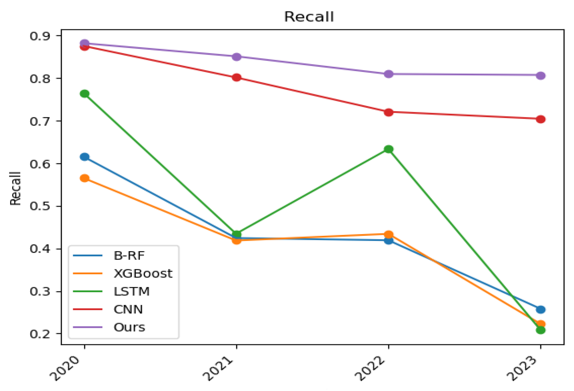
• $Recall$: represents the proportion of correctly classified positive samples to all positive samples, $Recall=TPR$.

  $$Recall=\frac{TP}{(TP+FN)},$$

  (7)
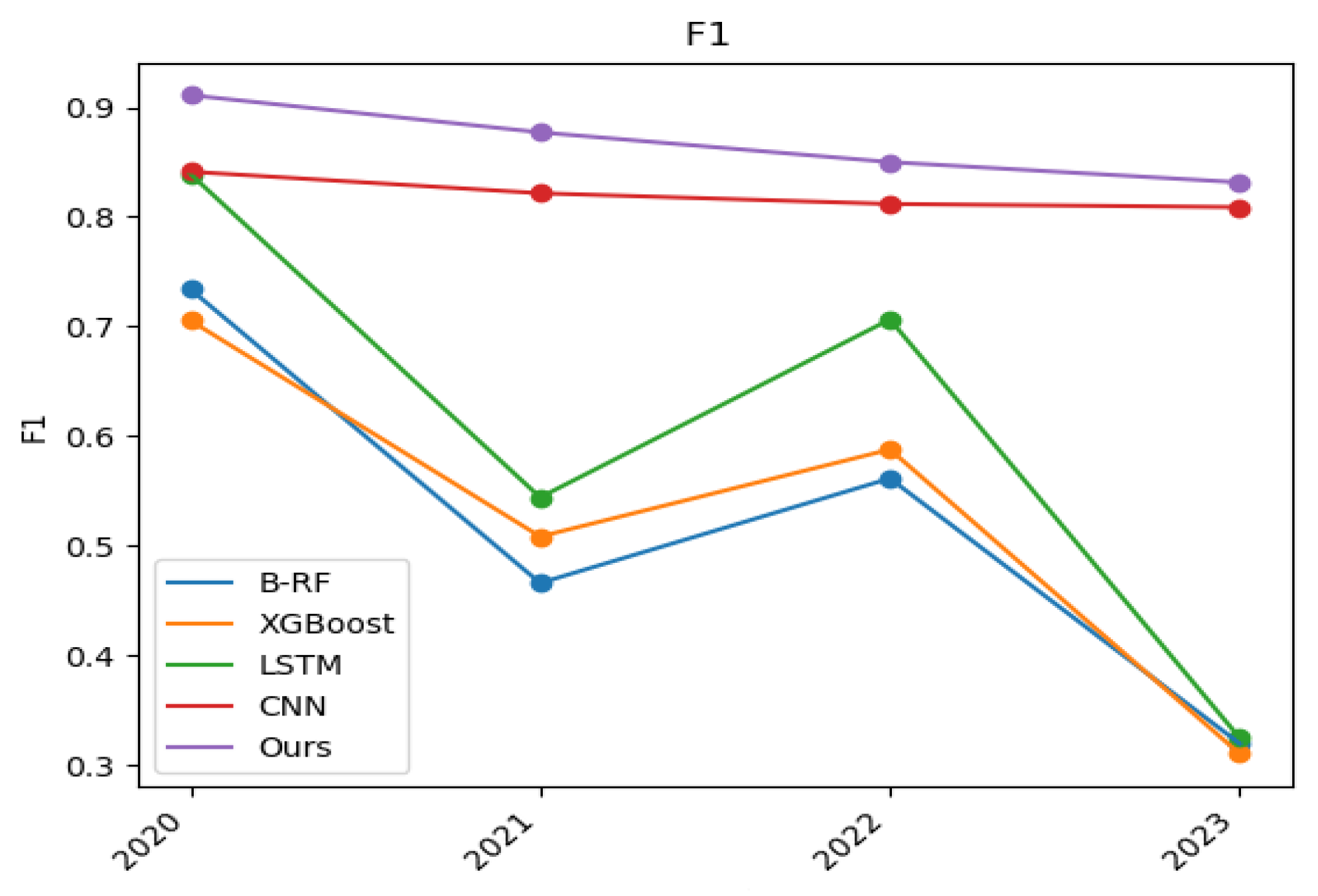
• $F1$: Represents the harmonic mean of the accuracy rate and the recovery rate. When the $F1$ value is high, it means that both the accuracy rate and the recovery rate are high.

  $$F1=\frac{(2\ast Precision\ast Recall)}{(Precision+Recall)}.$$

  (8)

For classification tasks, the higher the accuracy, precision, recall, and F1 values, the better the classification effect.

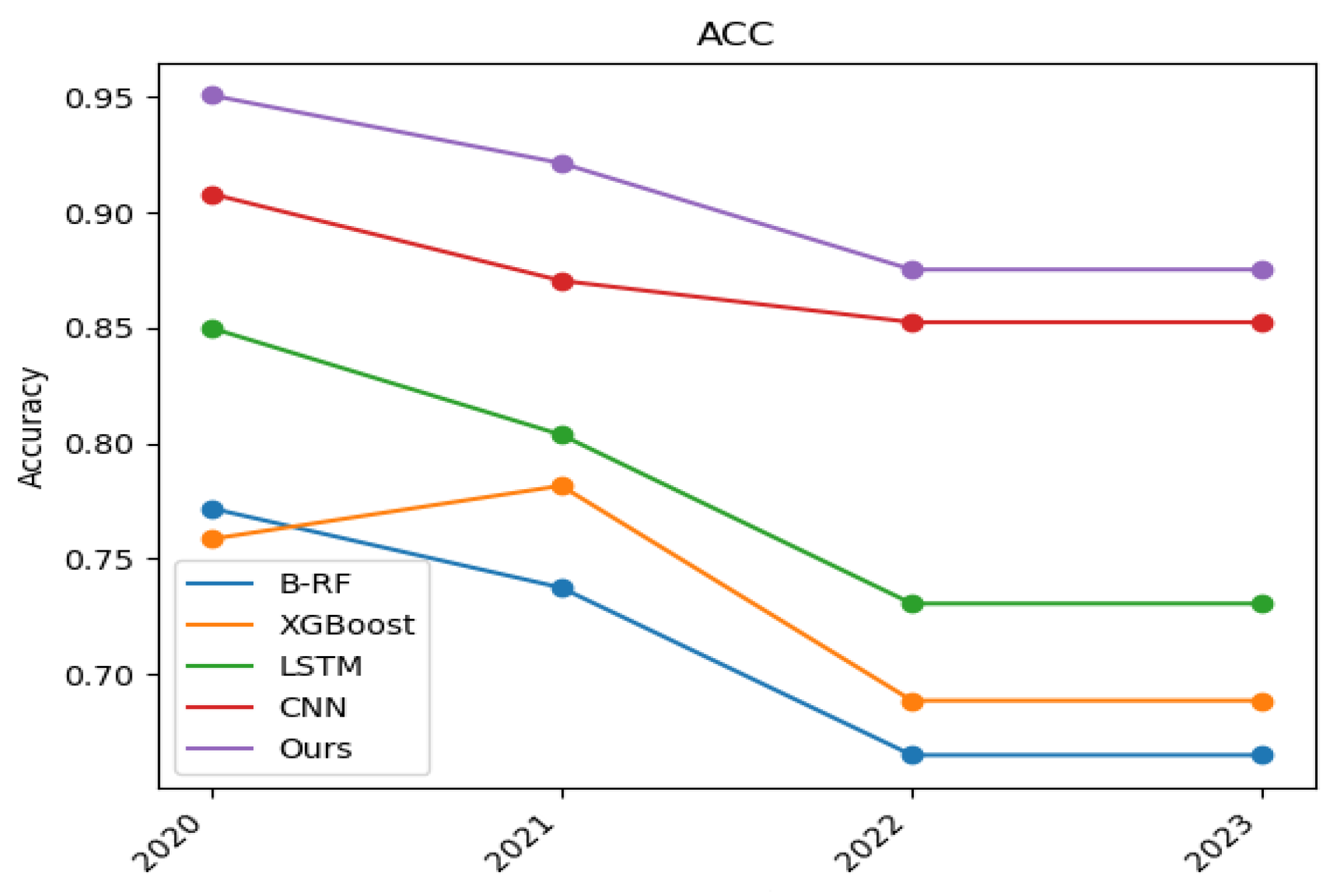
5.2. Experimental Results and Analysis

Experiment on C_DGA random sampling, compared to Tranco_K26W-1m, was merged as experimental data, and the training and testing sets were divided into a fivefold cross-validation ratio of 8:2. The specific information is shown in

Table 16. Training data and testing data size.

Dataset	Data Size
Training set	1,419,148
Testing set	354,788
Total	1,773,936

.

Using training data to train a statistical learning-based DGA detection model, the detection performance of the model was tested using test data and the four evaluation indicators mentioned above. The model was compared with multiple basic models, and the maximum fault tolerance rate was set to 0.01 in the experiment. The experimental results are shown in

Table 17. Table of experimental results for each model.

	Model Name	ACC	Precision	Recall	F1
1	B-RF	0.97551	0.96976	0.98063	0.97516
2	XGBoost	0.97554	0.96982	0.98062	0.97518
3	LSTM	0.97480	0.97066	0.979193	0.97490
4	CNN	0.96944	0.95212	0.98859	0.97001
5	B-RF + XGBoost	0.97498	0.97500	0.97496	0.97498
6	LSTM + CNN	0.97554	0.97613	0.97404	0.97833
7	B-RF + XGBoost + LSTM	0.97771	0.97498	0.98059	0.97778
8	B-RF + XGBoost + CNN	0.97768	0.97472	0.98081	0.97775
9	B-RF + LSTM + CNN	0.97791	0.97562	0.98032	0.97796
10	XGBoost + LSTM + CNN	0.97554	0.97661	0.97851	0.97756
11	XGBoost + B-RF + LSTM + CNN	0.97908	0.97712	0.98113	0.97912

. The boldface represents the highest value detected.

The first four rows in Table 17 represent the accuracy of traditional basic models B-RF and XGBoost, which was 0.97551 and 0754, respectively, slightly better than the detection accuracy of deep learning models LSTM and CNN, which was 0.97480 and 0.96944. The F1 values of traditional basic models B-RF and XGBoost were 0.97516 and 0.97518, which were also better than the F1 values of deep learning models of 0.97490 and 0.97001. This may be due to the more comprehensive and high-quality features selected in this paper, which better fit the dataset used in this paper and improved the detection performance of the traditional machine learning model. At the same time, due to the shorter length of the domain name, it belonged to a short text. Therefore, the hidden features that deep learning models can mine were limited, resulting in slightly lower performance than B-RF and XGBoost.

The 5th to 11th rows in Table 17 show the detection results of various combination models based on statistical learning decisions, such as LSTM + CNN representing the detection model based on statistical learning combined with LSTM and CNN. Comparing lines 3, 4, and 6, it can be found that the LSTM + CNN model outperformed the basic models LSTM and CNN in terms of accuracy, precision, and F1 value, indicating that the former had a higher comprehensive detection ability. For rows 1, 2, and 5, the B-RF + XGBoost model did not improve on the original foundation. This is because both B-RF and XGBoost are ensemble learning methods, and in this article, they were analyzed and trained on the same feature set. The two were relatively similar. When using significance level to subdivide the detection results in decision-making, the addition of the subclass class caused more noise in the B-RF + XGBoost method, which affected the detection performance of the B-RF + XGBoost model.

In addition, according to rows 5, 6, 7, 8, 9, 10, and 11 in observation Table 17, these combined models were superior to the basic model in accuracy, precision, and F1 value, which indicated that the decision-making mechanism based on statistical learning could effectively improve the detection effect on the basis of a single model. The detection performance of B-RF + XGBoost + LSTM and B-RF + XGBoost + CNN in the table was better than that of B-RF + XGBoost, while the detection performance of B-RF + LSTM + CNN and XGBoost + LSTM + CNN was better than that of LSTM + CNN. This indicates that the more types of basic models included in the detection model, the better the detection performance. When both machine learning methods based on artificial features and deep learning methods were included, the detection performance was better than only including one type of method.

The 11th row in Table 17 is the DGA detection model proposed in this article, which includes two machine learning methods based on artificial features and two deep learning methods, achieving a balanced state. By comparing with other models, it can be concluded that the detection model proposed in this paper outperformed the basic model in terms of accuracy, precision, and F1 value and was also superior to other combination models. In terms of recall index, it was only lower than the CNN model, indicating that the DGA detection model based on statistical learning had a stronger detection ability compared to these models.

DGA domain names belonged to different DGA families, so we used 360netlab’s DGA family domain name information to test the detection performance of the model for each family. During the experiment, one domain name of the DGA family was detected each time. As the test samples only contained positive samples, only accuracy was selected as the evaluation criterion. The experimental results are shown in

Table 18. The detection accuracy of each model for each DGA family.

DGA Family	Number	B-RF	XGBoost	LSTM	CNN	Ours
bamital	104	0.98076	0.94230	1.00000	1.00000	1.00000
conficker	497	0.73440	0.74849	0.75653	0.72434	0.77464
cryptolocker	1000	0.98700	0.98700	0.99100	0.98600	0.99400
dyre	1000	1.00000	1.00000	1.00000	0.99700	1.00000
emotet	446,590	0.99153	0.99074	0.99527	0.99521	0.99543
feodo	263	1.00000	0.99661	1.00000	1.00000	1.00000
fobber-v1	299	1.00000	1.00000	1.00000	1.00000	1.00000
gameover	12,000	1.00000	1.00000	0.99983	0.99981	1.00000
necurs	8188	0.94589	0.94687	0.95994	0.95346	0.96433
nymaim	478	0.82383	0.82642	0.82642	0.78497	0.86139
padcrypt	168	0.97619	0.97619	0.97023	0.96428	0.98809
pykspa-v1	44,702	0.89168	0.89224	0.96470	0.96085	0.96492
pykspa-v2-fake	800	0.86875	0.88250	0.84750	0.84000	0.89375
pykspa-v2-real	198	0.69697	0.83333	0.86868	0.84848	0.87878
ranbyus	10,920	0.99340	0.99322	0.99505	0.99587	0.99688
rovnix	179,991	0.98386	0.88268	0.99660	0.99745	0.99860
virut	9740	0.74589	0.76324	0.75657	0.71899	0.78839

, and the last column in the table represents the detection performance of the proposed model. From the table, it can be seen that the detection performance of the model on these DGA families was better than that of the basic model.

With the passage of time, DGAs are constantly evolving, and new DGA domain names appear every day, leading to the aging of DGA detection methods and a decrease in detection performance. Therefore, this paper used outdated data to train the detection model and tested the model’s detection performance over time on new data in the coming year.

In the experiment, data from the C_DGA dataset from 31 October 2019 to 28 December 2019 were extracted as DGA domain name samples for the training set, and Tranco_K26W-1m was used as the normal domain name sample for the training set. The experimental results are shown in Figure 5, Figure 6, Figure 7 and Figure 8. The blue curve represents the B-RF detection model, the orange curve represents XGBoost, the green curve represents the LSTM detection model, the red curve represents the CNN detection model, and the purple curve represents the DGA detection model based on statistical learning in this paper.

The accuracy of the four base models, as well as the detection model proposed in this paper at four time nodes are shown in Figure 5, from which it can be seen that the accuracy of the DGA detection model based on statistical learning is higher than that of the four base models, indicating that more samples were correctly categorized in the detection results of this model. Statistically based models show the highest accuracy among all models. This may be because the multimodel collaborative model combines the advantages of different models and improves the overall detection performance through ensemble learning. This result demonstrates the effectiveness and advantages of a model ensemble.

Figure 6 shows the variation of the precision rate of the base model and the statistical learning-based DGA detection model over four time nodes, from which it can be seen that the precision rate of the model detection decreases over time, which is caused by the degradation of the model. It can also be seen that the precision rate of CNN is significantly higher than that of other single-model detection but lower than that of statistically based multimodel detection. Thus, statistically based multimodel detection methods have a clear advantage.

Figure 7 demonstrates the variation of the recall of the base model and the statistical learning-based DGA detection model over the four time nodes. In terms of the single-model detection methods, the CNN model has a higher detection recall than the other three single-model detection methods. Due to the advantages of the CNN model in image processing and feature extraction, it can better capture and identify the characteristics of DGA attacks. These features include pattern recognition, frequency analysis, or other statistical features relevant to DGA attacks. However, it can be seen from the figure that the statistical learning-based DGA detection model has a higher recall than the CNN detection model at all time nodes. In summary, it can be seen that the statistical-based multimodel detection method has a higher recall than the other single-model detection methods.

Figure 8 demonstrates the variation of the F1 values of the base model and the statistical learning-based DGA detection model over the four time nodes, which is a combined assessment of precision and recall and responds to the comprehensive detection capability of the model. From the figure, it can be seen that the F1 value of the statistical learning-based DGA detection model is higher than the base model at all time nodes. Statistical learning-based DGA detection model may be better able to identify patterns, variants, and characteristics of DGA attacks, thereby improving the overall performance of the model. This indicates that the detection effect of the model is overall better than that of the base model.

In summary, when the detection model was trained with the outdated data and we tested the detection effect on the DGA domain name data for the next four years, the statistical learning-based DGA detection model outperformed the four base models in terms of accuracy, recall, and F1 value, which indicates that the detection model proposed in this paper possesses stronger comprehensive detection capability. When there were new DGA domain names that the model had not seen in the test data, the oscillation of the model on the four metrics was slightly lower than that of the other base models, which indicates that the detection model can effectively identify the internal aging models when making decisions based on statistical learning and eliminate the detection results of the less effective models according to various decision mechanisms, so that the overall detection effect of the whole model remains stable and has a certain degree of robustness.

5.3. Summary

This section validated the statistical learning-based DGA domain name detection algorithm proposed in the previous section through experiments. This section first utilized the C_DGA and Tranco_K26W-1m data to train and generate a statistical learning-based DGA detection model. Subsequently, the model’s classification ability was tested on the test set. The experimental results showed that the model outperformed the base model in three indexes of accuracy, precision, and F1 value, reaching values of 0.97908, 0.97712, and 0.97912, respectively, and the recall rate was also only lower than that of the CNN model, reaching 0.98113, indicating that the model had a stronger comprehensive detection ability than the other models. By comparing the base model and other combined models, we learned that the multimodel collaborative decision-making based on statistical learning proposed in this paper could effectively improve the detection effect on the basis of a single model, and the detection effect was better when the model contained both the base model based on artificial features and the base model based on deep learning. Next, this section tested the detection effect of this detection model for each DGA family using the DGA domain family data from 360netlab, and the experiments showed that the detection accuracy of our model on multiple DGA families was higher than that of the base model. Finally, we used the old data in C_DGA to generate detection models and test the detection effectiveness of these models over time, and the experimental results showed that in the time range from 2020 to 2023, the accuracy, recall, and F1 values of the statistical learning-based DGA detection model were higher than those of the base model, the comprehensive detection ability was stronger, and for unknown families of domain names, the detection model had less oscillation than the base model and had a certain robustness.

6. Conclusions and Future Work

6.1. Conclusions

This paper combined the analysis of artificial features and advanced neural network features to detect DGA domain names. First, 34 artificial features were extracted from the perspectives of string structure, language characteristics, and distribution statistics.

Secondly, deep neural networks were used to actively mine high-level features of domain name characters. Then, the DGA domain name was detected by combining traditional machine learning methods and deep learning methods. In terms of the multimodel decision-making mechanism, a method based on statistical learning was proposed to provide a fair comparison standard for heterogeneous models and produce decision results with a certain level of confidence through voting. When the prediction labels of all models lacked sufficient confidence, confidence and credibility were considered to comprehensively evaluate the prediction quality of the model, and the prediction result with the highest quality was selected as the final decision result.

Finally, a DGA detection algorithm based on statistical learning was designed and implemented using four heterogeneous methods, XGBoost, B-RF, LSTM, and CNN, to detect DGA domain names and evaluate the prediction quality of these methods through statistical learning to generate DGA detection results. This algorithm analyzed DGA domain names from multiple angles. The experimental results of this model performed well, with accuracy, precision, recall, and F1 scores reaching 0.979, 0.977, 0.981, and 0.979. Our research was compared with previous studies and discussed with related studies. We found that our method outperformed the performance of a previously proposed single model, improved the detection effect based on a single method, and was able to effectively identify invalid prediction results, ensuring the stability of the algorithm. Overall, this algorithm is a real-time, lightweight DGA detection method with high accuracy and reliability.

6.2. Future Work

In this paper, a statistical learning-based DGA detection method was proposed, but due to the limited research time, there are still some problems that need further research and improvement:

• The detection method proposed in this paper contains four heterogeneous methods, XGBoost, B-RF, LSTM, and CNN, and provides a unified comparison standard for these heterogeneous models using statistical learning, which has strong scalability and provides a new way of thinking for multimodel detection of DGA domain names, so more and better detection methods can be considered for integration into this algorithm in future research to further improve the detection capability of the algorithm.
• In this paper, we studied the binary classification problem in DGA detection, and in future research, we can try to apply this detection algorithm to the DGA family multiclassification problem. By extending the algorithm to classify different DGA families, a more comprehensive understanding of the diverse nature of DGA domains can be achieved.
• Incorporating explainability: In future research, it would be valuable to enhance the interpretability and explainability of the detection algorithm. By providing insights into the decision-making process of the model and the importance of different features, users can gain a better understanding of how the algorithm detects DGA domains.
• Real-time detection: This study mainly focuses on offline detection of DGA domains. In future research, it would be beneficial to explore real-time detection methods that can effectively identify DGA domains in a timely manner. This would enable the algorithm to be deployed in dynamic environments, such as network security systems, where quick detection and response are crucial.
• Robustness to adversarial attacks: Investigating the robustness of the detection algorithm against adversarial attacks would be an important direction for future research. Adversarial attacks aim to deceive the algorithm by introducing subtle modifications to the input data. Developing techniques to enhance the algorithm’s resilience to such attacks would be valuable in practical applications.

References

1. Wagan, A.A.; Li, Q.; Zaland, Z.; Marjan, S.; Bozdar, D.K.; Hussain, A.; Mirza, A.M.; Baryalai, M. A Unified Learning Approach for Malicious Domain Name Detection. Axioms 2023, 12, 458. [Google Scholar] [CrossRef]
2. Chen, S.; Lang, B.; Chen, Y.; Xie, C. Detection of Algorithmically Generated Malicious Domain Names with Feature Fusion of Meaningful Word Segmentation and N-Gram Sequences. Appl. Sci. 2023, 13, 4406. [Google Scholar] [CrossRef]
3. Wang, H.; Tang, Z.; Li, H.; Zhang, J.; Cai, C. DDOFM: Dynamic malicious domain detection method based on feature mining. Comput. Secur. 2023, 130, 103260. [Google Scholar] [CrossRef]
4. Abu Al-Haija, Q.; Alohaly, M.; Odeh, A. A Lightweight Double-Stage Scheme to Identify Malicious DNS over HTTPS Traffic Using a Hybrid Learning Approach. Sensors 2023, 23, 3489. [Google Scholar] [CrossRef]
5. Zhou, J.; Cui, H.; Li, X.; Yang, W.; Wu, X. A Novel Phishing Website Detection Model Based on LightGBM and Domain Name Features. Symmetry 2023, 15, 180. [Google Scholar] [CrossRef]
6. Liang, Y.; Cheng, Y.; Zhang, Z.; Chai, T.; Li, C. Illegal Domain Name Generation Algorithm Based on Character Similarity of Domain Name Structure. Appl. Sci. 2023, 13, 4061. [Google Scholar] [CrossRef]
7. Wei, L.; Wang, L.; Liu, F.; Qian, Z. Clustering Analysis of Wind Turbine Alarm Sequences Based on Domain Knowledge-Fused Word2vec. Appl. Sci. 2023, 13, 10114. [Google Scholar] [CrossRef]
8. Chaganti, R.; Suliman, W.; Ravi, V.; Dua, A. Deep learning approach for SDN-enabled intrusion detection system in IoT networks. Information 2023, 14, 41. [Google Scholar] [CrossRef]
9. Rahali, A.; Akhloufi, M.A. MalBERTv2: Code Aware BERT-Based Model for Malware Identification. Big Data Cogn. Comput. 2023, 7, 60. [Google Scholar] [CrossRef]
10. Zhai, Q.; Zhu, W.; Zhang, X.; Liu, C. Contrastive refinement for dense retrieval inference in the open-domain question answering task. Future Internet 2023, 15, 137. [Google Scholar] [CrossRef]
11. Antonakakis, M.; Perdisci, R.; Nadji, Y.; Vasiloglou, N.; Abu-Nimeh, S.; Lee, W.; Dagon, D. From Throw-Away Traffic to Bots: Detecting the Rise of DGA-Based Malware. In Proceedings of the 21st USENIX Security Symposium (USENIX Security 12), Bellevue, WA, USA, 8–10 August 2012; pp. 491–506. [Google Scholar]
12. Plohmann, D.; Yakdan, K.; Klatt, M.; Bader, J.; Gerhards-Padilla, E. A Comprehensive Measurement Study of Domain Generating Malware. In Proceedings of the 25th USENIX Security Symposium (USENIX Security 16), Austin, TX, USA, 10–12 August 2016; USENIX Association: Austin, TX, USA, 2016; pp. 263–278. [Google Scholar]
13. Al lelah, T.; Theodorakopoulos, G.; Reinecke, P.; Javed, A.; Anthi, E. Abuse of Cloud-Based and Public Legitimate Services as Command-and-Control (C&C) Infrastructure: A Systematic Literature Review. J. Cybersecur. Priv. 2023, 3, 558–590. [Google Scholar]
14. Sui, Z.; Shu, H.; Kang, F.; Huang, Y.; Huo, G. A Comprehensive Review of Tunnel Detection on Multilayer Protocols: From Traditional to Machine Learning Approaches. Appl. Sci. 2023, 13, 1974. [Google Scholar] [CrossRef]
15. Zhang, C.; Chen, Y.; Liu, W.; Zhang, M.; Lin, D. Linear Private Set Union from Multi-Query Reverse Private Membership Test. In Proceedings of the 32nd USENIX Security Symposium (USENIX Security 23), Anaheim, CA, USA, 9–11 August 2023; pp. 337–354. [Google Scholar]
16. Eltahlawy, A.M.; Aslan, H.K.; Abdallah, E.G.; Elsayed, M.S.; Jurcut, A.D.; Azer, M.A. A Survey on Parameters Affecting MANET Performance. Electronics 2023, 12, 1956. [Google Scholar] [CrossRef]
17. Ogundokun, R.O.; Arowolo, M.O.; Damaševičius, R.; Misra, S. Phishing Detection in Blockchain Transaction Networks Using Ensemble Learning. Telecom 2023, 4, 279–297. [Google Scholar] [CrossRef]
18. Bubukayr, M.; Frikha, M. Effective Techniques for Protecting the Privacy of Web Users. Appl. Sci. 2023, 13, 3191. [Google Scholar] [CrossRef]
19. Davuth, N.; Kim, S.R. Classification of malicious domain names using support vector machine and bi-gram method. Int. J. Secur. Its Appl. 2013, 7, 51–58. [Google Scholar]
20. Vinayakumar, R.; Soman, K.; Poornachandran, P.; Sachin Kumar, S. Evaluating deep learning approaches to characterize and classify the DGAs at scale. J. Intell. Fuzzy Syst. 2018, 34, 1265–1276. [Google Scholar] [CrossRef]
21. Mowbray, M.; Hagen, J. Finding domain-generation algorithms by looking at length distribution. In Proceedings of the 2014 IEEE International Symposium on Software Reliability Engineering Workshops, Naples, Italy, 3–6 November 2014; pp. 395–400. [Google Scholar]
22. Woodbridge, J.; Anderson, H.S.; Barford, P. Inferring domain generation algorithms with a Viterbi algorithm variant. In Proceedings of the 2016 ACM SIGSAC Conference on Computer and Communications Security, Vienna, Austria, 24–28 October 2016; pp. 1010–1021. [Google Scholar] [CrossRef]
23. Schüppen, S.; Teubert, D.; Herrmann, P.; Meyer, U. FANCI: Feature-based Automated NXDomain Classification and Intelligence. In Proceedings of the 27th USENIX Security Symposium (USENIX Security 18), Baltimore, MD, USA, 15–17 August 2018; USENIX Association: Baltimore, MD, USA, 2018; pp. 1165–1181. [Google Scholar]
24. Yu, S.; Wu, J.; Xiang, Y. A novel method for DGA domain name detection based on character n-gram and sequence pattern. Secur. Commun. Netw. 2017, 2017, 4176356. [Google Scholar]
25. Yadav, S.; Reddy, A. Detecting algorithmically generated domain names with entropy-based features. In Proceedings of the 2013 ACM conference on Computer and Communications Security, Berlin, Germany, 4–8 November 2013; pp. 447–458. [Google Scholar] [CrossRef]
26. Zhao, D.; Li, H.; Sun, X.; Tang, Y. Detecting DGA-based botnets through effective phonics-based features. Future Gener. Comput. Syst. 2023, 143, 105–117. [Google Scholar] [CrossRef]
27. Bilge, L.; Balduzzi, M.; Kirda, E. Dissecting Android malware: Characterization and evolution. In Proceedings of the 2011 IEEE Symposium on Security and Privacy, Oakland, CA, USA, 22–25 May 2011; pp. 95–110. [Google Scholar] [CrossRef]
28. Kolias, C.; Kambourakis, G.; Stavrou, A.; Gritzalis, D. Detecting DGA-based botnets using DNS traffic analysis. IEEE Trans. Dependable Secur. Comput. 2016, 13, 218–231. [Google Scholar]
29. Zhao, C.; Zhang, Y.; Wang, Y. A Feature Ensemble-based Approach to Malicious Domain Name Identification from Valid DNS Responses. In Proceedings of the 2020 International Joint Conference on Neural Networks (IJCNN), Glasgow, UK, 19–24 July 2020; pp. 1–7. [Google Scholar]
30. Zhao, N.; Jiang, M.; Zhang, X.; Liu, Y. Detection of DGA domains using deep learning. In Proceedings of the 2018 15th IEEE International Conference on Advanced Video and Signal Based Surveillance (AVSS), Auckland, New Zealand, 27–30 November 2018; pp. 1–6. [Google Scholar]
31. Zhang, Q.; Ma, W.; Wang, Y.; Zhang, Y.; Shi, Z.; Li, Y. Backdoor attacks on image classification models in deep neural networks. Chin. J. Electron. 2022, 31, 199–212. [Google Scholar] [CrossRef]
32. Zheng, J.; Zhang, Y.; Li, Y.; Wu, S.; Yu, X. Towards Evaluating the Robustness of Adversarial Attacks Against Image Scaling Transformation. Chin. J. Electron. 2023, 32, 151–158. [Google Scholar] [CrossRef]
33. Sun, X.; Yang, J.; Wang, Z.; Liu, H. Hgdom: Heterogeneous graph convolutional networks for malicious domain detection. In Proceedings of the NOMS 2020-2020 IEEE/IFIP Network Operations and Management Symposium, Budapest, Hungary, 20–24 April 2020; pp. 1–9. [Google Scholar]
34. Li, C.; Xie, J.; Cheng, Y.; Zhang, Z.; Chen, J.; Wang, H.; Tao, H. Research on the Construction of High-Trust Root Zone File Based on Multi-Source Data Verification. Electronics 2023, 12, 2264. [Google Scholar] [CrossRef]
35. Li, X.; Lu, C.; Liu, B.; Zhang, Q.; Li, Z.; Duan, H.; Li, Q. The Maginot Line: Attacking the Boundary of {DNS} Caching Protection. In Proceedings of the 32nd USENIX Security Symposium (USENIX Security 23), Anaheim, CA, USA, 9–11 August 2023; pp. 3153–3170. [Google Scholar]
36. Ashiq, M.I.; Li, W.; Fiebig, T.; Chung, T. You’ve Got Report: Measurement and Security Implications of {DMARC} Reporting. In Proceedings of the 32nd USENIX Security Symposium (USENIX Security 23), Anaheim, CA, USA, 9–11 August 2023; pp. 4123–4137. [Google Scholar]
37. Xu, C.; Zhang, Y.; Shi, F.; Shan, H.; Guo, B.; Li, Y.; Xue, P. Measuring the Centrality of DNS Infrastructure in the Wild. Appl. Sci. 2023, 13, 5739. [Google Scholar] [CrossRef]
38. Glorot, X.; Bengio, Y. Understanding the difficulty of training deep feedforward neural networks. In Proceedings of the Thirteenth International Conference on Artificial Intelligence and Statistics, JMLR Workshop and Conference Proceedings, Sardinia, Italy, 13–15 May 2010; pp. 249–256. [Google Scholar]
39. Yu, B.; Gray, D.L.; Pan, J.; Cock, M.D.; Nascimento, A.C.A. Inline DGA Detection with Deep Networks. In Proceedings of the IEEE International Conference on Data Mining Workshops, Orleans, LA, USA, 18–21 November 2017. [Google Scholar]
40. Srivastava, N.; Hinton, G.; Krizhevsky, A.; Sutskever, I.; Salakhutdinov, R. Dropout: A simple way to prevent neural networks from overfitting. J. Mach. Learn. Res. 2014, 15, 1929–1958. [Google Scholar]
41. Pochat, V.L.; Van Goethem, T.; Tajalizadehkhoob, S.; Korczyński, M.; Joosen, W. Tranco: A research-oriented top sites ranking hardened against manipulation. arXiv 2018, arXiv:1806.01156. [Google Scholar]
Figure 1. LSTM model architecture.
Electronics 12 04121 g001
Figure 2. CNN model.
Electronics 12 04121 g002
Figure 3. Multimodel decision flowchart based on statistical learning.
Electronics 12 04121 g003
Figure 4. Number of domain names in partial DGA families (31 October 2019).
Electronics 12 04121 g004
Figure 5. Accuracy versus time.
Electronics 12 04121 g005
Figure 6. Precision versus time.
Electronics 12 04121 g006
Figure 7. Recall versus time.
Electronics 12 04121 g007
Figure 8. F1 versus time.
Electronics 12 04121 g008