Abstract
Owning to the application of artificial intelligence and big data analysis in industry, automobiles, aerospace, and other fields, the high-bandwidth candidate, time-sensitive networking (TSN), is introduced into the data communication network. Apart from keeping the safety-critical and real-time requirements, it faces challenges to satisfy large traffic transmission, such as sampled video for computer vision. In this paper, we consider task scheduling and time-sensitive network together and formalize them into a first-order-constraints satisfy module theory (SMT) problem. Based on the result of the solver, we build flow-level scheduling based on IEEE 802.1 Qbv. By splitting the flow properly, it can reduce the constraint inequality as the traffic grows more than the traditional frame-based programming model and achieve near 100% utilization. It can be a general model for the deterministic task and network scheduling design.
1. Introduction
It has been globally recognized that the construction of an intelligent industrial Internet will significantly enhance society as a whole. One key enabling technology is ensuring smooth production pipeline operations as machines are interconnected akin to the Internet. Deterministic design is a fundamental requirement where data must be sent, received, and operated on in a timely manner without ambiguity, including for both hard and soft real-time applications such as motion control, equipment manufacturing, and self-driving.
Traditional industrial networks separately consider communication and computing, with a focus on real-time execution of task scheduling on the CPU (central processing unit) and treat the network as a transparent substrate. The upper layer logic entrusts all communication support to the best effort (BE) network after establishing coarse time precision. Logic is highly reliant on communication for the correctness of the logic, with a few mistakes. For example, consistency or Byzantine problems are the primary focus of applications that relax network time precision to a second or minute level to ensure such correctness.
Additionally, the lack of semantic abstraction in the substrate layer can hinder fine-grained time control (microseconds to milliseconds) due to queuing strategies. For example, regardless of how many new versions of TCP (transmission control protocol), such as New Nano, Cubic, and BBR New Nano, Cubic, and BBR are commonly used in TCP, the classic three-way handshake is always employed. All entities engage in non-cooperative competition, with the whole network fluctuating around a Nash equilibrium [1]. Therefore, integrated consideration of communication and computing has become an important candidate for achieving microsecond to millisecond precision control.
With regard to communication, TSN [2,3,4] strives to establish a deep interconnection between the industrial network and the current Internet. The latter’s ecosystem, high bandwidth, and generality bring endless opportunities for the former’s development. One benefit of TSN is the flexibility it offers in terms of business support, as it can accommodate both real-time and BE messages. Another benefit is the high bandwidth capacity that allows for a wider variety of traffic. For example, autonomous vehicles require action after the computer vision process involving video sampled by the camera, which generates traffic several orders of magnitude higher than traditional industrial messages, i.e., CAN [5], Flexray [6], Lin [7], EtherCat, and TTE (time-triggered ethernet) [8] (each message is approximately 30∼500 bytes). Currently, the main challenge in applying TSN is the complex scheduling mechanisms [9], including the fundamental standard 802.1 Qbv, which attempts to design the gate-control list of each switch to meet strict delay and jitter requirements.
Turning to computing, real-time task scheduling is a historically mature topic [10,11,12]. RMS (rate monotonic scheduling), EDF (earliest deadline first), LLF (least slack first), and other classic algorithms have been integrated into real-time operating systems (RTOS), which can provide excellent real-time computing capabilities. However, there is still a gap between task scheduling and TSN when combining them for end-to-end scheduling. Although Craciunas et al. [13] began to combine tasks with TTE based on the assumption that one time-triggered frame is assigned to one task and shares the same period, and it can achieve excellent end-to-end delay and jitter control, it has two disadvantages. Firstly, it inherits the low bandwidth utilization of TTE; secondly, its frame-based programming model based on SMT (satisfy module theory) hardly supports large traffic tasks, where the NP-hard computation cost of SMT makes it hardly acceptable when the number of frames is larger than 10,000. Therefore, based on a similar idea, this paper proposes replacing TTE with TSN and proposes joint scheduling of both time-sensitive tasks and the network. Moreover, Refs. [14,15,16,17] have carried out corresponding work in joint task and network scheduling. One class of methods is based on flow control strategies, adjusting the network traffic to meet task requirements. Another type of method focuses on task scheduling, selecting the optimal execution order based on task characteristics and network status. There are also methods that combine flow control and task scheduling strategies to achieve more comprehensive optimization. However, these kinds of ‘jointing’ take more attention with respect to the task and, we must consider how to adjust the network to satisfy the requirement. In our work, we can elevate the scheduling granularity of TSN data transmission from the frame level to the flow level, which can establish a one-to-one correspondence between the time control granularity of the task level and the granularity of network transmission, and has potential cross-layer transmission capabilities
Our main contributions are as follows.
- We propose a novel periodic flow split theory and method that enables the mixed transmission of both periodic large and small flows while achieving near-100% bandwidth utilization with appropriate jitter control.
- We introduce a flow-based SMT programming model and enumerate the corresponding first-order logical constraints. The scheduling unit is flow-level, while the identification unit is frame-level, enabling the support of larger-scale SMT solutions.
- We map the transmission data of tasks into flow-level or split-flow-level gates. This approach allows tasks to label their data and track them in each device, potentially providing a new paradigm for application design.
The remainder of this paper is organized as follows:
Section 2 provides the background information and definitions of key terminology. Section 3 presents the flow-level scheduling model. Section 4 formulates the corresponding constraints. Section 6 demonstrates the experiment results and discussion of the proposed model. Section 7 summarizes the related works. Finally, Section 8 concludes this work and outlines future work.
2. System Model and Terminology
2.1. Joint Programming Model
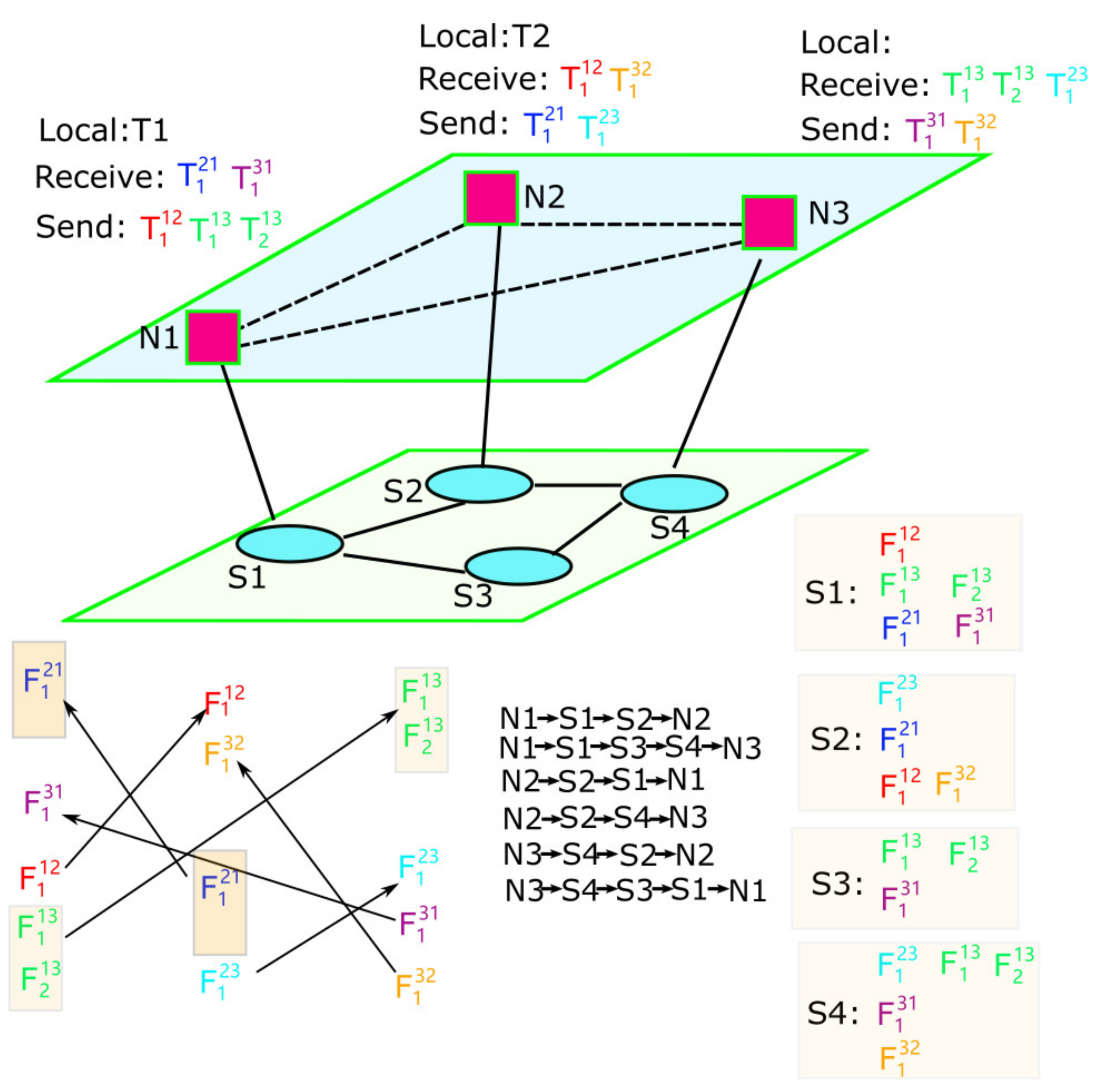
Figure 1 depicts the logical model, where the upper layer contains real-time computing nodes and the lower layer contains TSN switch nodes. The topological structure is abstracted as a directed graph , where the vertex set , N represents the set of computing nodes, S is the set of switch nodes and E is the set of directed links connecting nodes in V. Each link is denoted by pair of nodes , indicating the direction from to . denote the flow path composed of the ordered sequence of links between and . For instance,
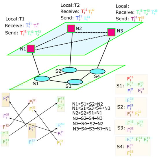
Figure 1.
Joint programming model of task and flow.
For simplicity, it can also be represented as an ordered sequence of nodes,
Let denote the set of all the paths that have data transmission.
2.2. Time Sensitive Task and Flow Formulation
Assume all the tasks are generated by the computing nodes, we define as the set of live tasks at time t; when changes, the scheduling strategy must also be adjusted. Each task has a life cycle characterized by the start time and end time . In the majority of this paper, we focus on a relatively stable environment where remains constant in a long term, and can be simply denoted as .
Real-time systems typically involve periodic and aperiodic tasks. Aperiodic tasks can be classified into deadline-constrained and best effort (BE) tasks. The key to optimal scheduling lies in periodic and deadline-constrained aperiodic task scheduling. Therefore, our focus is on how to optimally schedule these types of tasks. We use and to denote the set of periodic task and deadline-constraint aperiodic tasks, respectively. For , the tuple denotes the offset in each period, WCET (worst-case execution time), deadline and period. This 4-ary tuple can also represent the characteristics of tasks in and BE tasks. For , we set .
represents the task set executed on node , which includes local tasks , input tasks and output tasks . Each task in generates a data flow sent to other nodes, and denotes the flow from node to node . Let denote the flow set on . There is a bijective relationship between the task and flow, represented by , such that the flow set on node is and flow generated by task is . We inherit the 4-ary tuple to denote the offset in each period, the transmission time, deadline, and period, where . Generally, because the flow deadline has little impact on the task deadline and every flow can finish transmission within its period to avoid piling up. Let and denote the flow set and the flow on link , respectively. Note that in our figures and theoretical descriptions, we use and instead of and for simplicity; if there is any confusion, please treat the two as equivalent. Additionally, we stipulate that all periods within the same set are distinct because all flows with the same period can be bundled into one flow for scheduling.
Let denotes the set of destination nodes that node will send data flow to and denotes the set of source nodes that node will receive data flow from. Our objective is that every task T can be executed in real-time smoothly and can be transmitted through the network deterministically and timely. The core question is how to schedule all the tasks and flows properly. Owing to the different requirements, we should first judge the schedulability and then give a related schedule strategy. We have the following definitions.
Definition 1 (task schedulable).
If task can be executed in node within the constraints, we say T is task schedulable in .
Definition 2 (flow schedulable).
If flow can obtain within the constraints, we say is flow schedulable.
Definition 3 (end-to-end schedulable).
For node pair (, ), we say task T can be end-to-end schedulable if T and is task schedulable in and , respectively, and is flow schedulable.
Definition 4 (computing node schedulable).
If are task schedule, we say the node is computing node schedulable.
Definition 5 (holistic schedulable).
The system is holistically schedulable if are computing node schedulable and are end-to-end schedulable.
According to the definition, our target is to design a holistic schedulable system. However, unlike the loosely coupled traditional Internet, many scenarios in the industrial Internet are tightly coupled. Owing to the task growth and resource limit, maximizing utilization is a big challenge. We first pay more attention to the real-time transmission and later make a joint optimization by combining both of them by building a connection between the time of task scheduling and the network.
3. Flow-Based Deterministic Scheduling
In the traditional industrial scenario, the instruction set of the servo/PLC (programming logic controller) has complete semantics, and one instruction can be encapsulated into one frame whose size is from 32 to 500 Bytes. The frame is non-preemptive and TTE/CAN/Lin is enough. While in the self-driving scenario, for instance, there are about several megabytes (MB) of video for every 33 ms from the camera, there are 100 bytes of detection signal for every 31 μs from Ladar [6]. To the best of our knowledge, they are always handled by hard slice isolation based on TDM (time-division multiplexing) or isolated physical channels, which is costly. How to make these two kinds of flow co-exist through TSN is a big challenge.
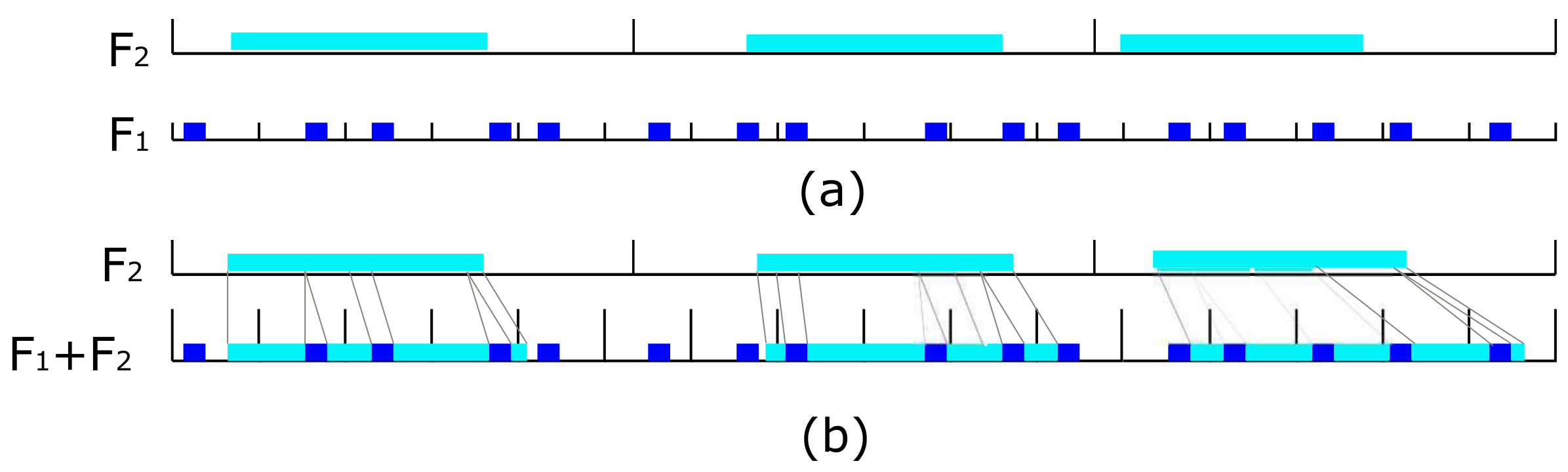
As depicted in Figure 2a, represents a large flow and a small flow. When they are sent to the same link, will occupy multiple periods of . Similar to task scheduling, it is easy to think of assigning different priorities to different flows, and then a higher priority flow can preempt lower ones. Figure 2b indicates the scheduling effect after is preempted by based on the traditional scheduling algorithm, RMS, EDF, or LLF. is divided into three segments, but the cutoff positions, the number, and the size of the segments are unpredictable. Apart from this, these algorithms have the following features. An RMS algorithm flow with a smaller period has higher priority and can provide a stable scheduling strategy while the utilization is limited to about 70%. An EDF (LLF) algorithm flow with the earliest deadline (least slack) has higher priority and has a utilization close to 100%, although the priority is unstable.
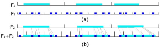
Figure 2.
Large and small flow co-exist scenario (a) two independent periodic flow, is bigger than multiple . (b) is preempted by several times, the cutoff positions are unpredictable.
Generally, we hope the initial offset in the first period of each flow will repeat in the following periods like TTE; however, because preemption is inevitable and unpredictable, the delay and jitter of the preempted parts will be out of control. Therefore, we propose flow-based deterministic scheduling (FDS). Just as TTE knows the location and length of all the frames in every period, FDS considers the offset of each flow and the time when preemption happens in every period. Then, we can schedule the flow but not the frame to support large traffic and meanwhile calculate the detailed information on the frame level. It is stable and has about 100% utilization. Table 1 shows the comparison.

Table 1.
Different scheduling strategy comparation.
Assume the flow set and are given. These flows will repeat in a hyperperiod, , which is the least common multiple (lcm) of all the periods in the flow set. If is not cut off by other flows, we need to know all the offsets, , …, , in its hyperperiod, . If is preempted, we can set , where and is the j-th segment, which has the offsets, , …, , and transmission time, , …, in . According to the above analysis, determines the number of variables and the size of the problem. When , FDS is basked to one flow per period scenario, it is very similar to one frame per period of TTE. So the key problem is to find proper .
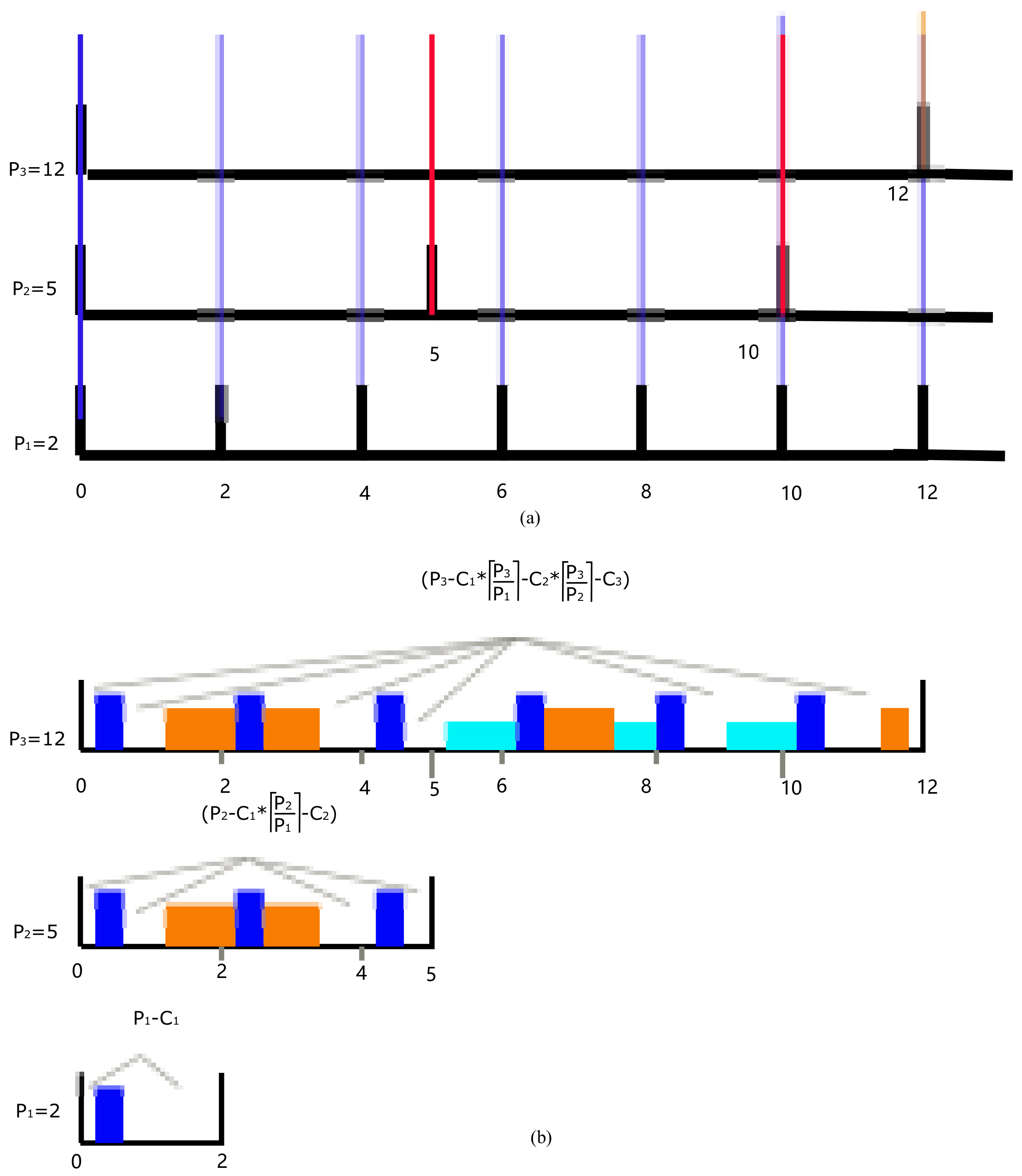
Firstly, we consider two flow scenarios illustrated in Figure 3; the two flows are zero-released, , , and , , , respectively. Assume is atomic and its periodic flow can move back and forth within its period; the maximal available transmission time is and the minimal is 0 as shown in Figure 3a. is split into segments, which is the lower bound of . If has no jitter and is set as anchoring flow, the periodic flow of comes out in fixed time in every period. Figure 3b shows that is split into segments, which is the upper bound of . However, these two extreme cases indicate is changing and hard to be predicted. If we slightly adjust the offset of as shown in Figure 3c, bringing in jitter, the segments of can keep the same number and size as a previous period in . Therefore, it can be the first rule of . To further simplify the number of parameters, we specify previous segments that have the same size, , and the size of the last segment is . In this way, a segment set of flow can be represented as and we have
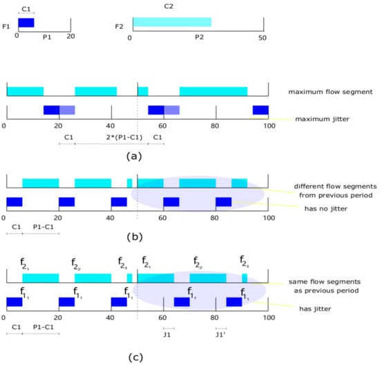
Figure 3.
(a) The maximum segment of when reach maximal jitter. (b) The minimal value of when has no jitter. (c) is preempted by 2 times at the same cutoff positions, it is predictable.
After considering the two flow scenarios, Equation (1) is also suitable for multiple flows. Namely, , we have waiting for scheduling. Before obtaining , we need to compute the available transmission time for multiple periodic flows. We have the following theory.
3.1. Available Transmission Time Theory
Definition 6 (available transmission time).
The accumulated time that can be used for transmitting certain flows when all the flows are considered in the same timeline.
Theorem 1.
Given a set of periodic flows, , the available transmission time for is
We use an inductive approach to give a strict proof.
Proof.
It is very clear that if , then , which means the whole interval in period is available for .
If , then , which means the available for is minus the occupied interval for times.
Assume that for an arbitrary , is true, i.e., . Let us derive from this assumption. For , the available interval in will repeat times and will consume the available interval times. Then the left time for is .
Bringing in the expression, we have
It can be directly obtained that if is divisible by and is divisible by , , …, . Otherwise, we need to consider the essence of the expression. We can see is an estimate of the number of occurrences of in period and is an estimate of the number of repetitions of in period . The product of the two values is computed from the number of final repetitions of in ; therefore, we can replace with . It can minimize the loss of data rounding. In the same way, should be . Then, we can see that (1) holds when . Above all, the claim follows. □
According to the theorem, we have the following corollary about the utilization of FDS.
Corollary 1.
The FDS scheduling utilization can close to 1.
Proof.
According to Theorem 1, if all the available transmission time is exhausted, namely , then the whole transmission time is used by flows, , and we have . After dividing on side, we can obtain . Using the same way as the proof of theorem 1, we can eliminate and obtain the approximate sum of the occupied ratio of , which is the utilization that is close to 1. Then, the corollary claims. □
We can easily have the following corollary about schedulability without proof.
Corollary 2.
The flow can be schedulable if only if
The corollary means the total occupied time in period should be less than the available interval. It can be used to judge whether a new flow can be added. If the available interval is enough, it is important to arrange related flow in such an interval. As depicted in Figure 4, if , must be preempted. Next, we need to estimate the number of segments .
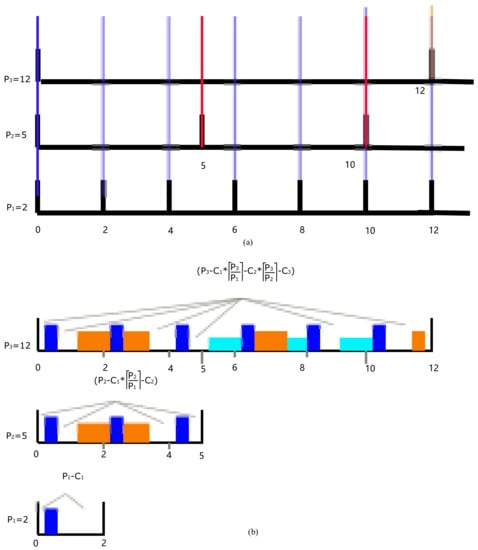
Figure 4.
(a) The possible blanks that split by small period. (b) Example for the available transmission time in one period after the flow has been scheduled.
3.2. Segment Estimation
If all the periods are zero-released and we align smaller , where in the interval . Algorithm 1 presents a simple way to compute the number of blocks that a smaller period cut a larger period. For example, in Figure 4, , , , can split into three blocks, and can together split into seven blocks. In our model, these estimated values are treated as a reference. Then, we have to obtain the estimated average available space in each block for flow by
where is the number of split blocks in one period . The core idea is to repeat all periods in the hyperperiod and sort them in ascending order. The first index of value is . The estimated can be
If there is , flow has to preempt at least times, which can be used as reasonable evidence of our estimation algorithm.
| Algorithm 1 Estimated number of segment |
|
4. Constraints Formulation
After obtaining , the components of the scheduling flow set are also determined. The objective is to compute the offsets of all the flows and then transfer them into the gate control list. We use SMT to build the following first-order constraints. It mainly includes intra and inter-flow and task constraints in computing nodes.
4.1. Intra Flow Constraint
4.1.1. Boundary Constraints
The segment of flows needs to satisfy the boundary constraints, which means all the segments need to stay at their period. and are the first and the last segments, respectively, in its -th period. The other segment needs to keep transmission order in the same period. Unlike the constraints in the literature [18,19,20], the constraint of each segment in each period is independent of other periods in the same flow hyperperiod.
The number of constraint inequalities is about , where denotes the size of the set.
4.1.2. Dispersion Degree Constraints
Since the segment may be dispersed in all the possible positions in the period if it only satisfies the boundary constraint. The time span between and might cover the whole period, even if the is small. Hence, we introduce a coefficient , called the dispersion degree, to adjust the time span. We have the dispersion degree constraints.
The number of constraint inequalities is about . In this constraint, to keep the same scaling ratio, we use the same for one flow. It can further guarantee its stability at the task level. This constraint can improve performance when the whole system has a solution. It is usually used as an additional supplementary based on boundary constraints.
4.1.3. Local Jitter Constraints
As the segment from the different periods might have different offsets, it will bring inter-period jitter in the same flow period. By taking the segment in the chosen period as a reference, we set local jitter constraints.
The number of constraint inequalities is about . Usually, the first period is the chosen one, and the difference between the period and all the other corresponding segments in the subsequent periods is limited to . It is also supplementarily based on the boundary constraints. If , the offset of all the segments in each period is equal to each other, then the model can be simplified by only considering the first period like the TTE model. This strict constraint will reduce the solution space and bandwidth utilization. When and , we can obtain the maximal , namely , where the constraints has no practical effect. Hence, by adjusting , we can control the trade-off between bandwidth utilization and jitter.
4.1.4. Hop Latency and Jitter Constraints
The previous constraints focus on single-node scenarios. Next, we consider the constraints when the flows are transmitted from one node to its adjacent node. To make sure the scheduling can succeed, the difference between the corresponding segment should be larger than the possible maximal hop delay so that the switch can successfully finish the switching operation. Because the time synchronization based on 802.1 Qas still introduces the synchronization time jitter , we add this value to tolerate the possible fluctuation.
These constraints are for flow schedulable of the flow set on path . The number of constraint inequalities is about .
4.1.5. End-to-End Latency and Jitter Constraints
At the level of the task, it has a latency requirement. The tik starts with sending the first bit and the tok ends with receiving the last bit. The whole time to finish flow in each period, , should be less than the end-to-end latency . Meanwhile, the end-to-end jitter should also keep at a proper value. Unlike the local jitter control, it is hard to find a reference, so we bound the difference between maximal and minimal latency by a .
The number of constraint inequalities is about .
4.2. Inter Flow Constraint
Besides the intra flow constraints, the several co-existing flows in the same node might contend the same output link. When these flows interleave together, we need the following constraints to minimize the influence of each other.
4.2.1. Contention Free Constraint
Unlike the previous literature [18,21,22], we only handle the overlapping parts from different flows in its hyperperiod. It can effectively minimize the number of constraints.
The number of constraint inequalities is about or . Similarly, harmonious periodic flows can reduce the constraints.
4.2.2. Link Bandwidth Constraint
If multiple flows share the same link, the whole bandwidth consumption has its boundary. According to Corollary 1, the sum of the occupied ratio of all the flows should satisfy the bandwidth constraint on every link.
The number of constraint inequalities is about .
4.3. Task Constraint
4.3.1. Computing Capability Contraint
All the tasks should satisfy the computing capability constraint. Let U denote the utilization function; then, we have
Task scheduling has many mature solutions, to which we will not go into much detail here. The number of constraint inequalities is about .
4.3.2. Task Contention Free Constraint
In one node, the task scheduling should avoid contention like the interflow contention free.
4.3.3. End-to-End Task Delay Constraint
To guarantee deterministic holistic scheduling, end-to-end scheduling is critical. Except for the contention of the computing resource, it is important to align the task with the flow in a timeline. The tasks that need end-to-end scheduling should satisfy the end-to-end delay and jitter requirements.
The constraints indicate that task must finish execution before it releases the flow in the sender. Meanwhile, the receiver should start executing the task after the transmission of is finished. The number of constraint inequalities is about .
5. Independently Programmable Flow Subset
As our model is end-to-end scheduling and some flows are split into subsegments, the set of flows on one link will change when transmitted from one hop to the next hop. Some sets of flows are separated because they are switched into different ports, and some are converged from different ports into the same port. It is not practical to plan all the flows in the entire network for all the cases; we propose independent programmable flow subsets to minimize the number of variables in each independent scheduling.
Definition 7 (Independent programmable flow (IPF) subset).
The minimal flow set that can independently make flow segmentation.
Consider the abstract graph of Figure 1. Table 2 presents all the flows in the same direction sharing the same output port and link. The transmission paths and their related flows are presented in Table 3. Take as an example; link has , , , has , and has , . Assume the output port of the source nodes are the start-point where flows might be split into segments. All the flows should be considered in advance so that there is enough space to be allocated for all the flows. Hence, needs to consider the cover set of the flows on all its links, namely flow set . Meanwhile, needs to consider flow set . Then, we find and are connected because of . Flows and are both needed to be considered by . In this way, all the paths are connected by the intersecting flows, and then all the flows should be considered together. In this example, the IPF subset includes all the flows in the topology. The example shows that there are still relationships, even if some flows have completely different paths.
Table 2.
The flows on the directed link.
Table 3.
The flow sets on all the paths.
Generally, the connections built up by the intersecting flows are universal in such a multiple-node system, even if the flows are not split. One extreme case is that when all the flows have different prime periods the whole connected flows must be considered entirely to allocate the resource. Fortunately, the practical network usually adopts harmonic periods and constructs disjoint and redundancy paths, such as IEC 61508. The harmonic period means a small hyper-period and the flow set on one disjoint path can be treated as the IPF subset. Furthermore, the same period flows might cut off the connections when they have a similar size. For example, if flows and have the same period and similar size, namely the estimated number of segment for each flow, , and have no change and , then flow set or can be considered independently. Therefore, we propose the following algorithm to find the IPF set.
The goal of Algorithm 2 is to find the maximum number of period flows that can be independently programmed. From line 1 to 10, it records all the flows that will be transmitted on each link after initializing the flow–link matrix with false. Then, we unite all the flows on each link on a certain path from line 11 to 15. In this step, there would be real flow on the corresponding link. After scanning all the paths from line 16 to 23, we can obtain all the possible IPF subsets. Finally, we can compare all the possible IPF and categorize them into different IPF subsets from line 24 to 26.
| Algorithm 2 Independent programmable flow subset |
|
After identifying IPS, we use a segment estimation algorithm to compute the parameters of the flow or split-flow and then construct the constraint models based on formulations in Section 4. We can obtain the offsets of all the flows and tasks. If there is no split, each task has a list of offsets within its own hyper-period on the sender side, and the corresponding flow has delayed offsets in each TSN node. Because different flows may converge on a node and one of the flow’s offset plus its duration equals to other’s offset, we need to merge the offsets to find the start-time and end-time of the last GCL. If the flow is split, each task still keep one sending offset per period hyper-period, while the corresponding flow will be cut into several sub-flows and each sub-flow has its own offset. The sub-flows will be treated as normal flow to participate in the final merger into GCL.
6. Experiment and Evaluation
6.1. Experiment Setup
Based on the previous analysis, we implemented a simulation for a schedule, where we formulated the first-order logical constraint using the SMT model and solved by Z3 [23] v4.8.8-64bit, which runs on an Intel(R) Core(TM) i7-8700 64bit CPU @ 3.20 GHZ with 16 GB of RAM.
Assume the network bandwidth is 1 Gbps, and the minimum and maximum frame sizes are 84 and 1542 bytes according to IEEE 802.1 Q. The transmission time is 0.672 μs and 12.336 μs, respectively. Meanwhile, 84 bytes can also be treated as the shortest preempted frame according to IEEE 802.1 Qbu. For the IFS (inter-frame space) and the convenience of calculation, we round the two values as 1 unit and unit, where 1 unit ≈ 0.672 μs. We classify all the flows into three types.
- Ant flow, one frame per period, when transmission time varies within the range ;
- Mice flow, up to 10∼100 MTU frames per period, when transmission time varies within the range
- Elephant flow, more than 100 MTU frames per period, when transmission time varies within the range in , where X is its maximum period.
Each type has a matching period. In TTE and Flexray, the size of macrotick is about 60 μs to 1 ms, and the frame size is about 500 Bytes. So we refer to macrotick and set the period boundary for ant flows as , which is a finer time precision than that of TTE and Flexray. Then, we set [1001, 10,000], [10,001, 50,000]. Here, taking 50,000 unit ≈ 33 ms as the supper boundary for elephant flow is based on the requirement of 720P-30FPS (720P video at 30 FPS (frames per second) without compression, which needs about 2.8 MB per 30 ms to be transmitted, close to 1850 MTU frames per 33 ms).
Since there is a total of eight queues per port, we assume one queue for deadline-constrained aperiodic flows, one for BE flows, and two queues for 802.1 QCF. Four queues can be used for periodic flows. More radically, we map one period to one queue and one flow per period. The above constraints indicate that hyper-period takes a major proportion of the number of constraint inequalities, so we take the harmony period in the experiment.
6.2. Offset Computation Evaluation
Firstly, we consider the offset computation evaluation, where different groups of multiple periodic flows are depicted in Table 4.
Table 4.
Flow parameters.
For any flow, we only take one value for flow size due to its small range of variation, while we take three periods because the change has an impact on the available interval and then on the number of segments for elephant flow. For mice flow, we take three kinds of periods and three kinds of flow sizes. For elephant flow, six kinds of flow sizes are taken for the large range of variation and we only take two kinds of period which will be used by matching the flow size. We need to choose four flows to verify that flow-level programming has less constraint in contrast to frame-level programming. If there are too many combinations to experiment, we adopt a partial-flit way to observe the change in the number of segments in Table 5.
Table 5.
Partial-flit to observe the change in the number of segments vs. the number of frames.
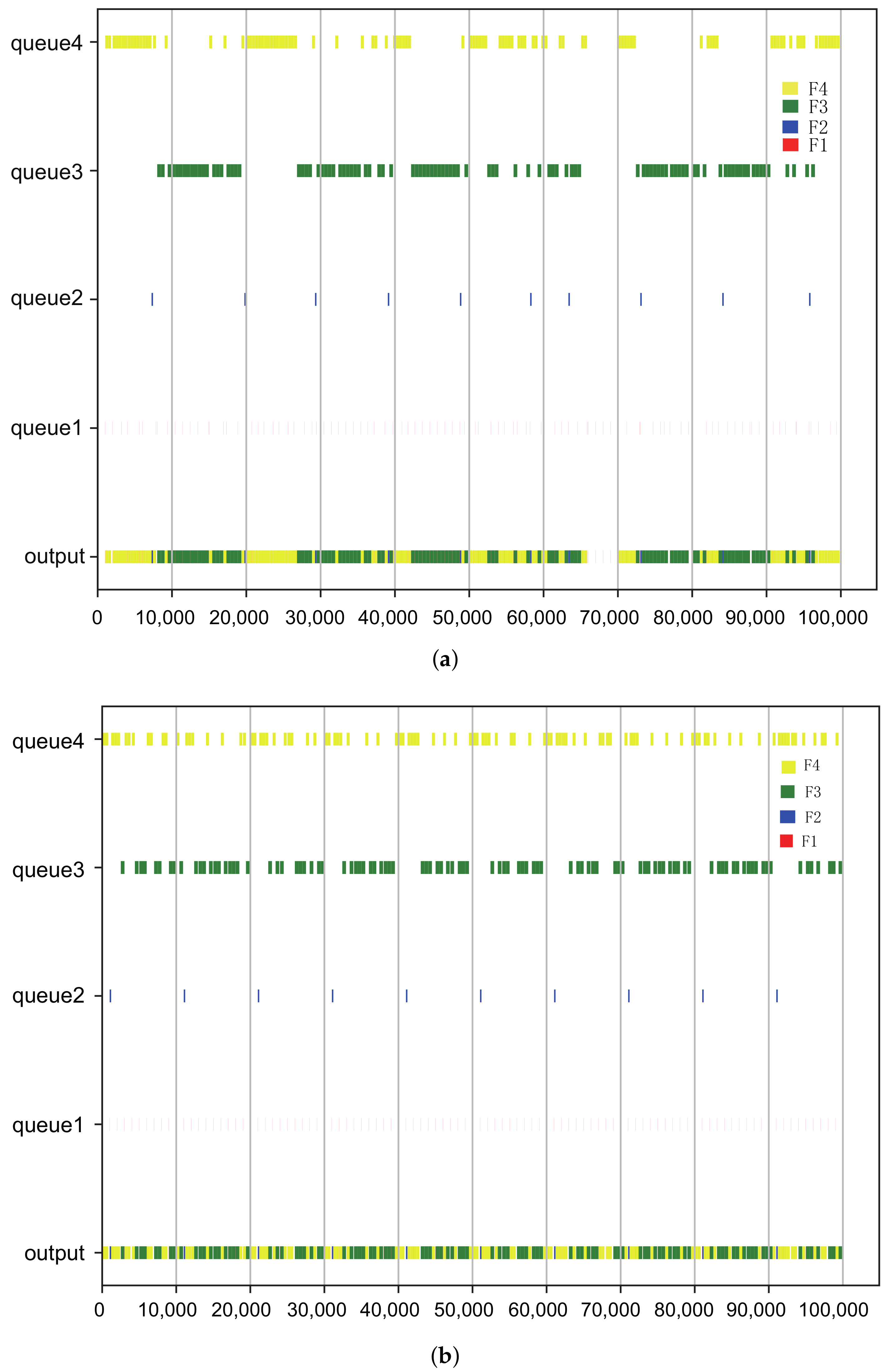
For example, there are only one or two flows incrementally changed from to . As can be seen from the table, the number of frames keeps increasing with the growth of flow size and utilization, while flow-level strategy can reduce the number of scheduling variables, which means it can largely shorten the synthesis time. One direct programming result of is illustrated in Figure 5. In Figure 5a, only the boundary and contention-free constraints are used, we can see the large flow has been split into many segments and major of them are larger than a single frame. Based on the two kinds of constraints, Figure 5b depicted the effect when the intra-flow jitter constraint is imported. The jitter of queue1 and queue2 has improved.
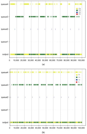
Figure 5.
Gantt chart for scheduling. (a) Boundary and contention-free constraints. (b) Add an intra-jitter constraint to (a). Different colors mean the corresponding gate for the flows F1, F2, F3 and F4 in shown in Table 5.
After the problem of multiple flows in single-port has been solved, we try to consider the end-to-end scheduling problem. Here, we consider the model in Figure 1; there are six tasks whose periods are chosen based on Table 4 and make sure they have chosen different periods. Then, every task randomly chooses the flow size related to its period. The six flows are treated as their generated task. The task shares the same period as its flow, while their WCET is set as a random value between 1 and 50. The hop-delay of switches is determined by their flow size, if the flow size is less than MTU, then the maximum hop delay is the flow size; otherwise, the value of MTU is 20. After this setting, we can build a first-order constraint to reach end-to-end schedulability. Our goal is to minimize the end-to-end delay. Firstly, at some time, all the periodic flow will be put together to obtain the way to split. Then, each segment needs to satisfy hop-to-hop constraints. We evaluate the synthesis time of the following task set.
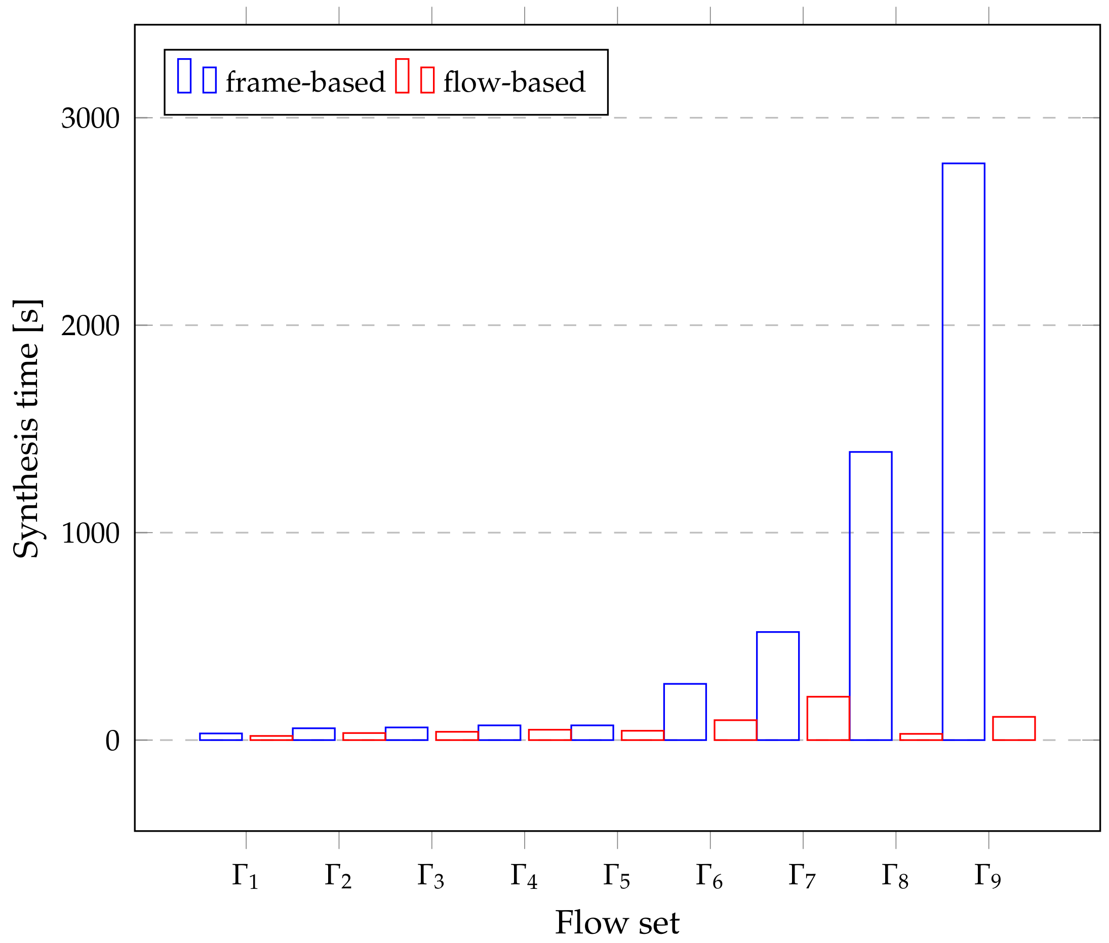
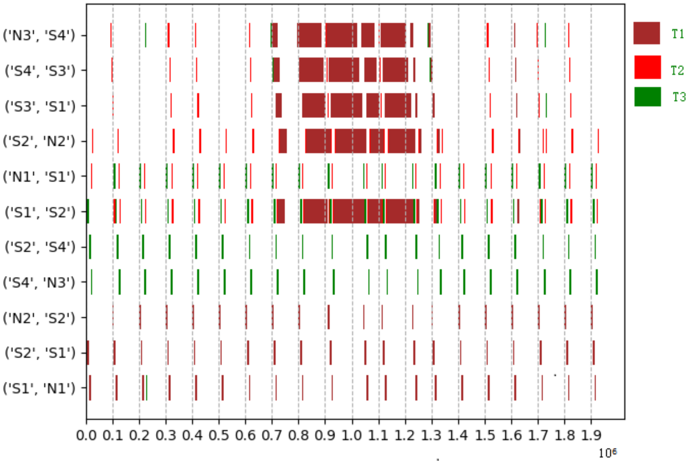
Compared to frame-based scheduling, Figure 6 represents the number of variables needed to construct the constraint solution, and Figure 7 shows the preliminary synthesis time of the task set in Table 5. Since tasks and flows can be treated as the same coarse-grained entity, the mapping relationship from tasks to flows or segments is easy to express, especially for tasks that require large traffic. Therefore, it is easy to handle the temporal logic between the network and tasks in the holistic schedulable scenario, resulting in a significant drop in synthesis time. The time series Gantt chart in Figure 8 shows all the scheduled time for all the tasks, flows or sub-flows that can be tracked in each link. As can be seen from the figure, large flows can be elegantly split and separated without harming smaller flows.
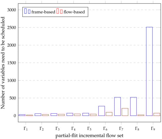
Figure 6.
Number of variables need to be scheduled based on frame vs. flow.
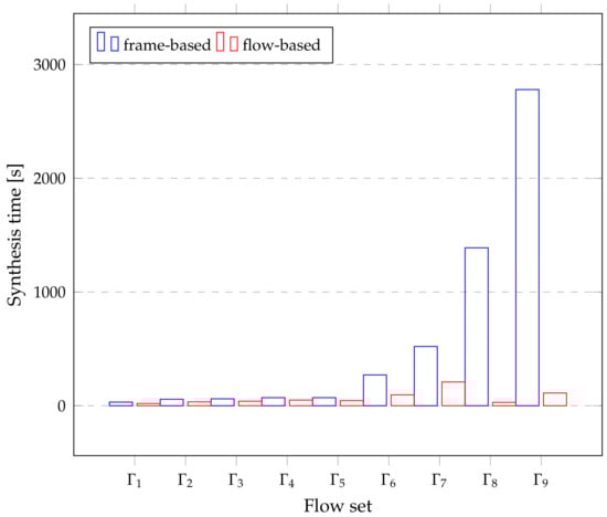
Figure 7.
The synthesis time of holistic scheduling based on frame or flow.
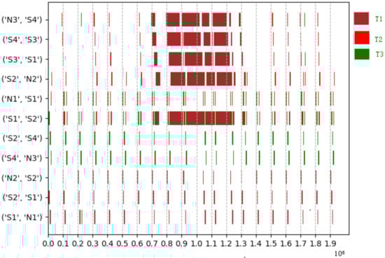
Figure 8.
The scheduling time for in Table 6 on each link after GCL is active. The links starting with ’N1, N2, N3’ depict the sending time offsets for task. Different color gates represent the different tasks.
6.3. Various Topology with Multiple Periods
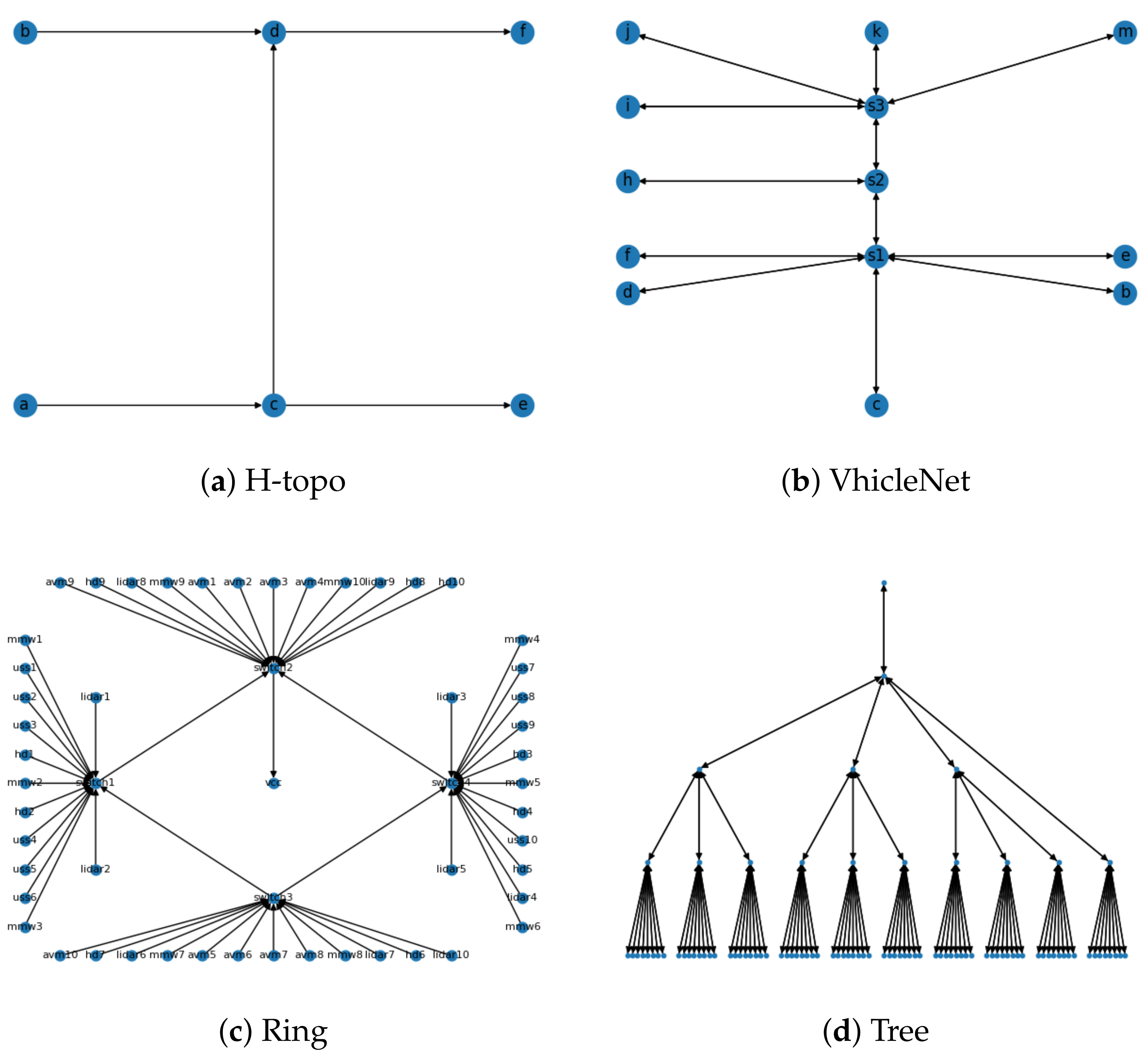
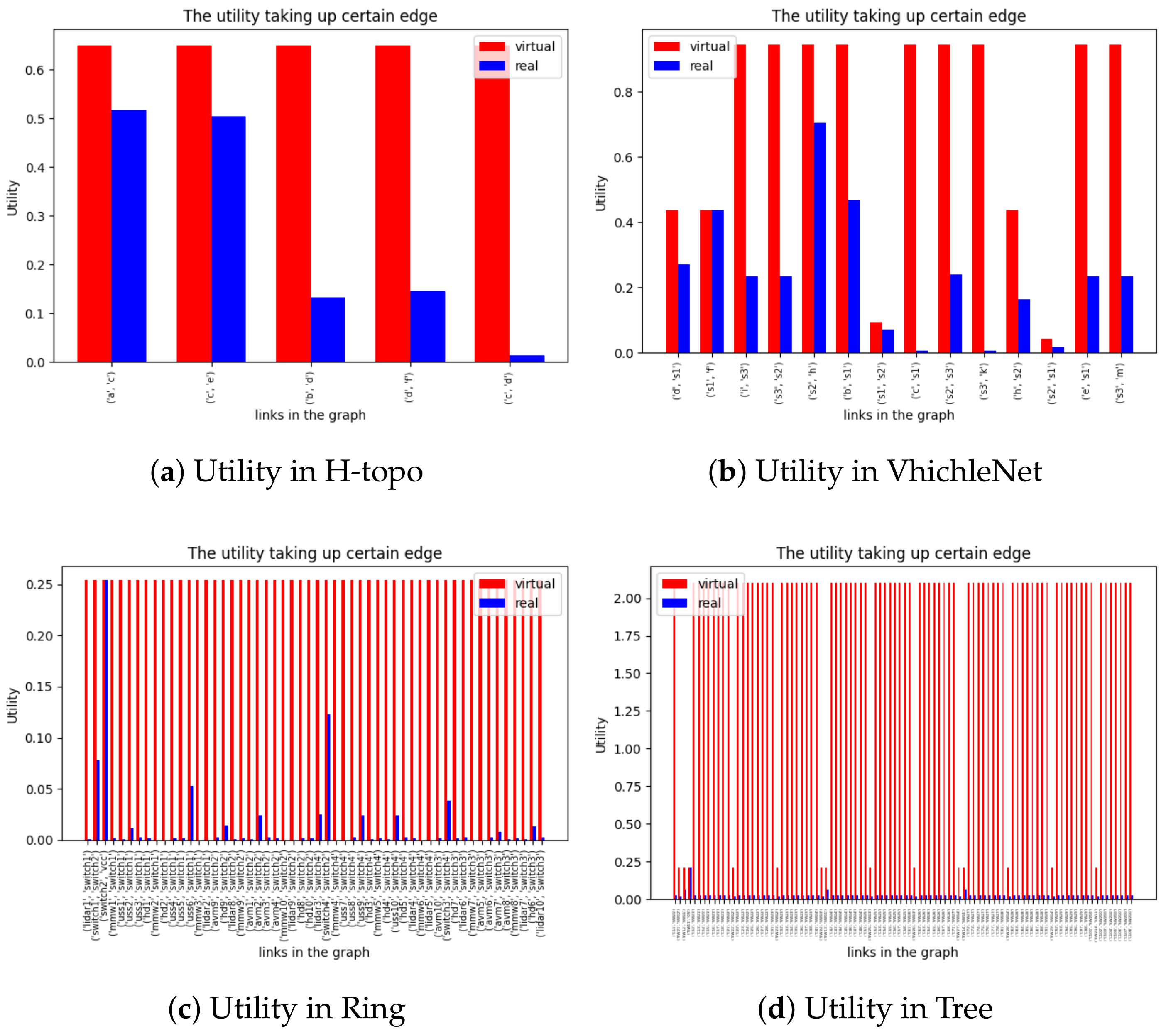
To verify the generality of the model, we constructed four representative network topologies and task models for experiments, and focused on the schedulability of the model in the experiments in Figure 9. Due to excessive SMT constraints, we can only obtain the offset time of flows or tasks when there are feasible solutions. In this model, single-node scheduling pursues utilization by splitting large flows, but due to changes in topology, we need to solve an IPF, which reduces the overall solution space. Figure 10 compares the feasible solutions obtained after approximately 20 rounds, and due to the existence of IPF, there is a real and virtual traffic occupancy on each link. Due to the differences in period and path, in order to ensure constraints such as end-to-end, the virtual flow can be interpreted as the interval time that must exist when the flow is scheduled on different links. During the actual trial period, the space occupied by these virtual traffic can be allocated to BE traffic. As can be seen from Figure 10a–d, as the network becomes increasingly complex, its true bandwidth utilization also decreases to some extent. This is due to the fact that the use of IPF results in a sharp decrease in the solution space due to the correlation between links and flows. This is also some of the shortcomings of the model, which we will optimize in our future work
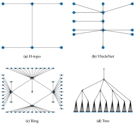
Figure 9.
Network topology in the simulations.
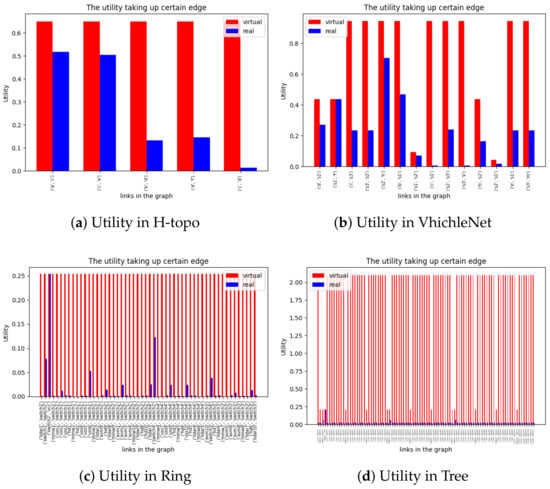
Figure 10.
The bandwidth utilizaion for different topologies using our model.
7. Related Work
Steiner [19] defined SMT-base evaluation for TTE in multihop networks. It focused on building one-frame-per-period constraints and precisely formulating the scheduling problem. Many of the constraints provide a good reference for us to build our work. As mentioned in the previous section, it can be our special case when we only consider the network part. After that, Oliver et al. [2,24] and considered building a similar constraint by obeying the standard itself of IEEE 802.1 Qbv. It extends a single frame in TTE to multiple frames and the scale of the problem grows extremely, making it hard to resolve. Meanwhile, they also combined the task and network based on TTE [13] to make a schedule, and they pointed out that the number of frames is the biggest bottleneck to expanding the scale. Furthermore, when considering the coordination between routing and scheduling [25], the problem becomes complex and difficult to solve due to the sharp increase in the number of variables. Our flow-level scheduling might be an option to break the bottleneck for it can reduce the number of variables for these models. Ref. [18] adopted the first-order theory of arrays to express constraints and exposed synthesis of schedules via an SMT solver. It assumes the message size of one Ethernet frame and constructs time windows for GCLs based on IEEE 802.1 Qbv. In this model, the scale of the whole synthesis is still limited to 1000 frames of magnitude; the experiment shows that it takes 40 h to synthesize 264 frames with 32 windows. It is unacceptable in our megabytes per period scenarios. TSNsched [26] is a tool for generating TSN schedulers. They consider the flow fragment in their constraint and claim TSNshed can support both individual packets and time windows; however, how to generate such fragment is still unknown. In their experiment, the flow size is limited to five frames and there is no evaluation of utilization. Concerning these works, we discuss the method of generating segments, called fragments in [26] and the time window in [18]. Even though time windows have been introduced into industrial applications [27], the mapping problem from the frame to the window still exists. We think our work can make up the gap between frame and flow.
8. Conclusions
The conventional approach, inspired by the Internet, is to decouple task and network scheduling, while TSN strives to provide deterministic data streams and the computing nodes adjust their processing logic based on the parameters that the network can provide.
In this paper, we propose a joint programming method for real-time task and network scheduling. By considering periodic task execution and end-to-end network transmission together, we construct first-order constraints for an SMT (satisfy module theory) problem. Unlike related work, our method can achieve near 100% bandwidth utilization on a single TSN node. Moreover, it can reduce the number of constraints based on flow-level scheduling. FDS differs from the existing task and joint scheduling strategies in that it can elevate the scheduling granularity of TSN data transmission from the frame level to the flow level, which can establish a one-to-one correspondence between the time control granularity at the task level and the granularity of network transmission, and has potential cross-layer transmission capabilities.
Author Contributions
Conceptualization, Y.C., H.Z. (Huayu Zhang) H.Z. (Hailong Zhu) and H.Z. (Haotian Zhan); methodology, Y.C., H.Z. (Huayu Zhang), H.Z. (Hailong Zhu) and H.Z. (Haotian Zhan); software, Y.C., H.Z. (Huayu Zhang), H.Z. (Haotian Zhang), N.C., H.Z. (Hailong Zhu), P.Z. and H.Z. (Haotian Zhan); validation, Y.C.,H.Z. (Huayu Zhang), H.Z. (Haotian Zhang), Y.L., N.C., Z.Z., H.Z. (Hailong Zhu), P.Z. and H.Z. (Haotian Zhan); investigation, Y.C.,H.Z. (Huayu Zhang), H.Z. (Hailong Zhu) and H.Z. (Haotian Zhan); data curation, Y.C., H.Z. (Huayu Zhang), H.Z. (Hailong Zhu) and H.Z. (Haotian Zhan); writing—original draft preparation, Y.C., H.Z. (Huayu Zhang), H.Z. (Haotian Zhang), N.C., H.Z. (Hailong Zhu), P.Z. and H.Z. (Haotian Zhan); writing—review and editing, Y.C., H.Z. (Huayu Zhang), H.Z. (Haotian Zhang), N.C., H.Z. (Huayu Zhang), P.Z. and H.Z. (Haotian Zhan); visualization, Y.C., H.Z. (Huayu Zhang),H.Z. (Haotian Zhang), N.C., H.Z. (Hailong Zhu), P.Z. and H.Z. (Haotian Zhan); supervision, Y.C., H.Z. (Huayu Zhang), H.Z. (Haotian Zhang), Y.L., N.C., Z.Z., H.Z. (Hailong Zhu), P.Z. and H.Z. (Haotian Zhan); project administration, Y.C., H.Z. (Huayu Zhang), H.Z. (Haotian Zhang), Y.L., N.C., Z.Z., H.Z. (Hailong Zhu), P.Z. and H.Z. (Haotian Zhan); All authors have read and agreed to the published version of the manuscript.
Funding
This work is partially supported by the Scientific Research Programs for High-Level Talents of Beijing Smart-chip Microelectronics Technology Co., Ltd., and partially supported by the Academician Expert Open Fund of Beijing Smart-chip Microelectronics Technology Company Ltd., and partially supported by the Natural Science Foundation of Shandong Province under Grant ZR2022LZH015, and partially supported by the Key Funding from National Natural Science Foundation of China under Grant 92067206.
Data Availability Statement
The data presented in this study are available on request from the corresponding author. The data are not publicly available due to privacy.
Conflicts of Interest
The authors declare no conflict of interest.
Abbreviations
| Set of live tasks at time t | |
| Number of tasks in | |
| when is constant in a long term | |
| Start time of task | |
| End time of task | |
| Set of periodic tasks | |
| Set of deadline-constraint aperiodic tasks | |
| Tuple representing offset in each period, WCET, deadline and period for periodic tasks | |
| Deadline for deadline-constraint aperiodic task | |
| The task set on node , containing local tasks, input tasks, and output tasks. | |
| Local tasks on node . | |
| Input tasks to node . | |
| Output tasks from node . | |
| The flow from node to node . | |
| The flow set on node . | |
| A bijective relationship between tasks and flows. | |
| The flow set on node corresponding to its output tasks. | |
| The flow corresponding to a specific task. | |
| Offset in each period, transmission time, deadline, and period of a flow. | |
| Transmission time of a flow. | |
| Deadline and period of a flow are the same as its corresponding task deadline and period, usually. | |
| The flow set on link . | |
| The flow on link . | |
| The period of flow . | |
| The transmission time of flow . | |
| The set of destination nodes that node will send data flow to. | |
| The set of source nodes that node will receive data flow from. |
References
- Akella, A.; Seshan, S.; Karp, R.; Shenker, S.; Papadimitriou, C. Selfish behavior and stability of the internet: A game-theoretic analysis of TCP. In Proceedings of the 2002 Conference on Applications, Technologies, Architectures, and Protocols for Computer Communications (SIGCOMM’02), New York, NY, USA, 19–23 August 2002. [Google Scholar]
- Craciunas, S.S.; Oliver, R.S.; Chmelik, M.; Steiner, W. Scheduling real-time communication in IEEE 802.1 Qbv Time Sensitive Networks. In Proceedings of the 24th International Conference on RealTime Networks and Systems (RTNS), Brest, France, 19–21 October 2016. [Google Scholar]
- Nasrallah, A.; Thyagaturu, A.S.; Alharbi, Z.; Wang, C.; Shao, X.; Reisslein, M.; Elbakoury, H. Performance Comparison of IEEE 802.1 TSN Time Aware Shaper (TAS) and Asynchronous Traffic Shaper (ATS). IEEE Access 2019, 7, 44165–44181. [Google Scholar] [CrossRef]
- Jin, X.; Xia, C.; Guan, N.; Xu, C.; Li, D.; Yin, Y.; Zeng, P. Real-Time Scheduling of Massive Data in Time Sensitive Networks with a Limited Number of Schedule Entries. IEEE Access 2020, 8, 6751–6767. [Google Scholar] [CrossRef]
- CAN Specification; Robert Bosch GmbH: Stuttgart, Germany, 1991.
- Makowitz, R.; Temple, C. FlexRay—A communication network for automotive control systems. In Proceedings of the IEEE International Workshop on Factory Communication Systems, Turin, Italy, 28–30 June 2006; pp. 207–212. [Google Scholar]
- LIN Specification Package, Revision 2.0; LIN Consortium: Dallas, TX, USA, 2003.
- Kopetz, H.; Ademaj, A.; Grillinger, P.; Steinhammer, K. The time-triggered ethernet (tte) design. In Proceedings of the Eighth IEEE International Symposium on Object-Oriented Real-Time Distributed Computing (ISORC’05), Seattle, WA, USA, 18–20 May 2005; pp. 22–33. [Google Scholar]
- Craciunas, S.S.; Oliver, R.S. An Overview of Scheduling Mechanisms for Time-sensitive Networks. In Proceedings of the 8th International Workshop on Analysis Tools and Methodologies for Embedded and Real-time Systems (WATERS 2017), Dubrovnik, Croatia, 27 June 2017. [Google Scholar]
- Lehoczky, J.; Sha, L.; Ding, Y. The rate monotonic scheduling algorithm: Exact characterization and average case behavior. In Proceedings of the Real-Time Systems Symposium, Santa Monica, CA, USA, 5–7 December 1989; pp. 166–171. [Google Scholar]
- Lehoczky, J.P.; Ramos-Thuel, S. An optimal algorithm for scheduling soft-aperiodic tasks in fixed-priority preemptive systems. In Proceedings of the Real-Time Systems Symposium, Phoenix, AZ, USA, 2–4 December 1992. [Google Scholar]
- Sha, L.; Abdelzaher, T.; Årzén, K.E.; Cervin, A.; Baker, T.; Burns, A.; Buttazzo, G.; Caccamo, M.; Lehoczky, J.; Mok, A.K. Real Time Scheduling Theory: A Historical Perspective. Real Time Syst. 2004, 28, 101–155. [Google Scholar] [CrossRef]
- Craciunas, S.S.; Oliver, R.S. Combined task and network-level scheduling for distributed time-triggered systems. Real-Time Syst. 2016, 52, 161–200. [Google Scholar] [CrossRef]
- Feng, T.; Yang, H. SMT-based Task and Network level Static Schedule for Time Sensitive Network. In Proceedings of the IEEE International Conference on Communications, Information System and Computer Engineering (CISCE), Beijing, China, 14–16 May 2021. [Google Scholar]
- Li, Y.; Li, Z.; Wu, J. Task scheduling and network traffic control for time-sensitive networks. J. Comput. Sci. Technol. 2020, 35, 249–265. [Google Scholar]
- Zhang, Y.; Wang, C.; Liu, J. Joint task scheduling and flow control for time-sensitive networks. IEEE Trans. Parallel Distrib. Syst. 2019, 30, 1218–1231. [Google Scholar]
- Liu, B.; Chen, Y. A survey on task scheduling and network flow control for time-sensitive networks. J. Comput. Sci. Technol. 2018, 33, 949–964. [Google Scholar]
- Oliver, R.S.; Craciunas, S.S.; Steiner, W. IEEE 802.1 Qbv Gate Control List Synthesis using Array Theory Encoding. In Proceedings of the IEEE Real-Time and Embedded Technology and Applications Symposium (RTAS), Porto, Portugal, 11–13 April 2018. [Google Scholar]
- Steiner, W. An evaluation of smt-based schedule synthesis for time triggered multi-hop networks. In Proceedings of the 2010 31st IEEE Real-Time Systems Symposium, San Diego, CA, USA, 30 November–3 December 2010; pp. 375–384. [Google Scholar]
- Pozo, F.; Steiner, W.; Rodriguez-Navas, G.; Hansson, H. A decomposition approach for smt-based schedule synthesis for time-triggered networks. In Proceedings of the 2015 IEEE 20th Conference on Emerging Technologies & Factory Automation (ETFA), Luxembourg, 8–11 September 2015; pp. 1–8. [Google Scholar]
- Sha, L.; Abdelzaher, T.; Årzén, K.E.; Cervin, A.; Baker, T.; Burns, A.; Buttazzo, G.; Caccamo, M.; Lehoczky, J.; Mok, A.K. Reducing the Number of Preemptions in Real-Time Systems Scheduling by CPU Frequency Scaling. In Proceedings of the International Conference on Real-Time & Network Systems, Toulouse, France, 25–27 November 2010. [Google Scholar]
- Dürr, F.; Nayak, N.G. No-wait packet scheduling for IEEE time-sensitive networks (TSN). In Proceedings of the 24th International Conference on Real-Time Networks and Systems (RTNS), Brest, France, 19–21October 2016; pp. 203–212. [Google Scholar]
- Moura, L.D.; Bjørner, N. Z3: An efficient SMT solver. In Proceedings of the 14th International Conference on Tools and Algorithms for the Construction and Analysis of Systems, Budapest, Hungary, 29 March–6 April 2008; pp. 337–340. [Google Scholar]
- Craciunas, S.S.; Oliver, R.S.; Steiner, W. Formal Scheduling Constraints for Time-Sensitive Networks. arXiv 2017, arXiv:1712.02246. [Google Scholar]
- Atallah, A.A.; Hamad, G.B.; Mohamed, O.A. Routing and Scheduling of Time-Triggered Traffic in Time-Sensitive Networks. IEEE Trans. Ind. Inform. 2020, 16, 4525–4534. [Google Scholar] [CrossRef]
- Dos Santos, A.C.T.; Schneider, B.; Nigam, V. TSNSCHED: Automated Schedule Generation for Time Sensitive Networking. In Proceedings of the 2019 Formal Methods in Computer Aided Design (FMCAD), San Jose, CA, USA, 22–25 October 2019; pp. 69–77. [Google Scholar]
- Reusch, N.; Zhao, L.; Craciunas, S.S.; Pop, P. Window-Based Schedule Synthesis for Industrial IEEE 802.1 Qbv TSN Networks. In Proceedings of the 2020 16th IEEE International Conference on Factory Communication Systems (WFCS), Porto, Portugal, 27–29 April 2020. [Google Scholar]


Disclaimer/Publisher’s Note: The statements, opinions and data contained in all publications are solely those of the individual author(s) and contributor(s) and not of MDPI and/or the editor(s). MDPI and/or the editor(s) disclaim responsibility for any injury to people or property resulting from any ideas, methods, instructions or products referred to in the content. |
© 2023 by the authors. Licensee MDPI, Basel, Switzerland. This article is an open access article distributed under the terms and conditions of the Creative Commons Attribution (CC BY) license (https://creativecommons.org/licenses/by/4.0/).