Article

Enhancing CNNs Performance on Object Recognition Tasks with Gabor Initialization

1
Department of Computer Science, Baylor University, Waco, TX 76798, USA
2
Brazos Innovation Partners, LLC, Waco, TX 76798, USA
*
Author to whom correspondence should be addressed.
Electronics 2023, 12(19), 4072; https://doi.org/10.3390/electronics12194072
Submission received: 31 May 2023 / Revised: 24 September 2023 / Accepted: 24 September 2023 / Published: 28 September 2023
(This article belongs to the Special Issue Convolutional Neural Networks and Vision Applications - Volume III)

Abstract

:
The use of Gabor filters in image processing has been well-established, and these filters are recognized for their exceptional feature extraction capabilities. These filters are usually applied through convolution. While convolutional neural networks (CNNs) are designed to learn optimal filters, little research exists regarding any advantages of initializing CNNs with Gabor filters. In this study, the performance of CNNs initialized with Gabor filters is compared to traditional CNNs with random initialization on six object recognition datasets. The results indicated that the Gabor-initialized CNNs outperformed the traditional CNNs in terms of accuracy, area under the curve, minimum loss, and convergence speed. A statistical analysis was performed to validate the performance of the classifiers, and the results showed that the Gabor classifiers outperformed the baseline classifiers. The findings of this study provide robust evidence in favor of using Gabor-based methods for initializing the receptive fields of CNN architectures.

1. Introduction

Gabor filters have been successfully applied in computer vision for various tasks, such as recognizing objects, textures, and shapes. They have been used in tasks such as invariant object recognition [1], building and road structure detection from satellite images [1], license plate detection [2], traffic sign recognition [3], diagnosis of invasive ductal carcinoma of the breast [4], edge detection [5], texture segmentation [5], image classification [5], fingerprint and face recognition [5], texture recognition [6], and hyperspectral image classification [7]. Gabor filters are known for their ability to extract essential activations, their multi-orientation and multi-scale analysis capabilities, and their effectiveness in texture classification and feature extraction [3,4,7]. They are suitable for texture recognition in computer vision due to their optimal properties in the spatial and frequency domains [3]. Gabor filters have been widely used and have succeeded in various computer vision applications [2,5,7,8,9,10,11,12,13,14,15].
However, in recent years, Vision Transformers (ViTs) [16] and CNNs [17] have overshadowed the use of Gabor filters. CNNs date back to the late 1990s [18] but gained popularity in the early 2010s with the seminal work of Krizhevsky, Stuskever, and Hinton [19]. Since then, numerous model variations have been proposed across various sectors [20,21,22,23,24,25]. Technical limitations previously hindered the widespread use of CNNs, but these limitations have been alleviated with the advent of improved computation power in CPUs, GPUs, TPUs, and cloud computing. In comparison to manually designing wavelet or Gabor filters, CNNs have been favored for their self-optimization through gradient descent on a task-specific loss function, eliminating the need for expertise in filter design. Nonetheless, the essence of Gabor filters should not be disregarded, as recent studies have explored the symbiotic relationship between CNNs and Gabor filters, yielding intriguing results [26,27,28]. The past decade’s summarized research inspires further exploration into the intersecting fields of CNNs and Gabor filters [29]. Given the historical success of Gabor filters in various image processing applications, it could be advantageous to consider Gabor filters an initialization method for the low-level kernel filters in the receptive layer to improve the general object recognition capabilities of a classic CNN.
The primary research question of this study is: Can the initialization of a receptive convolutional layer with Gabor filters enhance the performance of CNNs on general-purpose object recognition datasets? We hypothesize that this approach can indeed improve performance, as Gabor filters have been shown to resemble the properties of receptive filters, as illustrated in Figure 1.
However, it is important to note that as we delve deeper into the network, filters become increasingly abstract [19], and Gabor filters may not be as effective. Therefore, our approach differs from the existing literature in that we remove any restrictions on the Gabor filter structure. This allows the CNN the freedom of self-adaptation, enabling the extraction of complex features on downstream convolutional layers.
Through this study, we aim to demonstrate that this innovative approach can indeed improve the performance of CNNs in general-purpose object recognition tasks. Specifically, we have made the following contributions:
  • By incorporating Gabor filters into the CNN, we have observed an improvement in the performance of object classification tasks, as evidenced by increased accuracy, area under the curve (AUC), and a loss reduction.
  • Our findings indicate that a random configuration of Gabor filters in the receptive layer leads to the superior performance of the CNN, especially when dealing with complex datasets.
  • Our research demonstrates that including Gabor filters in the receptive layers results in the enhanced performance of the CNN in a shorter time frame.
This paper is organized as follows. Section 2 introduces the basics of Gabor filters and the literature review. Section 3 discusses our methodology, and the results are presented in Section 4. Conclusions and future work are discussed in Section 5.

2. Background

This section discusses the basics of Gabor filters and the state of the art concerning CNNs.

2.1. Gabor Filters

The Gabor filter is a widely utilized linear filter in image processing applications such as texture analysis, edge detection, and feature extraction [9,10,11]. It operates as a band-pass filter and can extract signal patterns based on specific frequencies and orientations. The Gabor filter is based on the concept of Gabor elementary functions (GEFs), which are Gaussian functions modulated by complex sinusoids [33]. The filter parameters, such as the wavelength, orientation, and spatial extent, can be adjusted to produce various filter properties. For example, in texture segmentation, symmetric filters are typically used; however, asymmetric filters with unequal spatial extents may be necessary for textures not arranged in square lattices [34].
A GEF can be formulated as follows:
g ( x , y ) = e x 2 + γ 2 y 2 2 σ 2 e i 2 π x λ + ψ ,
where the rotated spatial-domain rectilinear coordinates are represented by ( x , y ) = ( x cos θ + y sin θ , x sin θ + y cos θ ) ; θ represents the orientation of the normal to the parallel stripes of a Gabor function, λ represents the wavelength of the sinusoidal factor, and ψ signifies the offset. The spatial extent and bandwidth of the filter are characterized by σ x and σ y . Research has shown that a symmetric filter would suffice for most texture segmentation tasks ( σ x = σ y ). However, in instances where the texture contains texels not arranged in a square lattice, using asymmetric filters ( σ x σ y ) may prove beneficial [9]. This asymmetric nature can be quantified by the spatial aspect ratio, γ , which is calculated as γ = σ x σ y and satisfies γ 1 . As demonstrated in Figure 1d, the properties of the Gabor filter can be altered by adjusting its parameters, λ , θ , and γ . See Appendix A for more examples.
Gabor filters are widely used in the texture segmentation and automated defect detection of textured materials due to their reputation in feature extraction. However, a single Gabor filter is limited in feature detection, and many filters are necessary for meaningful results. This has been demonstrated in previous studies such as Jain et al. [11], who used multiple features computed over different orientations and frequencies. To yield meaningful results from the texture features provided by Gabor filters, algorithms such as multi-channel filtering, kernel principal component analysis, and pulse-coupled neural networks have been utilized with high success rates, as seen in the studies by Kumar and Sherly [35], Jing et al. [36], and Li et al. [15], respectively.
The Gabor filter has been utilized in various applications, including road detection and retinal authentication. Li et al. [15] used the Gabor filter to detect roads in different lighting conditions by locating the vanishing point and performing edge detection. On the other hand, El-Sayed et al. [37] employed the Gabor filter for retinal authentication by segmenting retinal blood vessels and using SVM for feature matching. Their method showed stability and a high accuracy of around 96.9%.
Gornale et al. [38] presented a unique approach to gender identification by utilizing features from the discrete wavelet transform and Gabor-based features. This methodology demonstrated remarkable accuracy of 97%, despite most research in the field focusing on facial features. Meanwhile, Rizvi et al. [39] demonstrated the potential of Gabor features for object detection. Utilizing Gabor filters in conjunction with a feedforward neural network model resulted in an accuracy of 50.71%, which was comparable to CNNs with only a fraction of the training time.
In recent years, the Gabor filter has been widely recognized as an effective tool in image processing for various applications. Avinash et al. [40] proposed using Gabor filters and the marker-driven watershed segmentation technique in CT images to detect lung cancer in its early stages, overcoming the limitations of previous methods. Daamouche et al. [41] also employed Gabor filters in their unsupervised method for building detection on remotely sensed images. Hemalatha and Sumathi [42] utilized the median and Gabor filters in combination with histogram equalization to preprocess images and enhance their quality, resulting in color-normalized, noise-reduced, edge-enhanced, and contrast-illuminated images. These studies highlight the versatility of the Gabor filter in various image processing applications.
In recent studies, the use of Gabor filters for eye detection and facial expression recognition has been proposed. Lefkovits et al. used a combination of Gabor filters [43], Viola–Jones face detection, and a self-created face classifier to enhance accuracy in eye detection [44]. Pumlumchiak and Vittayakorn introduced a novel framework for facial expression recognition that utilizes Gabor filter responses and maps them onto a feature subspace through PCA, PC removal, and LDA [45]. This method was found to outperform existing baselines. On the other hand, Mahmood et al. [46] used a combination of radon and Gabor transforms and a neural network over self-organized maps (SOM) fused-classifier approach to recognize six different facial expressions with an accuracy of 84.87%.
Low et al. [47] proposed a condensed Gabor filter ensemble (CGFE), which consolidates the diverse traits of multiple standard Gabor filter ensembles (SGFEs) into a single one, exhibiting superior performance compared to state-of-the-art face descriptors, including linear binary pattern variants [48,49]. Nava et al. [50] introduced a log-Gabor filtering scheme to eliminate non-uniform coverage in the Fourier domain and strongly correlate with the human visual system. Nunes et al. [13] expanded on this filtering scheme and developed a local descriptor called the multi-spectral feature descriptor (MFD), which was explicitly designed for images acquired across the electromagnetic spectrum, with computational efficiency and precision comparable to state-of-the-art algorithms.
Liu et al. [51] presented an effective feature point matching method for infrared and visible image matching that utilizes log-Gabor filters and distinct wavelength phase congruency (DWPC). This method outperforms traditional approaches, such as edge-oriented histogram descriptors, phase congruency edge-oriented histogram descriptors, and log-Gabor histogram descriptors, by 50% in matching non-linear images with different physical wavelengths.
Gabor filters are highly regarded in image segmentation. They have been demonstrated by Premana et al. [14] and Fan et al. [52] to be effective in object segmentation using K-means clustering. Srivastava and Srivastava [53] proposed a novel method for salient object detection using Gabor filters, foreground saliency maps, and objectness criterion. This method outperformed state-of-the-art algorithms as evaluated by the PR curve, F-measure curve, and mean absolute error on eight public datasets.
Khaleefah et al. [54] have proposed a promising solution to address deformations in paper images produced by existing scanners. Their automated paper fingerprinting (APF) technique combines Gabor filters and uniform local binary patterns (ULBP) to extract local and global information for improved texture classification. The evaluation results demonstrate the effectiveness of the proposed approach, outperforming the standalone ULBP system by a significant 30.68%.

2.2. CNNs and Gabor Filters

A CNN is a family of statistical learning models that utilize convolution operations and feature-mapping layers for image recognition. It typically consists of multiple layers, including convolutional layers, a pooling layer, an activation layer, and a dense (fully connected) layer [18,55]. CNNs are trained through backpropagation, updating the weight through gradient descent [19]. The popularity of CNNs in image recognition has risen due to their success in various applications, including food detection [22] and object detection [56,57]. Previous studies have shown that features from Gabor filters can complement CNNs and improve their performance [12,58,59]. Researchers have also modified the architecture by initializing the first layer of CNNs with Gabor filters, leading to improved accuracy and faster convergence [19]. Furthermore, the concept was extended by initializing multiple layers with different Gabor filters [60], resulting in improved robustness against image transitions [28], scale changes [26], and rotations. Another proposed method uses hybrid Gabor binarized filters (GBFs) that reduce memory usage while maintaining accuracy [27].
The prior studies have yet to fully delve into the current approaches’ limitations in utilizing Gabor filters in CNNs. There is a concern that restricting Gabor filters as the sole method for CNNs may hinder the ability of the network to optimize its performance by altering the structure or completely altering an underperforming filter. Furthermore, the relationship between Gabor filters and the convergence of CNNs has not been firmly established, making it difficult to assess the computational cost of using Gabor filters versus traditional methods, such as randomly generated uniform white noise. Finally, despite being successful in specific computer vision tasks, there needs to be more evidence to suggest that Gabor filters provide a significant advantage in general object recognition.
In this study, we aim to investigate the impact of incorporating Gabor filters in the receptive layer of CNNs. Our objective is to enhance the network’s accuracy, loss, and convergence performance in general object recognition.

2.3. A Formal Approach for AI-Based Technique Verification

The formal approach for model verification adopted in our research is grounded in the seminal work of Demšar [61]. This methodology is especially pertinent when multiple machine learning algorithms are compared across various datasets, a common scenario in machine learning research.
Demšar’s work provides a critical examination of several statistical tests and advocates for a set of robust non-parametric tests for the statistical comparison of classifiers. Specifically, the Wilcoxon signed ranks test is recommended for the comparison of two classifiers, while the Friedman test, along with corresponding post hoc tests, is suggested for the comparison of more than two classifiers over multiple datasets.
The results of these tests can be effectively visualized using critical difference (CD) diagrams, a tool introduced in Demšar’s work. These diagrams provide a clear and concise presentation of the statistical comparison results, facilitating a more straightforward interpretation of the data.
Demšar’s work is widely recognized as providing a robust foundation for the formal verification of AI-based techniques. Its comprehensive approach to statistical comparison, coupled with the effective visualization tools it introduces, makes it a highly regarded option for research in this field. This methodology not only enhances the reliability of our research findings but also contributes to the broader academic discourse on the verification of AI-based techniques.
In the following section, we will outline our experimental approach to initialize CNNs with Gabor filters using this verification technique based on statistical tests.

3. Methodology

The methodology used in our study is thoroughly described in this section, which includes the construction of the Gabor filter bank, the different datasets employed, the CNN architecture applied in each dataset, the loss function and training methodology, the success metrics evaluated, and the structure of each experiment. The methodology follows a well-organized approach, ensuring the validity and reliability of the results.

3.1. Gabor Initialization and Control Group

The creation of a Gabor filter can be achieved through the utilization of (1). However, to effectively extract features from an image, it is necessary to implement a bank of Gabor filters. This is because a single Gabor filter with a specific orientation and frequency can only extract the texture features aligned with that filter. To carry out our experiments, the method outlined in [62] was employed to design our bank of Gabor filters. The orientations θ m and frequencies ω n of the filters were calculated as follows:
θ m = π 8 · ( m 1 ) , m [ 1 , 8 ] ,
ω n = π 2 · 2 n 1 2 , n [ 1 , 5 ] .
The parameter σ was set as σ π ω , while ψ was established through a uniform distribution U ( 0 , π ) .
In the context of CNNs, the number of convolutional layers may vary depending on the model. However, for clear and concise experimentation, this study has been structured to examine the effect of incorporating Gabor filters exclusively at the first receptive convolutional layer. The experimental models can be classified into three main categories:
  • Random weight initialization (control groups);
  • Random weight initialization with a Gabor filter applied to each channel;
  • The application of a fixed Gabor filter across all channels.

3.1.1. Random Weight Initialization

The control group utilizes methods to initialize the kernel filters of a classic CNN based on random approaches, specifically the Glorot uniform initialization method, also referred to as the Xavier uniform initialization method, and the Glorot normal initialization method.
As detailed in [63], the Glorot uniform initialization method entails drawing samples from a uniform distribution within the interval of [ l , l ] , with l being calculated as 6 | h ( 1 ) | + | h ( + 1 ) | . Here, | h ( 1 ) | represents the number of input units, and | h ( + 1 ) | refers to the number of output units.
The Glorot normal initialization technique is based on sampling from a truncated normal distribution with a mean of zero and a standard deviation defined as σ = 2 | h ( 1 ) | + | h ( + 1 ) | . This method is also highly effective in achieving optimal network performance.

3.1.2. Weight Initialization with a Random Gabor Filter on Each Channel

Our study adopted a method where a collection of Gabor filters of the appropriate filter size was created using the method outlined in [62]. Each convolutional filter in the receptive layer of the CNN was then initialized with a randomly selected Gabor filter from this filter bank, thus providing unique filters for the receptive layer. As a result, such Gabor filters have varying frequencies and random orientations.
The receptive layer of the CNN was comprised of multiple kernels. Each set of kernels in the receptive convolutional layer consisted of three different kernel filters corresponding to the three different channels of the image. Hence, each set of kernels was initialized with three distinct Gabor filters. During the training phase, the CNN was permitted to effectively alter the Gabor filters’ structure to extract features as required.

3.1.3. Weight Initialization with a Random Gabor Filter Fixed across Channels

An approach similar to the prior method was employed wherein a bank of Gabor filters was created using the same methodology. However, instead of randomly assigning filters to each kernel set, a single Gabor filter was selected and allocated to all three filters within that specific kernel set. This resulted in variation in the Gabor filters among different kernel sets but a uniformity within a set that corresponded to the channels of the image during initialization. The CNN, upon training with the specified datasets, could modify the structure of the Gabor filters as required.

3.2. Datasets

We studied the impact of Gabor filters on CNNs through a comprehensive examination of various multi-class datasets. First, the datasets were selected based on their number of classes, object characteristics, image dimensions, and distribution, as outlined in Table 1. Next, the training images were converted to 32-bit floating point numbers and underwent an optional image pre-processing procedure before rescaling the pixels by 1 255 to keep it in a [ 0 , 1 ] interval, then converting the labels into a one-hot encoding format; these pre-processing steps are common practice [64] and are only recommended for a normalized approach and reproducibility. Finally, these pre-processed images were fed into the designated CNN architecture for training and validation.

3.3. Architectures

The selection and implementation of various CNN architectures depends on a dataset’s characteristics, such as the number of classes and type of images. The choice of architecture was made through preliminary experiments to prevent underfitting or overfitting. The final model consisted of convolutional layers with batch normalization, activation, max-pooling, and dropout, followed by a densely connected neural network with batch normalization, activation, and dropout. The model does not necessarily outperform the state-of-the-art. However, it is a classic CNN structure that performs well without needing additional features or significant changes. Figure 2 depicts a diagram of one of the CNN architectures we designed for the Tiny Imagenet dataset.
All the convolutional layers were designed to have a 3 × 3 kernel filter size, ( 2 , 2 ) stride, and valid padding. The exception was the receptive convolutional layer, which had varying kernel sizes and ( 1 , 1 ) stride depending on the experiment. All biases were added and initialized to zero, while the kernel filters were initialized with a Glorot uniform or normal sampling or a Gabor filter, depending on the experiment. The activation layer used ReLU, except for the last densely connected neural network, which utilized Softmax for the activation of the last layer, resulting in a probability distribution.
The loss function is a crucial component in machine learning models as it determines the model’s accuracy in terms of prediction. In this study, the categorical cross-entropy function was utilized to calculate the validation loss, which involves computing the difference between the model’s output and the actual target value. The model was optimized using the Adam optimization method [70], where the learning rate was adjusted based on the improvement in the validation loss. Our models were trained until the validation loss stopped improving, with an early stopping criterion set at 35 consecutive epochs without improvement.

3.4. Evaluation

In the evaluation of the experiments, rigorous metrics were employed to assess the model’s performance. The primary evaluation metrics utilized a classic and stratified 5-fold cross-validation strategy to study and report the accuracy, AUC, loss, and the number of epochs. The stratified 5-fold cross-validation strategy was used only for imbalanced datasets. The cross-validation strategy splits the data into training and testing sets, and results are reported by averaging the results on the test sets. During training, the training sets were further divided into training and validation sets, with an 80-20 split implemented if necessary, while ensuring that the class distribution was still maintained (stratified random split). The model was subjected to continuous training and validation until early stopping was triggered.
The balanced accuracy metric, unlike the classic accuracy, considers both the sensitivity (true-positive rate) and specificity (true-negative rate) of the model. This metric is especially beneficial in scenarios with imbalanced classes. Balanced accuracy is computed as the average of the correctly identified actual positives (TPR) and the correctly identified actual negatives (TNR). Given true positives (TP), true negatives (TN), false positives (FP), and false negatives (FN), balanced accuracy can be defined as:
Balanced Accuracy = 1 2 TP TP + FN + TN TN + FP .
In this equation, TP TP + FN represents the true-positive rate (sensitivity), and TN TN + FP represents the true-negative rate (specificity).
The receiver operating characteristic (ROC) curve’s area under the curve (AUC) measures the model’s ability to distinguish between classes. The ROC plots the true-positive rate (TPR) against the false-positive rate (FPR).
Note that the balanced accuracy metric can be generalized for multiclass classification as the average of the recall obtained on each class. From this point forward, in this paper’s text, figures, and tables, we will refer to the balanced accuracy as simply accuracy.
The loss was calculated using categorical cross-entropy, and the objective was to minimize it. The epoch refers to the number of training iterations that occur before the early stopping criteria is met. The Gabor-initialized CNNs were compared with traditional CNNs using the maximum accuracy epoch of the traditional CNN as a constraint. It is desirable for the Gabor-initialized CNNs to perform better in terms of accuracy, AUC, loss, and a lower maximum accuracy epoch.
We also used the Friedman test to compare the performance of k = 4 different classifiers, i.e., baseline, Gabor randomized, and Gabor repeated, on N = 6 datasets [61]. First, the test calculates the average rank of each classifier’s performance on each dataset, with the best-performing classifier receiving a rank of 1. The Friedman test then tests the null hypothesis, H 0 , that all classifiers are equally effective and their average ranks should be equal. The test statistic is calculated as follows:
χ F 2 = 12 N k ( k + 1 ) j = 1 k R j 2 k ( k + 1 ) 2 4 ,
where R is the average ranking of each classifier. The test result can be used to determine whether there is a statistically significant difference between the performance of the classifiers by making sure that χ F 2 is not less than the critical value for the F distribution for a particular confidence value α . However, since χ F 2 could be too conservative, we can also calculate the F F statistic as follows:
F F = ( N 1 ) χ F 2 N ( k 1 ) χ F 2 .
Based on the critical value, F F , and χ F 2 , we evaluated H 0 ; once the null hypothesis was rejected, we applied a post hoc test. As suggested in [61], we used the Nemenyi test to establish whether classifiers differ significantly in their performance. The Nemenyi test allowed us to compare all pairs of classifiers based on their average rankings; classifiers were determined to be significantly different if they differed by a CD [71]. The CD can be calculated as follows:
C D = q α k ( k + 1 ) 6 N ,
where the q α value can be obtained from Table 2.

3.5. Experiments on Data

In this study, we aim to assess the impact of Gabor filters on CNN models. To achieve this, we conducted experiments using various datasets, as outlined in Table 1. These datasets included Cats vs. Dogs, CIFAR-10, CIFAR-100, Caltech 256, Stanford Cars, and Tiny Imagenet. Each of these datasets was carefully selected to represent a broad range of object recognition tasks, providing a comprehensive evaluation of the performance of the Gabor filters.
The CNN models employed were based on a classic CNN architecture, which has been proven effective in various image recognition tasks. These models were refined through multiple preliminary experiments to ensure optimal performance. These preliminary experiments comprised ad hoc grid searches over the basic hyper-parameters of each CNN on random subsets of the data. These are important to ensure that each CNN has a good chance of successfully executing its gradient descent. These steps are common practice [64].
In total, we performed forty experiments, with ten experiments conducted for each type of initialization method. These methods included both Gabor and Glorot initialization, with a fixed Gabor size of 15 × 15 used throughout the experiments. This size was chosen based on preliminary experiments that indicated it provided a good balance between computational efficiency and performance.
To further enhance the performance of the CNN models and Gabor filters, we resized the original images to either 128 × 128 or 256 × 256 dimensions. This resizing process was implemented to ensure that the images were of a consistent size, which is crucial for the effective training of CNN models in a comparative way. For context, the Tiny Imagenet, Cats vs. Dogs, and Stanford Cars datasets have inconsistent, variable-sized images, while the CIFAR-10 and CIFAR-100 original size is 32 × 32 pixels; in Caltech 256, the images in this dataset are also of different sizes, with a minimum size of 256 × 256 pixels. The size utilized for training, and for which all results are reported, is listed in Table 1.
Finally, to evaluate the success of each experiment, we calculated and compared the success metrics of the different cases to those of traditional CNNs. These metrics provide a comprehensive evaluation of the performance of the Gabor-initialized CNNs, allowing us to draw robust conclusions about their effectiveness. The following section discusses the results of these experiments.

4. Experimental Results

Ten experiments were conducted on each dataset using a CNN architecture and different configurations of receptive convolutional layer kernels, including random initialization (Glorot normal and uniform), Gabor filters randomly assigned to each channel, and repeated (fixed) Gabor filters across the three channels. Each different dataset was used for training and validation with no restrictions on the number of training epochs, except for the early stopping condition defined earlier. The results of the traditional CNN initializations were compared to the Gabor filter results in terms of maximum accuracy, AUC at maximum accuracy, minimum loss, and the minimum number of epochs, and the results are presented in Table 3, Table 4, Table 5 and Table 6. Additional experiments can be found in Appendix C.

4.1. Performance Analysis

Table 3 shows that Gabor-configured CNNs perform better than traditional CNNs in terms of accuracy for the Cats vs. Dogs, CIFAR-10, and Stanford Cars datasets. The low standard deviation on the Cats vs. Dogs and CIFAR-10 datasets indicate the consistent performance of Gabor-configured models. Generally, the repeated Gabor configuration performs slightly better than the random configuration, but this changes with increased dataset complexity. The random Gabor filter configuration has a higher chance of extracting valuable features. Still, the repeated Gabor filter configuration performs better on less complex datasets due to similar texture segmentation analysis.
The analysis of the AUC at maximum accuracy, minimum loss, and the number of epochs, as demonstrated in Table 4, Table 5 and Table 6, respectively, reveal a pattern consistent with that of the analysis of maximum accuracy in Table 3. On average, it was found that the Gabor-configured models tend to exhibit a higher AUC and a lower minimum loss in comparison to traditional CNN models. Additionally, when the dataset is simple, the repeated Gabor filter configuration demonstrated a slight improvement in performance over the random Gabor filter configuration.
Furthermore, the analysis of the number of epochs indicates that the Gabor-configured CNNs tend to converge faster. Although there are instances where the Gabor-configured CNNs take longer, this is because they are pushing themselves to improve more than traditional CNNs. The experiments observed that the Gabor-configured CNNs achieved the best performance metrics of traditional CNNs in fewer epochs.
As we mentioned earlier, the utilization of Gabor filters as a feature extraction method in CNNs has been extensively studied. However, the results from these studies suggest that strict implementation of Gabor filters may not result in optimal performance. This highlights the importance of allowing the CNN to self-adjust the filters during training with no restrictions to produce better results.
Lastly, we noted that the size of the kernel filters and images also significantly impacts the CNN’s performance. Experiments have shown that smaller images reduce performance for traditional and Gabor-configured CNNs, as fine details may be missed. While no linear relationship exists between image size and performance, larger images provide better detail for a CNN to learn from. Similarly, larger kernel filters were found to perform better than smaller ones, as the structure of the Gabor filter is more explicit, and thus, feature extraction is improved. Again, however, this does not follow a linear relationship with performance and kernel size.

4.2. Statistical Analysis

In this study, we conducted a comprehensive statistical analysis to evaluate the performance of four different classifiers. We employed two statistical tests: the chi-squared test and the post hoc Nemenyi test.
The chi-squared test is a statistical hypothesis test that is used to determine whether there is a significant association between two categorical variables. In our case, we used it to test the null hypothesis that the performance of all classifiers is equal.
The post hoc Nemenyi test, on the other hand, is a multiple comparison procedure used to identify significant differences between pairs of classifiers. It is typically used following a chi-squared test when the null hypothesis has been rejected.
Our results indicated that we could reject the null hypothesis of equal performance among classifiers with 99% confidence. This means that there is a statistically significant difference in the performance of the classifiers.
To quantify these performance differences, we calculated the critical difference. The critical difference is a measure of the minimum amount that the result must differ by in order to be considered statistically significant.
Our analysis concluded that the Gabor classifiers outperformed the baseline classifiers in all metrics: accuracy, AUC, loss, and the number of epochs. The specific statistics for each experiment are detailed at the bottom of Table 3, Table 4, Table 5 and Table 6. See Appendix B for more details.
Figure 3 presents a graphical comparison of all classifiers using the Nemenyi test. Classifiers that performed similarly are connected in the graph. It is important to note that we set the significance level to either α = 0.10 or α = 0.5 . This means that classifiers not significantly different at these levels were considered to have performed similarly.
However, in every comparison, at least one of the Gabor-based methods was found to be significantly different from the baseline. This underscores the effectiveness of the Gabor-based method as a classifier and its ability to outperform the baseline in most cases.
Our statistical analysis results strongly advocate for the use of Gabor-based methods for CNN weight initialization in the receptive fields, demonstrating their superiority over traditional methods.

4.3. Closely Related Work

The utilization of Gabor filters within deep learning architectures has been explored in various contexts, each embodying distinct objectives and methodologies.
The research conducted by Pérez et al. [72] investigated the ramifications of replacing the initial layers of diverse deep architectures with Gabor layers, which were defined as convolutional layers with filters predicated on learnable Gabor parameters. This inquiry was primarily concerned with the modification’s effect on the robustness of models against adversarial incursions. The empirical evidence demonstrated that integrating Gabor layers leads to a consistent enhancement in robustness relative to conventional models without compromising generalization efficacy. This regularizer’s effectiveness was validated through comprehensive experimentation across an array of architectures and datasets. Nevertheless, salient distinctions exist between this work and our own, including our focus on performance and convergence gains rather than robustness, our initialization with Gabor filters rather than the filters constituting a layer, and our allowance for gradient descent updates to the random filters.
Contrarily, the study by Lumistra et al. [73] does not align with our methodology. Their work is predicated on learning vector quantization (LVQ) rather than CNNs, and they adhere to a fixed Gabor filter structure. Our approach employs CNNs, and the filters are neither preserved nor updated post-initialization.
Similarly, the research by Zhang et al. [74] diverges from our proposition. The authors advocate for an architecture characterized by a reduced parameter space, specifically by Gabor filter hyper-parameters, thereby preserving the intrinsic structure of the Gabor filters. Our proposal diverges fundamentally by utilizing Gabor filters solely as initial values, subject to alteration through backpropagation, without any constraint to retain their Gabor characteristics.
Lastly, the work by Abdullah et al. [75] warrants critical examination. While ostensibly following a parallel trajectory in employing Gabor filters as initializers, their utilization of 3 × 3 Gabor filters is untenable. The nature and morphology of Gabor filters are well-understood, and the assertion that 3 × 3 filters can be uniquely identified as Gabor filters is incongruent with established knowledge; at that resolution, the filters are indistinguishable from a random wavelet, a Gaussian filter, or any generic low-pass filter. We shall reference this work critically, elucidating these evident flaws and contrasting their limited empirical substantiation with the rigorous statistical validation that underpins our research presented here.

5. Discussion and Conclusions

The utilization of Gabor filters in image processing has been extensive due to their exceptional feature extraction capabilities. This study investigates their application as receptive filters in CNNs. Previous research has indicated that when Gabor filters are used in the receptive layer of CNNs, they lead to improved accuracy, AUC, and lower loss as compared to other datasets [26,28,60]. These findings suggest that incorporating Gabor filters in the receptive layer of a CNN can significantly enhance the model’s performance, achieving superior results in a shorter time frame than other models.
The configuration of Gabor filters plays a pivotal role in their performance. A bank of filters with varying hyper-parameters, such as orientation and wavelength, is essential to extract all the features from an image. Our findings indicate that repeated filter configurations yield better results for less complex datasets, while random configurations prove more effective as the dataset complexity increases. Therefore, to optimize performance, we recommend generating random Gabor filters and assigning the configuration type based on the complexity of the dataset.
The size of the Gabor filters also significantly impacts the performance of CNNs. Our research shows that smaller filters, which require a more apparent shape and structure, perform less effectively than larger filters. However, using large filters is not advisable as they may overlook fine details. Therefore, the ideal size of the Gabor filter should be optimal to extract the necessary features. Further research is warranted to determine the range of sizes that result in a positive impact when using Gabor filters. This will provide a more comprehensive understanding of the optimal conditions for effectively using Gabor filters in CNNs.
This study opens up several avenues for further research that could enhance the results obtained. One such avenue is the optimization of the hyper-parameters of Gabor filters, which could be evaluated for their impact on underperforming CNNs. A thorough exploration of the hyper-parameter space of Gabor filters is necessary to identify a range that leads to high-performing filters for general object recognition tasks.
In addition, it would be beneficial to extend the research to examine the impact of Gabor filters on deeper convolutional layers, moving beyond just the receptive layer. This could provide valuable insights into the broader applicability of Gabor filters within CNN architectures.
Moreover, there is potential for conducting comparative studies between Gabor filters and other commonly used image processing filters, such as log-Gabor and Gaussian filters. These comparisons could be made individually and in combination, providing a comprehensive understanding of each filter type’s relative strengths and weaknesses.
Lastly, while this study utilized a traditional CNN as the base model, various variants of CNNs are available. Future work could investigate the effects of Gabor filters on these different variants of CNNs. This would help to understand how Gabor filters can be utilized across different CNN architectures and potentially enhance their performance. Such research could significantly contribute to the field of image processing and object recognition, potentially leading to the development of more efficient and accurate CNN models.

Author Contributions

Conceptualization, P.R.; methodology, P.R. and M.R.; validation, M.R., investigation, P.R. and M.R.; writing—original draft preparation, M.R. and P.R.; writing—review and editing, M.R. and P.R. All authors have read and agreed to the published version of the manuscript.

Funding

This research was executed while P.R. was funded by the National Science Foundation under grant NSF CISE—CNS Award 2136961.

Institutional Review Board Statement

Not applicable.

Informed Consent Statement

Not applicable.

Data Availability Statement

No new data were created or analyzed in this study. Data sharing is not applicable to this article.

Acknowledgments

We want to thank the reviewers for their time and valuable feedback.

Conflicts of Interest

The authors declare no conflict of interest. The funders had no role in the writing of the manuscript; or in the decision to publish the results.

Appendix A. Gabor Filter Examples

Figure A1 illustrates a range of Gabor filters of varying dimensions, each exhibiting random orientations.
Figure A1. Sample Gabor filters produced at random with different parameters.
Electronics 12 04072 g0a1

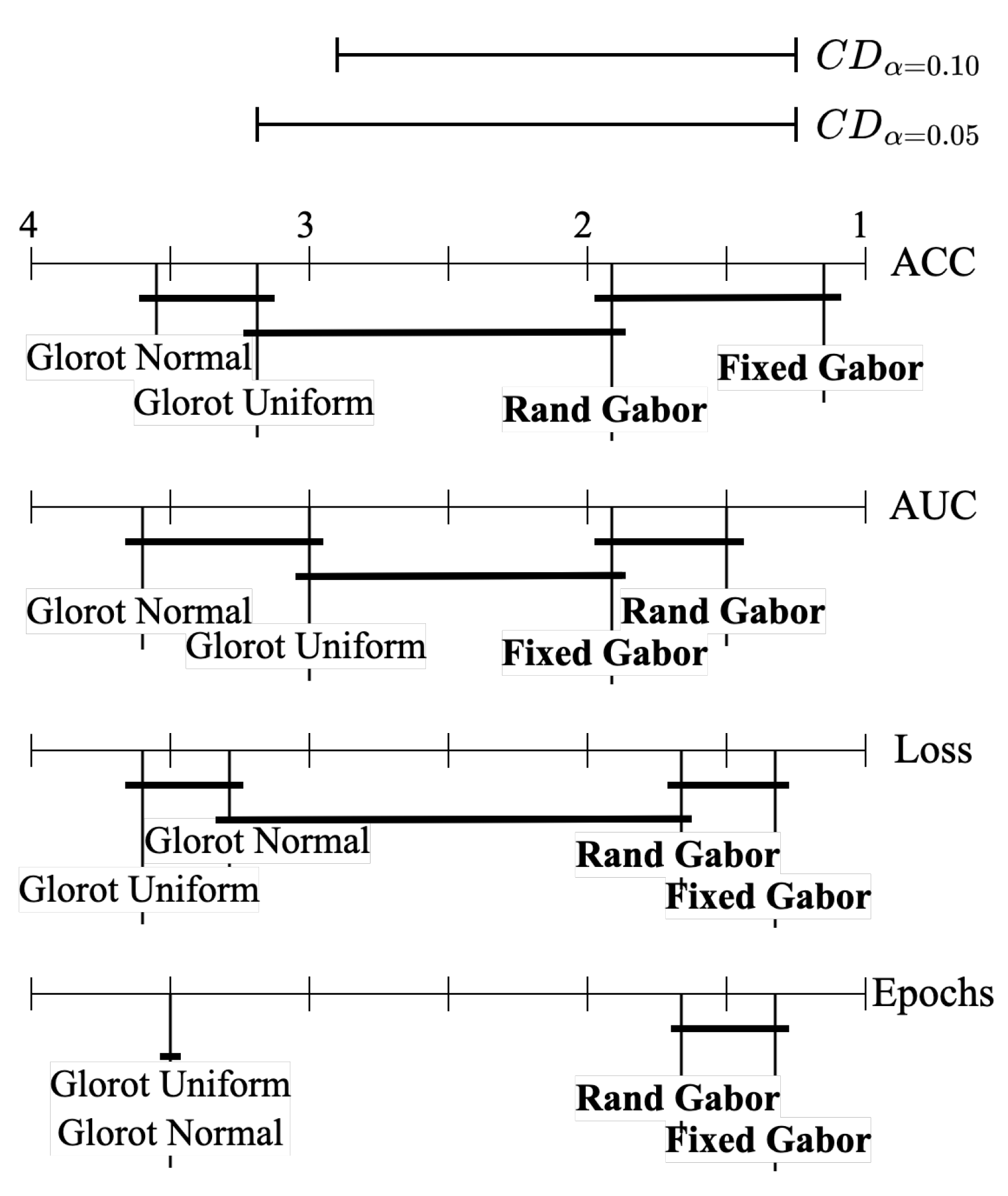
Appendix B. Statistical Analysis

For the statistical analysis that supports Table 4, we performed the following:
χ F 2 = 12 · 6 4 · 5 3.66 2 + 3.33 2 + 1.83 2 + 1.16 2 4 · 5 2 4 , = 15.364 .
F F = 5 · 15.364 6 · 3 15.364 = 29.143 .
The critical value at α = 0.01 is 5.417. We reject H 0 with 99% confidence. The critical differences are:
C D α = 0.05 = 2.569 4 · 5 6 · 6 = 1.915 .
C D α = 0.10 = 2.291 4 · 5 6 · 6 = 1.708 .
Since the difference in rank between the randomized Gabor filter and the baseline Glorot normal filter is 1.83 and is less than the C D α = 0.10 = 1.708 , we conclude that the Gabor filter is better. Similarly, since the difference in rank between the fixed Gabor filter and the baseline Glorot uniform filter is 2.17 and is less than the C D α = 0.05 = 1.915 , we conclude that the Gabor filter is better.
For the statistical analysis that supports Table 4, we performed the following:
χ F 2 = 12 · 6 4 · 5 3.666 2 + 3 2 + 1.5 2 + 1.833 2 4 · 5 2 4 , = 10.978 .
F F = 5 · 10.978 6 · 3 10.978 = 7.817 .
The critical value at α = 0.01 is 5.417. We reject H 0 with 99% confidence.
Since the difference in rank between the fixed Gabor filter and the baseline Glorot normal filter is 1.83 and is less than the C D α = 0.10 = 1.708 , we conclude that the Gabor filter is better. Similarly, since the difference in rank between the random Gabor filter and the baseline Glorot uniform filter is 1.5 and is less than the C D α = 0.05 = 1.915 , we conclude that the Gabor filter is better.
For the statistical analysis that supports Table 5, we performed the following:
χ F 2 = 12 · 6 4 · 5 3.33 2 + 3.66 2 + 1.66 2 + 1.33 2 4 · 5 2 4 , = 14.763 .
F F = 5 · 14.763 6 · 3 14.763 = 22.804 .
The critical value at α = 0.01 is 5.417. We reject H 0 with 99% confidence.
Since the difference in rank between the fixed Gabor filter and the baseline Glorot normal filter is 2 and is less than the C D α = 0.05 = 1.915 , we conclude that the Gabor filter is better. Similarly, since the difference in rank between the random Gabor filter and the baseline Glorot uniform filter is 2 and is less than the C D α = 0.05 = 1.915 , we conclude that the Gabor filter is better.
For the statistical analysis that supports Table 6, we performed the following:
χ F 2 = 12 · 6 4 · 5 3.5 2 + 3.5 2 + 1.666 2 + 1.333 2 4 · 5 2 4 , = 10.536 .
F F = 5 · 10.536 6 · 3 10.536 = 7.058 .
The critical value at α = 0.01 is 5.417. We reject H 0 with 99% confidence.
Since the difference in rank between the random Gabor filter and the baseline Glorot normal filter is 1.84 and is less than the C D α = 0.10 = 1.708 , we conclude that the Gabor filter is better. Similarly, since the difference in rank between the fixed Gabor filter and the baseline Glorot uniform filter is 2.17 and is less than the C D α = 0.05 = 1.915 , we conclude that the Gabor filter is better.

Appendix C. Additional Experiments

Table A1 and Table A2 provide a comprehensive overview of the improvement in terms of the maximum accuracy and the AUC at the maximum accuracy for the Gabor-initialized CNN in comparison to traditional CNNs. This comparison is made under the constraint that the Gabor-initialized CNN is trained only up to the number of epochs where the traditional CNN reaches its maximum accuracy.
Table A3 and Table A4 present a comparison of the minimum loss and number of epochs required to reach its minimum loss for the Gabor-initialized CNN in relation to the traditional CNN, with the constraint that the Gabor-initialized CNN is trained only up to the number of epochs where the traditional CNN reaches its maximum accuracy.
Table A5, Table A6 and Table A7 summarize the improvement in maximum accuracy, AUC at maximum accuracy, and minimum loss of the Gabor-initialized CNN in comparison to traditional CNNs under the constraint that the receptive filters of the Gabor-initialized CNN are frozen, while the filters in other layers are allowed to change.
Finally, the results of experiments conducted with different kernel sizes of the receptive layer of the CNN and image sizes of the datasets can be found in Table A8, Table A9, Table A10, Table A11, Table A12, Table A13, Table A14, Table A15, Table A16, Table A17, Table A18, Table A19, Table A20, Table A21, Table A22, Table A23, Table A24 and Table A25.
Table A1. Improvement in maximum accuracy of epoch-constrained Gabor-initialized CNN with respect to traditional CNN when training period was constrained to maximum accuracy epoch of traditional CNN. Bold numbers indicate top results.
DatasetBase Maximum AccuracyRandom Gabor FilterRepeated Gabor Filter
MeanStdevMeanStdevMeanStdev
Cats vs. Dogs0.88390.004+0.02120.007+0.02530.006
CIFAR-100.80240.004+0.01970.003+0.02120.005
CIFAR-1000.71320.003+0.00540.005+0.00530.005
Caltech 2560.50850.007+0.01310.008+0.01630.010
Stanford Cars0.23260.070+0.12000.065+0.15760.068
Tiny Imagenet0.51750.004+0.01280.003−0.00080.007
Average0.60970.015+0.03200.015+0.03750.017
Table A2. Improvement in AUC at maximum accuracy of epoch-constrained Gabor-initialized CNN with respect to traditional CNN when training period was constrained to maximum accuracy epoch of traditional CNN. Bold numbers indicate top results.
DatasetBase AUCRandom Gabor FilterRepeated Gabor Filter
MeanStdevMeanStdevMeanStdev
Cats vs. Dogs0.95150.003+0.01290.004+0.01640.004
CIFAR-100.97190.001+0.00330.001+0.00260.001
CIFAR-1000.96210.002+0.00130.002+0.00220.002
Caltech 2560.88850.004+0.00860.004+0.00620.005
Stanford Cars0.80770.026+0.05520.022+0.06450.026
Tiny Imagenet0.93700.003+0.00230.004−0.00100.003
Average0.91980.006+0.01340.006+0.01510.007
Table A3. Improvement in minimum loss of Gabor-initialized CNN with respect to traditional CNN when training period was constrained to minimum loss epoch of traditional CNN. Bold numbers indicate top results.
DatasetBase Minimum LossRandom Gabor FilterRepeated Gabor Filter
MeanStdevMeanStdevMeanStdev
Cats vs. Dogs0.29600.012−0.04060.015−0.05530.013
CIFAR-100.65550.013−0.05170.015−0.05670.013
CIFAR-1001.18230.020−0.01500.038−0.01920.029
Caltech 2562.64280.067−0.09080.038−0.01920.029
Stanford Cars4.18570.356−0.65130.231−0.89130.264
Tiny Imagenet2.73900.014−0.05220.024−0.00270.028
Table A4. Improvement in minimum loss epoch of Gabor-initialized CNN with respect to traditional CNN when training period constrained to minimum loss epoch of traditional CNN. Bold numbers indicate top results.
DatasetBase EpochRandom Gabor FilterRepeated Gabor Filter
MeanStdevMeanStdevMeanStdev
Cats vs. Dogs70.613.5−75.4−149.8
CIFAR-1040.15.5−8.68.1−107.4
CIFAR-10070.26.5−6.23.3−8.87.7
Caltech 25642.15.1−3.52.7−5.23.5
Stanford Cars74.014.9−5.14.4−6.43.9
Tiny Imagenet32.24.6−5.25.6−5.96.1
Table A5. Improvement in maximum accuracy of Gabor-initialized CNN (frozen receptive convolutional layer variant) with respect to traditional CNN. Bold numbers indicate top results.
DatasetBase Maximum AccuracyRandom Gabor FilterRepeated Gabor Filter
MeanStdevMeanStdevMeanStdev
Cats vs. Dogs0.88390.004+0.00290.009+0.01830.005
CIFAR-100.80240.004+0.00860.005−0.00750.007
CIFAR-1000.71320.003+0.00220.004−0.05590.007
Caltech 2560.50850.007+0.00790.011+0.00120.012
Stanford Cars0.23260.070+0.09240.096+0.16620.086
Tiny Imagenet0.51750.004+0.00450.009−0.03910.004
Average0.60970.015+0.01970.022+0.01390.020
Table A6. Improvement in AUC of Gabor-initialized CNN (frozen receptive convolutional layer variant) with respect to traditional CNN. Bold numbers indicate top results.
DatasetBase AUCRandom Gabor FilterRepeated Gabor Filter
MeanStdevMeanStdevMeanStdev
Cats vs. Dogs0.95150.003+0.00200.006+0.01330.002
CIFAR-100.97190.001+0.00120.001−0.00170.002
CIFAR-1000.96210.002−0.00030.003−0.00950.002
Caltech 2560.88850.004+0.00520.007+0.00480.006
Stanford Cars0.80770.026+0.04080.035+0.06840.032
Tiny Imagenet0.93700.003+0.00120.004−0.00810.003
Average0.91980.006+0.00830.009+0.01120.008
Table A7. Improvement in minimum loss of Gabor-initialized CNN (frozen receptive convolutional layer variant) with respect to traditional CNN. Bold numbers indicate top results.
DatasetBase Minimum LossRandom Gabor FilterRepeated Gabor Filter
MeanStdevMeanStdevMeanStdev
Cats vs. Dogs0.29600.012−0.01000.018−0.04750.010
CIFAR-100.65550.013−0.03520.019+0.00860.022
CIFAR-1001.18230.020−0.00990.035+0.24370.037
Caltech 2562.64280.067−0.07940.091−0.04660.068
Stanford Cars4.18570.356−0.62170.502−1.08370.487
Tiny Imagenet2.73900.014−0.2400.027+0.16280.019
Table A8. Improvement in maximum accuracy on Cats vs. Dogs dataset with different kernel sizes and image sizes. Bold numbers indicate top results.
Image SizeGabor ConfigurationKernel Size
3 × 35 × 57 × 79 × 911 × 1113 × 1315 × 15
32 × 32Traditional CNN (Base)0.82610.83030.81650.81430.80350.80370.7869
Random Gabor ( Δ )−0.0202−0.0389−0.0114+0.0036+0.0120+0.0044+0.0094
Repeated Gabor ( Δ )−0.0258−0.0174−0.0170−0.0120−0.0174−0.0020+0.0090
64 × 64Traditional CNN (Base)0.80150.84030.83810.82970.84250.83150.8279
Random Gabor ( Δ )−0.0168+0.0038+0.0100+0.0132+0.0022+0.0128+0.0058
Repeated Gabor ( Δ )+0.0126−0.0070+0.0204+0.0162+0.0044+0.0116+0.0180
128 × 128Traditional CNN (Base)0.86720.90260.89480.90220.89920.88040.8952
Random Gabor ( Δ )+0.0062−0.0138−0.0022+0.0114+0.0150+0.0242+0.0150
Repeated Gabor ( Δ )+0.0134+0.0120+0.0228+0.0144+0.0160+0.0341+0.0216
256 × 256Traditional CNN (Base)0.89320.88920.89260.88620.89240.89160.8870
Random Gabor ( Δ )−0.0170−0.0058−0.0078+0.0076+0.0156+0.0214+0.0142
Repeated Gabor ( Δ )−0.0214+0.0120+0.0142+0.0264+0.0136+0.0170+0.0240
Table A9. Improvement in AUC at maximum accuracy on Cats vs. Dogs dataset with different kernel sizes and image sizes. Bold numbers indicate top results.
Image SizeGabor ConfigurationKernel Size
3 × 35 × 57 × 79 × 911 × 1113 × 1315 × 15
32 × 32Traditional CNN (Base)0.90280.90920.89470.89460.87890.88090.8650
Random Gabor ( Δ )−0.0161−0.0391−0.0076−0.0012+0.0137+0.0024+0.0107
Repeated Gabor ( Δ )−0.0208−0.0149−0.0110−0.0081−0.0110+0.0008+0.0095
64 × 64Traditional CNN (Base)0.89000.92320.92130.90770.92140.91270.9097
Random Gabor ( Δ )−0.0179+0.0027+0.0053+0.0103+0.0022+0.0113+0.0081
Repeated Gabor ( Δ )+0.0090−0.0066+0.0127+0.0146+0.0037+0.0116+0.0139
128 × 128Traditional CNN (Base)0.94610.96900.96410.96700.96510.95570.9638
Random Gabor ( Δ )+0.0032−0.0094−0.0028+0.0071+0.0093+0.0148+0.0094
Repeated Gabor ( Δ )+0.0068+0.0044+0.0118+0.0089+0.0097+0.0188+0.0103
256 × 256Traditional CNN (Base)0.95860.95650.96020.95310.95700.95650.9541
Random Gabor ( Δ )−0.0099−0.0016−0.0056+0.0072+0.0086+0.0139+0.0087
Repeated Gabor ( Δ )−0.0129+0.0054+0.0086+0.0178+0.0085+0.0121+0.0141
Table A10. Improvement in minimum loss on Cats vs. Dogs dataset with different kernel sizes and image sizes. Bold numbers indicate top results.
Image SizeGabor ConfigurationKernel Size
3 × 35 × 57 × 79 × 911 × 1113 × 1315 × 15
32 × 32Traditional CNN (Base)0.70391.02081.37930.89910.85740.97651.0263
Random Gabor ( Δ )−0.0630−0.3510−0.7026−0.2184−0.1522−0.1801+0.1596
Repeated Gabor ( Δ )−0.0696−0.3772−0.6521−0.2515−0.1687−0.1927−0.1891
64 × 64Traditional CNN (Base)0.88840.97170.84480.99051.25971.30661.4466
Random Gabor ( Δ )−0.1744−0.2768−0.1251−0.3048−0.5674−0.4398−0.6611
Repeated Gabor ( Δ )−0.2145−0.2895−0.1689−0.3397−0.5842−0.6421−0.6685
128 × 128Traditional CNN (Base)1.04800.88131.10600.76390.88401.03051.3318
Random Gabor ( Δ )−0.3270−0.0753−0.3405−0.0858−0.1525−0.3765−0.5583
Repeated Gabor ( Δ )−0.4209−0.2144−0.4912−0.2167−0.2957−0.3765−0.7697
256 × 256Traditional CNN (Base)1.12610.63740.70550.72331.14260.84590.8025
Random Gabor ( Δ )−0.4575−0.0646−0.0882−0.0916−0.5824−0.2015−0.2225
Repeated Gabor ( Δ )−0.4516−0.0561+0.0252−0.0221−0.5944−0.0720−0.1276
Table A11. Improvement in maximum accuracy on CIFAR-10 dataset with different kernel sizes and image sizes. Bold numbers indicate top results.
Image SizeGabor ConfigurationKernel Size
3 × 35 × 57 × 79 × 911 × 1113 × 1315 × 15
32 × 32Traditional CNN (Base)0.78180.78960.79290.77120.77130.77440.7654
Random Gabor ( Δ )−0.0049−0.0090−0.0122+0.0143+0.0124+0.0089+0.0101
Repeated Gabor ( Δ )−0.0037−0.0028−0.0087+0.0283+0.0164+0.0234+0.0155
64 × 64Traditional CNN (Base)0.70860.72570.71990.72070.71150.72030.7219
Random Gabor ( Δ )−0.0076−0.0129+0.0077+0.0143+0.0279+0.0393+0.0403
Repeated Gabor ( Δ )−0.0098−0.0107+0.0206+0.0348+0.0466+0.0416+0.0394
128 × 128Traditional CNN (Base)0.79360.79880.80070.79300.79890.80040.8067
Random Gabor ( Δ )+0.0086+0.0073+0.0146+0.0258+0.0228+0.0271+0.0177
Repeated Gabor ( Δ )+0.0093+0.0113+0.0134+0.0273+0.0281+0.0199+0.0142
Table A12. Improvement in AUC at maximum accuracy on CIFAR-10 dataset with different kernel sizes and image sizes. Bold numbers indicate top results.
Image SizeGabor ConfigurationKernel Size
3 × 35 × 57 × 79 × 911 × 1113 × 1315 × 15
32 × 32Traditional CNN (Base)0.97590.97730.97770.97440.97340.97370.9722
Random Gabor ( Δ )−0.0011−0.0011−0.0027+0.0018+0.0023+0.0019+0.0018
Repeated Gabor ( Δ )−0.0010−0.0006−0.0019+0.0036+0.0037+0.0034+0.0021
64 × 64Traditional CNN (Base)0.95750.96150.96060.96140.95980.96210.9623
Random Gabor ( Δ )−0.0026−0.0019+0.0020+0.0032+0.0069+0.0073+0.0081
Repeated Gabor ( Δ )−0.0018−0.0006+0.0050+0.0080+0.0104+0.0086+0.0076
128 × 128Traditional CNN (Base)0.97300.97240.97340.97250.97370.97330.9746
Random Gabor ( Δ )+0.0008+0.0017+0.0011+0.0023+0.0023+0.0047+0.0033
Repeated Gabor ( Δ )+0.0005+0.0029+0.0021+0.0044+0.0031+0.0023+0.0015
Table A13. Improvement in minimum loss on CIFAR-10 dataset with different kernel sizes and image sizes. Bold numbers indicate top results.
Image SizeGabor ConfigurationKernel Size
3 × 35 × 57 × 79 × 911 × 1113 × 1315 × 15
32 × 32Traditional CNN (Base)1.47641.56821.96941.91441.66721.59352.1591
Random Gabor ( Δ )−0.1391−0.2193−0.5082−0.5611−0.1535−0.1015−0.6806
Repeated Gabor ( Δ )−0.0672−0.1756−0.6604−0.6354−0.0718−0.1837−0.8144
64 × 64Traditional CNN (Base)1.64601.91602.30011.63421.63781.89212.0575
Random Gabor ( Δ )−0.0266−0.3585−0.6622−0.0978−0.1412−0.2156−0.4911
Repeated Gabor ( Δ )+0.0670−0.3258−0.7804−0.0624−0.1956+0.3132−0.3499
128 × 128Traditional CNN (Base)1.49202.26841.27441.34571.36871.72871.4233
Random Gabor ( Δ )−0.2609−1.1010−0.0477−0.1184−0.1824−0.3236−0.0045
Repeated Gabor ( Δ )−0.2781−1.0944+0.2863−0.1774−0.2432−0.1496−0.0947
Table A14. Improvement in maximum accuracy on CIFAR-100 dataset with different kernel sizes and image sizes. Bold numbers indicate top results.
Image SizeGabor ConfigurationKernel Size
3 × 35 × 57 × 79 × 911 × 1113 × 1315 × 15
32 × 32Traditional CNN (Base)0.58420.57400.58540.54880.56050.56780.5590
Random Gabor ( Δ )−0.0237+0.0114−0.0281+0.0192+0.0201−0.0139+0.0081
Repeated Gabor ( Δ )−0.0189+0.0003−0.0021+0.0023+0.0004−0.0086−0.0029
64 × 64Traditional CNN (Base)0.68030.68690.68070.68660.68980.68860.6867
Random Gabor ( Δ )+0.0007+0.0025−0.0007−0.0015−0.0087−0.0094−0.0015
Repeated Gabor ( Δ )+0.0039+0.0018+0.0027−0.0028−0.0080−0.0010−0.0006
128 × 128Traditional CNN (Base)0.71440.70650.71620.71640.71380.71230.7112
Random Gabor ( Δ )−0.0060+0.0037+0.0018+0.0002+0.0012+0.00730.0059
Repeated Gabor ( Δ )+0.0017+0.0106−0.0070−0.0041+0.0040+0.0086+0.0145
Table A15. Improvement in AUC at maximum accuracy on CIFAR-100 dataset with different kernel sizes and image sizes. Bold numbers indicate top results.
Image SizeGabor ConfigurationKernel Size
3 × 35 × 57 × 79 × 911 × 1113 × 1315 × 15
32 × 32Traditional CNN (Base)0.95500.95030.95300.95250.95110.95140.9512
Random Gabor ( Δ )−0.0025+0.0035+0.0003−0.0028+0.0023−0.0007−0.0004
Repeated Gabor ( Δ )−0.0036+0.0018−0.0006+0.0025−0.0019+0.0020−0.0006
64 × 64Traditional CNN (Base)0.96360.96520.96590.96280.96550.96430.9652
Random Gabor ( Δ )+0.0008+0.0002−0.0009+0.0030−0.0006+0.0025+0.0007
Repeated Gabor ( Δ )−0.0004−0.0004−0.0007+0.0027−0.0012+0.0021+0.0006
128 × 128Traditional CNN (Base)0.96940.96860.96840.96900.96820.96910.9682
Random Gabor ( Δ )+0.0008+0.0002+0.0010+0.0021+0.0028+0.0000+0.0016
Repeated Gabor ( Δ )+0.0002+0.0011+0.0030+0.0013+0.0010+0.0007+0.0029
Table A16. Improvement in minimum loss on CIFAR-100 dataset with different kernel sizes and image sizes. Bold numbers indicate top results.
Image SizeGabor ConfigurationKernel Size
3 × 35 × 57 × 79 × 911 × 1113 × 1315 × 15
32 × 32Traditional CNN (Base)4.33994.56084.08805.94394.14164.25995.1038
Random Gabor ( Δ )+0.1598−0.6657−0.0989−1.7213+0.1809−0.2785+2.1429
Repeated Gabor ( Δ )+0.4380−0.4634+0.7734−1.5532+0.5421+0.2966−1.1574
64 × 64Traditional CNN (Base)3.63483.74673.57153.80463.81584.05754.0832
Random Gabor ( Δ )+0.1774−0.0744+0.0242−0.3521+0.2289+0.1263+0.2179
Repeated Gabor ( Δ )+0.5789+0.3015+1.7995−0.0274+0.1685+0.8609+0.1275
128 × 128Traditional CNN (Base)3.49364.13854.16665.11513.76943.58854.0887
Random Gabor ( Δ )+0.2320−0.2233−0.6036−1.3428+0.9635+0.0513−0.0090
Repeated Gabor ( Δ )+0.4857−0.2240−0.1239−0.6645+0.0184−0.0016+0.1811
Table A17. Improvement in maximum accuracy on Caltech 256 dataset with different kernel sizes and image sizes. Bold numbers indicate top results.
Image SizeGabor ConfigurationKernel Size
3 × 35 × 57 × 79 × 911 × 1113 × 1315 × 15
32 × 32Traditional CNN (Base)0.30860.30840.30220.30960.30610.30990.2978
Random Gabor ( Δ )−0.0007+0.0002+0.0195+0.0106+0.0064+0.0010+0.0008
Repeated Gabor ( Δ )+0.0123+0.0020+0.0146+0.0115+0.0056+0.0008−0.0005
64 × 64Traditional CNN (Base)0.42960.43880.43750.44040.44030.43800.4313
Random Gabor ( Δ )−0.0090−0.0028+0.0113+0.0025−0.0116+0.0119+0.0214
Repeated Gabor ( Δ )+0.0039−0.0054+0.0082+0.0072+0.0113+0.0059+0.0059
128 × 128Traditional CNN (Base)0.50280.50250.53500.52000.51130.51950.5092
Random Gabor ( Δ )+0.0151+0.0208+0.0008+0.0026+0.0211+0.0061+0.0041
Repeated Gabor ( Δ )+0.0195+0.0128−0.0043+0.0036+0.0188+0.0051+0.0198
Table A18. Improvement in AUC at maximum accuracy on Caltech 256 dataset with different kernel sizes and image sizes. Bold numbers indicate top results.
Image SizeGabor ConfigurationKernel Size
3 × 35 × 57 × 79 × 911 × 1113 × 1315 × 15
32 × 32Traditional CNN (Base)0.84810.84190.85130.85740.84540.84740.8392
Random Gabor ( Δ )−0.0021+0.0162+0.0019−0.0027+0.0050+0.0003+0.0057
Repeated Gabor ( Δ )+0.0055+0.0095−0.0030+0.0005+0.0131+0.0037+0.0069
64 × 64Traditional CNN (Base)0.87410.88530.88460.88530.88370.88480.8840
Random Gabor ( Δ )+0.0026−0.0037+0.0036+0.0033−0.0010+0.0060−0.0001
Repeated Gabor ( Δ )+0.0037−0.0028−0.0007+0.0050+0.0114+0.0034+0.0041
128 × 128Traditional CNN (Base)0.90340.90970.90620.90360.90460.90490.9021
Random Gabor ( Δ )+0.0053−0.0004+0.0072+0.0020+0.0006−0.0059+0.0036
Repeated Gabor ( Δ )+0.0050+0.0002+0.0010+0.0028+0.0045+0.0044+0.0054
Table A19. Improvement in minimum loss on Caltech 256 dataset with different kernel sizes and image sizes. Bold numbers indicate top results.
Image SizeGabor ConfigurationKernel Size
3 × 35 × 57 × 79 × 911 × 1113 × 1315 × 15
32 × 32Traditional CNN (Base)8.18926.25507.04107.87058.504611.15195.8391
Random Gabor ( Δ )−2.5809+0.6026−1.6581−2.3008+0.8493−0.4026−0.3982
Repeated Gabor ( Δ )−1.6821+1.8756−1.0074−1.6438−0.5016−5.2436+2.1425
64 × 64Traditional CNN (Base)6.37748.14256.87216.73147.03048.63865.2090
Random Gabor ( Δ )−0.8742−3.0356−1.2754−1.3800−1.0103−2.7627+0.8800
Repeated Gabor ( Δ )−1.1548−2.6945+3.0506−0.1708+5.0498−2.1193+0.7651
128 × 128Traditional CNN (Base)4.90905.197813.06246.81606.34267.12367.1915
Random Gabor ( Δ )+0.3547+0.1951−8.0269−1.6014−1.3128−1.7678−1.8235
Repeated Gabor ( Δ )+0.7467+0.3598−7.7013−0.7981−0.6349+1.1454−1.4903
Table A20. Improvement in maximum accuracy on Stanford Cars dataset with different kernel sizes and image sizes. Bold numbers indicate top results.
Image SizeGabor ConfigurationKernel Size
3 × 35 × 57 × 79 × 911 × 1113 × 1315 × 15
32 × 32Traditional CNN (Base)0.04930.04260.04420.04250.03040.03340.0300
Random Gabor ( Δ )−0.0088+0.0090−0.0002+0.0060+0.0133+0.0076+0.0009
Repeated Gabor ( Δ )+0.0051+0.0024+0.0004+0.0059+0.0152+0.0115+0.0139
64 × 64Traditional CNN (Base)0.17740.16020.14980.13500.13860.08180.1143
Random Gabor ( Δ )−0.0330+0.0081+0.0015+0.0019−0.0162+0.0436−0.0009
Repeated Gabor ( Δ )−0.0339+0.0117+0.0326+0.0281−0.0092+0.0524+0.0410
128 × 128Traditional CNN (Base)0.41030.38790.41800.35980.30100.31020.3517
Random Gabor ( Δ )−0.0151+0.0396+0.0157+0.0802+0.1398+0.1930+0.0600
Repeated Gabor ( Δ )−0.0818+0.0274+0.0005+0.0029+0.1313+0.0788+0.0648
Table A21. Improvement in AUC at maximum accuracy on Stanford Cars dataset with different kernel sizes and image sizes. Bold numbers indicate top results.
Image SizeGabor ConfigurationKernel Size
3 × 35 × 57 × 79 × 911 × 1113 × 1315 × 15
32 × 32Traditional CNN (Base)0.71070.69700.71140.69070.62900.64270.6325
Random Gabor ( Δ )−0.0198+0.0019−0.0198+0.0009+0.0526+0.0292+0.0041
Repeated Gabor ( Δ )+0.0111−0.0038−0.0106+0.0173+0.0705+0.0448+0.0568
64 × 64Traditional CNN (Base)0.82110.80460.79110.78150.77130.72550.7472
Random Gabor ( Δ )−0.0173−0.0063+0.0018+0.0030−0.0056+0.0358+0.0146
Repeated Gabor ( Δ )−0.0150−0.0046+0.0154+0.0165+0.0045+0.0528+0.0388
128 × 128Traditional CNN (Base)0.87360.88310.87230.88080.83690.83440.8811
Random Gabor ( Δ )+0.0020+0.0020+0.0180+0.0033+0.0455+0.0458+0.0032
Repeated Gabor ( Δ )+0.0063+0.0017+0.0028+0.0030+0.0515+0.0278+0.0035
Table A22. Improvement in minimum loss on Stanford Cars dataset with different kernel sizes and image sizes. Bold numbers indicate top results.
Image SizeGabor ConfigurationKernel Size
3 × 35 × 57 × 79 × 911 × 1113 × 1315 × 15
32 × 32Traditional CNN (Base)7.320347.55998.87509.270222.82317.16489.1182
Random Gabor ( Δ )+12.3424−37.8715+3.6937+3.4808−15.7108+0.3171+0.4810
Repeated Gabor ( Δ )+7.1468−37.3148−2.6179+6.2107−4.7338+5.3186+7.1548
64 × 64Traditional CNN (Base)24.18747.346014.208110.478016.097417.061420.6991
Random Gabor ( Δ )−13.0682+1.0896−6.3144+1.3075−3.0181−4.1803−0.5565
Repeated Gabor ( Δ )−16.0293+13.3526+13.5375+2.7611−1.1857−0.2307−3.6890
128 × 128Traditional CNN (Base)18.813636.223018.17276.69716.591573.80666.7081
Random Gabor ( Δ )−1.3699−26.1808−9.9487+9.0980+4.3474−66.8044+7.0920
Repeated Gabor ( Δ )−4.3315−23.0504−9.2398+4.6752+34.7256−62.0934+4.2712
Table A23. Improvement in maximum accuracy on Tiny Imagenet dataset with different kernel sizes and image sizes. Bold numbers indicate top results.
Image SizeGabor ConfigurationKernel Size
3 × 35 × 57 × 79 × 911 × 1113 × 1315 × 15
32 × 32Traditional CNN (Base)0.39210.39500.38320.37120.36710.36490.3543
Random Gabor ( Δ )−0.0077−0.0029−0.0419−0.0223−0.0294−0.0340−0.0083
Repeated Gabor ( Δ )−0.0050−0.0465−0.0462−0.0453−0.0401−0.0612−0.0410
64 × 64Traditional CNN (Base)0.48060.48240.47390.46990.46590.46620.4562
Random Gabor ( Δ )+0.0102−0.0021−0.0041−0.0072−0.0102+0.0002+0.0152
Repeated Gabor ( Δ )−0.0037−0.0390−0.0186+0.0004−0.0244−0.0229−0.0021
128 × 128Traditional CNN (Base)0.51990.52330.52410.52160.52290.52180.5104
Random Gabor ( Δ )+0.0113+0.0056+0.0081−0.0031−0.0018+0.0056+0.0170
Repeated Gabor ( Δ )−0.0066−0.0153−0.0411−0.0126−0.0142−0.0099+0.0060
Table A24. Improvement in AUC at maximum accuracy on Tiny Imagenet dataset with different kernel sizes and image sizes. Bold numbers indicate top results.
Image SizeGabor ConfigurationKernel Size
3 × 35 × 57 × 79 × 911 × 1113 × 1315 × 15
32 × 32Traditional CNN (Base)0.91090.91130.90620.90560.90110.89910.8979
Random Gabor ( Δ )−0.0002−0.0054−0.0118−0.0109−0.0079−0.0098−0.0006
Repeated Gabor ( Δ )−0.0038−0.0181−0.0082−0.0163−0.0103−0.0172−0.0175
64 × 64Traditional CNN (Base)0.93610.93190.93330.93120.93080.92940.9262
Random Gabor ( Δ )−0.0031+0.0008−0.0026+0.0002−0.0033−0.0006+0.0037
Repeated Gabor ( Δ )−0.0093−0.0050−0.0094−0.0021−0.0039−0.0078−0.0018
128 × 128Traditional CNN (Base)0.94350.94180.94380.94320.94390.94280.9427
Random Gabor ( Δ )−0.0006+0.0011−0.0013−0.0017−0.0014−0.0009+0.0013
Repeated Gabor ( Δ )−0.0065−0.0068−0.0091−0.0089−0.0061−0.0056−0.0023
Table A25. Improvement in minimum loss on Tiny Imagenet dataset with different kernel sizes and image sizes. Bold numbers indicate top results.
Image SizeGabor ConfigurationKernel Size
3 × 35 × 57 × 79 × 911 × 1113 × 1315 × 15
32 × 32Traditional CNN (Base)5.29125.22735.23225.14885.16895.20505.1729
Random Gabor ( Δ )−0.2901−0.2618−0.2595−0.2248−0.1753−0.1808−0.1660
Repeated Gabor ( Δ )−0.0636−0.0202−0.0505−0.0025−0.0429−0.0107−0.0384
64 × 64Traditional CNN (Base)5.10145.14285.11985.12465.08475.12345.0616
Random Gabor ( Δ )−0.2692−0.2719−0.2538−0.2102−0.2546−0.1730−0.1027
Repeated Gabor ( Δ )+0.1317+0.0625−0.0146−0.0464+0.0509−0.0955−0.0103
128 × 128Traditional CNN (Base)5.06595.06165.05845.02575.00925.06735.2985
Random Gabor ( Δ )−0.2046−0.2492−0.3288−0.1116+0.0950−0.0409−0.5205
Repeated Gabor ( Δ )+0.1017+0.0927+0.0865+0.0545+0.0739−0.0492−0.3941

References

  1. Munawar, H.S.; Aggarwal, R.; Qadir, Z.; Khan, S.I.; Kouzani, A.Z.; Mahmud, M.P. A gabor filter-based protocol for automated image-based building detection. Buildings 2021, 11, 302. [Google Scholar] [CrossRef]
  2. Tadic, V.; Kiraly, Z.; Odry, P.; Trpovski, Z.; Loncar-Turukalo, T. Comparison of Gabor filter bank and fuzzified Gabor filter for license plate detection. Acta Polytech. Hung. 2020, 17, 61–81. [Google Scholar] [CrossRef]
  3. Lahmyed, R.; Ansari, M.E.; Kerkaou, Z. Automatic road sign detection and recognition based on neural network. Soft Comput. 2022, 26, 1743–1764. [Google Scholar] [CrossRef]
  4. Kadhim, R.R.; Kamil, M.Y. Breast invasive ductal carcinoma diagnosis using machine learning models and Gabor filter method of histology images. Int. J. Reconfig. Embed. Syst. 2023, 12, 9. [Google Scholar] [CrossRef]
  5. Ibtissam, Z.; Brahim, C.; Lhoussaine, M. Building detection using local Gabor feature. Int. J. Comput. Appl. 2018, 181, 17–20. [Google Scholar] [CrossRef]
  6. Kristanto, S.P.; Hakim, L.; Yusuf, D. Kmeans Clustering Segmentation on Water Microbial Image with Color and Texture Feature Extraction. Build. Inform. Technol. Sci. (BITS) 2022, 4, 1317–1324. [Google Scholar] [CrossRef]
  7. Liu, C.; Li, J.; He, L.; Plaza, A.; Li, S.; Li, B. Naive Gabor networks for hyperspectral image classification. IEEE Trans. Neural Netw. Learn. Syst. 2020, 32, 376–390. [Google Scholar] [CrossRef]
  8. Chen, C.; Li, W.; Su, H.; Liu, K. Spectral-spatial classification of hyperspectral image based on kernel extreme learning machine. Remote Sens. 2014, 6, 5795–5814. [Google Scholar] [CrossRef]
  9. Dunn, D.; Higgins, W.E.; Wakeley, J. Texture segmentation using 2-D Gabor elementary functions. IEEE Trans. Pattern Anal. Mach. Intell. 1994, 16, 130–149. [Google Scholar] [CrossRef]
  10. Dunn, D.; Higgins, W.E. Optimal Gabor filters for texture segmentation. IEEE Trans. Image Process. 1995, 4, 947–964. [Google Scholar] [CrossRef]
  11. Jain, A.K.; Ratha, N.K.; Lakshmanan, S. Object detection using gabor filters. Pattern Recognit. 1997, 30, 295–309. [Google Scholar] [CrossRef]
  12. Hosseini, S.; Lee, S.H.; Kwon, H.J.; Koo, H.I.; Cho, N.I. Age and gender classification using wide convolutional neural network and Gabor filter. In Proceedings of the 2018 International Workshop on Advanced Image Technology (IWAIT), Chiang Mai, Thailand, 7–9 January 2018; pp. 1–3. [Google Scholar]
  13. Nunes, C.F.G.; Pádua, F.L.C. A Local Feature Descriptor Based on Log-Gabor Filters for Keypoint Matching in Multispectral Images. IEEE Geosci. Remote Sens. Lett. 2017, 14, 1850–1854. [Google Scholar] [CrossRef]
  14. Premana, A.; Wijaya, A.P.; Soeleman, M.A. Image segmentation using Gabor filter and K-means clustering method. In Proceedings of the 2017 International Seminar on Application for Technology of Information and Communication (iSemantic), Semarang, Indonesia, 7–8 October 2017; pp. 95–99. [Google Scholar]
  15. Li, Z.; Ma, H.; Liu, Z. Road Lane Detection with Gabor Filters. In Proceedings of the 2016 International Conference on Information System and Artificial Intelligence (ISAI), Hong Kong, China, 24–26 June 2016; pp. 436–440. [Google Scholar]
  16. Dosovitskiy, A.; Beyer, L.; Kolesnikov, A.; Weissenborn, D.; Zhai, X.; Unterthiner, T.; Dehghani, M.; Minderer, M.; Heigold, G.; Gelly, S.; et al. An image is worth 16x16 words: Transformers for image recognition at scale. arXiv 2020, arXiv:2010.11929. [Google Scholar]
  17. Trockman, A.; Kolter, J.Z. Patches are all you need? arXiv 2022, arXiv:2201.09792. [Google Scholar]
  18. Lawrence, S.; Giles, C.L.; Tsoi, A.C.; Back, A.D. Face recognition: A convolutional neural-network approach. IEEE Trans. Neural Netw. 1997, 8, 98–113. [Google Scholar] [CrossRef]
  19. Krizhevsky, A.; Sutskever, I.; Hinton, G.E. ImageNet Classification with Deep Convolutional Neural Networks. In Advances in Neural Information Processing Systems 25; Pereira, F., Burges, C.J.C., Bottou, L., Weinberger, K.Q., Eds.; Curran Associates, Inc.: Red Hook, NY, USA, 2012; pp. 1097–1105. [Google Scholar]
  20. Anwar, S.; Hwang, K.; Sung, W. Fixed point optimization of deep convolutional neural networks for object recognition. In Proceedings of the 2015 IEEE International Conference on Acoustics, Speech and Signal Processing (ICASSP), South Brisbane, QLD, Australia, 19–24 April 2015; pp. 1131–1135. [Google Scholar]
  21. Ciresan, D.C.; Meier, U.; Masci, J.; Gambardella, L.M.; Schmidhuber, J. Flexible, High Performance Convolutional Neural Networks for Image Classification. In Proceedings of the Twenty-Second International Joint Conference on Artificial Intelligence, Barcelona, Catalonia, Spain, 16–22 July 2011. [Google Scholar]
  22. Kawano, Y.; Yanai, K. Food Image Recognition with Deep Convolutional Features. In Proceedings of the 2014 ACM International Joint Conference on Pervasive and Ubiquitous Computing: Adjunct Publication (UbiComp’14 Adjunct), Seattle, WA, USA, 13–17 September 2014; pp. 589–593. [Google Scholar] [CrossRef]
  23. Szarvas, M.; Yoshizawa, A.; Yamamoto, M.; Ogata, J. Pedestrian detection with convolutional neural networks. In Proceedings of the IEEE Proceedings. Intelligent Vehicles Symposium, Las Vegas, NV, USA, 6–8 June 2005; pp. 224–229. [Google Scholar]
  24. Maturana, D.; Scherer, S. VoxNet: A 3D Convolutional Neural Network for real-time object recognition. In Proceedings of the 2015 IEEE/RSJ International Conference on Intelligent Robots and Systems (IROS), Hamburg, Germany, 28 September–2 October 2015; pp. 922–928. [Google Scholar]
  25. Zhi, S.; Liu, Y.; Li, X.; Guo, Y. LightNet: A Lightweight 3D Convolutional Neural Network for Real-Time 3D Object Recognition. In Proceedings of the Workshop on 3D Object Retrieval (3Dor ’17), Goslar, Germany, 23–24 April 2017; pp. 9–16. [Google Scholar] [CrossRef]
  26. Luan, S.; Chen, C.; Zhang, B.; Han, J.; Liu, J. Gabor Convolutional Networks. IEEE Trans. Image Process. 2018, 27, 4357–4366. [Google Scholar] [CrossRef]
  27. Liu, C.; Ding, W.; Wang, X.; Zhang, B. Hybrid Gabor Convolutional Networks. Pattern Recognit. Lett. 2018, 116, 164–169. [Google Scholar] [CrossRef]
  28. Molaei, S.; Shiri, M.; Horan, K.; Kahrobaei, D.; Nallamothu, B.; Najarian, K. Deep Convolutional Neural Networks for left ventricle segmentation. In Proceedings of the 2017 39th Annual International Conference of the IEEE Engineering in Medicine and Biology Society (EMBC), Jeju, Republic of Korea, 11–15 July 2017; pp. 668–671. [Google Scholar]
  29. Rai, M.; Rivas, P. A review of convolutional neural networks and gabor filters in object recognition. In Proceedings of the 2020 International Conference on Computational Science and Computational Intelligence (CSCI), Las Vegas, NV, USA, 16–18 December 2020; pp. 1560–1567. [Google Scholar]
  30. He, K.; Zhang, X.; Ren, S.; Sun, J. Deep residual learning for image recognition. In Proceedings of the IEEE Conference on Computer Vision and Pattern Recognition, Las Vegas, NV, USA, 26 June–1 July 2016; pp. 770–778. [Google Scholar]
  31. He, K.; Zhang, X.; Ren, S.; Sun, J. Identity mappings in deep residual networks. In Computer Vision–ECCV 2016: Proceedings of the 14th European Conference, Amsterdam, The Netherlands, 11–14 October 2016; Proceedings, Part IV 14; Springer: Cham, Switzerland, 2016; pp. 630–645. [Google Scholar]
  32. Huang, G.; Liu, Z.; Van Der Maaten, L.; Weinberger, K.Q. Densely connected convolutional networks. In Proceedings of the IEEE Conference on Computer Vision and Pattern Recognition, Honolulu, HI, USA, 21–26 July 2017; pp. 4700–4708. [Google Scholar]
  33. Gabor, D. Theory of communication. J. Inst. Elec. Eng. 1946, 93, 429–457. [Google Scholar] [CrossRef]
  34. Daugman, J. Uncertainty relation for resolution in space, spatial frequency and orientation optimized by two-dimensional visual cortical filters. J. Opt. Soc. Am. A. 1985, 2, 1160–1169. [Google Scholar] [CrossRef]
  35. Kumar, A.; Pang, G.K.H. Defect detection in textured materials using Gabor filters. IEEE Trans. Ind. Appl. 2002, 38, 425–440. [Google Scholar] [CrossRef]
  36. Jing, J.; Fang, X.; Li, P. Automated Fabric Defect Detection Based on Multiple Gabor Filters and KPCA. Int. J. Multimed. Ubiquitous Eng. 2016, 11, 93–106. [Google Scholar] [CrossRef]
  37. El-Sayed, M.A.; Hassaballah, M.; Abdel-Latif, M.A. Identity Verification of Individuals Based on Retinal Features Using Gabor Filters and SVM. J. Signal Inf. Process. 2016, 7, 49. [Google Scholar] [CrossRef]
  38. Gornale, S.; Patil, A.; Veersheety, C. Fingerprint based Gender Identification using Discrete Wavelet Transform and Gabor Filters. Int. J. Comput. Appl. 2016, 152, 8887. [Google Scholar] [CrossRef]
  39. Rizvi, S.T.H.; Cabodi, G.; Gusmao, P.; Francini, G. Gabor filter based image representation for object classification. In Proceedings of the 2016 International Conference on Control, Decision and Information Technologies (CoDIT), Saint Julian’s, Malta, 6–8 April 2016; pp. 628–632. [Google Scholar]
  40. Avinash, S.; Manjunath, K.; Kumar, S.S. An improved image processing analysis for the detection of lung cancer using Gabor filters and watershed segmentation technique. In Proceedings of the 2016 International Conference on Inventive Computation Technologies (ICICT), Coimbatore, India, 26–27 August 2016; Volume 3, pp. 1–6. [Google Scholar]
  41. Daamouche, A.; Fares, D.; Maalem, I.; Zemmouri, K. Unsupervised Method for Building Detection using Gabor Filters. In Proceedings of the Special Issue of the 2nd International Conference on Computational and Experimental Science and Engineering (ICCESEN 2015), Kemer, Antalya, Turkey, 14–19 October 2016; Volume 130. [Google Scholar]
  42. Hemalatha, G.; Sumathi, C.P. Preprocessing techniques of facial image with Median and Gabor filters. In Proceedings of the 2016 International Conference on Information Communication and Embedded Systems (ICICES), Chennai, India, 25–26 February 2016; pp. 1–6. [Google Scholar]
  43. Lefkovits, S.; Lefkovits, L.; Emerich, S. Detecting the eye and its openness with Gabor filters. In Proceedings of the 2017 5th International Symposium on Digital Forensic and Security (ISDFS), Tirgu Mures, Romania, 26–28 April 2017; pp. 1–5. [Google Scholar]
  44. Viola, P.; Jones, M. Rapid object detection using a boosted cascade of simple features. In Proceedings of the 2001 IEEE Computer Society Conference on Computer Vision and Pattern Recognition (CVPR 2001), Kauai, HI, USA, 8–14 December 2001; Volume 1, p. I. [Google Scholar]
  45. Pumlumchiak, T.; Vittayakorn, S. Facial expression recognition using local Gabor filters and PCA plus LDA. In Proceedings of the 2017 9th International Conference on Information Technology and Electrical Engineering (ICITEE), Phuket, Thailand, 12–13 October 2017; pp. 1–6. [Google Scholar]
  46. Mahmood, M.; Jalal, A.; Evans, H.A. Facial Expression Recognition in Image Sequences Using 1D Transform and Gabor Wavelet Transform. In Proceedings of the 2018 International Conference on Applied and Engineering Mathematics (ICAEM), Taxila, Pakistan, 4–5 September 2018; pp. 1–6. [Google Scholar]
  47. Low, C.; Teoh, A.B.; Ng, C. Multi-fold Gabor filter convolution descriptor for face recognition. In Proceedings of the 2016 IEEE International Conference on Acoustics, Speech and Signal Processing (ICASSP), Shanghai, China, 20–25 March 2016; pp. 2094–2098. [Google Scholar]
  48. Lei, Z.; Pietikäinen, M.; Li, S.Z. Learning Discriminant Face Descriptor. IEEE Trans. Pattern Anal. Mach. Intell. 2014, 36, 289–302. [Google Scholar] [PubMed]
  49. Lu, J.; Liong, V.E.; Zhou, X.; Zhou, J. Learning Compact Binary Face Descriptor for Face Recognition. IEEE Trans. Pattern Anal. Mach. Intell. 2015, 37, 2041–2056. [Google Scholar] [CrossRef] [PubMed]
  50. Nava, R.; Escalante-Ramirez, B.; Cristobal, G. Texture Image Retrieval Based on Log-Gabor Features. In Progress in Pattern Recognition, Image Analysis, Computer Vision, and Appplications; Springer: Berlin/Heidelberg, Germany, 2012; Volume 7441, pp. 414–421. [Google Scholar]
  51. Liu, X.; Lao, J.B.; Pang, J.S. Feature Point Matching Based on Distinct Wavelength Phase Congruency and Log-Gabor Filters in Infrared and Visible Images. Sensors 2019, 19, 4244. [Google Scholar] [CrossRef]
  52. Fan, Z.; Zhang, S.; Mei, J.; Liu, M. Recognition of Woven Fabric based on Image Processing and Gabor Filters. In Proceedings of the 2017 IEEE 7th Annual International Conference on CYBER Technology in Automation, Control, and Intelligent Systems (CYBER), Honolulu, HI, USA, 31 July–4 August 2017; pp. 996–1000. [Google Scholar]
  53. Srivastava, G.; Srivastava, R. Salient object detection using background subtraction, Gabor filters, objectness and minimum directional backgroundness. J. Vis. Commun. Image Represent. 2019, 62, 330–339. [Google Scholar] [CrossRef]
  54. Khaleefah, S.H.; Mostafa, S.A.; Mustapha, A.; Nasrudin, M.F. The ideal effect of Gabor filters and Uniform Local Binary Pattern combinations on deformed scanned paper images. J. King Saud Univ. Comput. Inf. Sci. 2019, 33, 1219–1230. [Google Scholar] [CrossRef]
  55. Le Cun, Y.; Boser, B.; Denker, J.S.; Henderson, D.; Howard, R.E.; Hubbard, W.; Jackel, L.D. Handwritten Digit Recognition with a Back-Propagation Network. In Proceedings of the Advances in Neural Information Processing Systems, Denver, CO, USA, 26–29 November 1990; pp. 396–404. [Google Scholar]
  56. Schwarz, M.; Schulz, H.; Behnke, S. RGB-D object recognition and pose estimation based on pre-trained convolutional neural network features. In Proceedings of the 2015 IEEE International Conference on Robotics and Automation (ICRA), Seattle, WA, USA, 26–30 May 2015; pp. 1329–1335. [Google Scholar]
  57. Fang, W.; Ding, L.; Zhong, B.; Love, P.E.; Luo, H. Automated detection of workers and heavy equipment on construction sites: A convolutional neural network approach. Adv. Eng. Inform. 2018, 37, 139–149. [Google Scholar] [CrossRef]
  58. Yao, H.; Chuyi, L.; Dan, H.; Weiyu, Y. Gabor Feature Based Convolutional Neural Network for Object Recognition in Natural Scene. In Proceedings of the 2016 3rd International Conference on Information Science and Control Engineering (ICISCE), Beijing, China, 8–10 July 2016; pp. 386–390. [Google Scholar]
  59. Taghi Zadeh, M.M.; Imani, M.; Majidi, B. Fast Facial emotion recognition Using Convolutional Neural Networks and Gabor Filters. In Proceedings of the 2019 5th Conference on Knowledge Based Engineering and Innovation (KBEI), Tehran, Iran, 28 February–1 March 2019; pp. 577–581. [Google Scholar]
  60. Alekseev, A.; Bobe, A. GaborNet: Gabor filters with learnable parameters in deep convolutional neural network. In Proceedings of the 2019 International Conference on Engineering and Telecommunication (EnT), Dolgoprudny, Russia, 20–21 November 2019; pp. 1–4. [Google Scholar]
  61. Demšar, J. Statistical comparisons of classifiers over multiple data sets. J. Mach. Learn. Res. 2006, 7, 1–30. [Google Scholar]
  62. Meshgini, S.; Aghagolzadeh, A.; Seyedarabi, H. Face Recognition Using Gabor Filter Bank, Kernel Principle Component Analysis and Support Vector Machine. Int. J. Comput. Theory Eng. 2012, 4, 767–771. [Google Scholar] [CrossRef]
  63. Glorot, X.; Bengio, Y. Understanding the difficulty of training deep feedforward neural networks. In Proceedings of the Thirteenth International Conference on Artificial Intelligence and Statistics, JMLR Workshop and Conference Proceedings. Chia Laguna Resort, Sardinia, Italy, 13–15 May 2010; pp. 249–256. [Google Scholar]
  64. Rivas, P. Deep Learning for Beginners: A Beginner’s Guide to Getting Up and Running with Deep Learning from Scratch Using Python; Packt Publishing Ltd.: Birmingham, UK, 2020. [Google Scholar]
  65. Elson, J.; Douceur, J.J.; Howell, J.; Saul, J. Asirra: A CAPTCHA that Exploits Interest-Aligned Manual Image Categorization. In Proceedings of the 14th ACM Conference on Computer and Communications Security (CCS), Alexandria, VA, USA, 31 October–2 November 2007; Association for Computing Machinery, Inc.: New York, NY, USA, October 2007. [Google Scholar]
  66. Krizhevsky, A. Learning Multiple Layers of Features from Tiny Images; Technical Report; University of Toronto: Toronto, ON, Canada, 2009. [Google Scholar]
  67. Griffin, G.; Holub, A.; Perona, P. Caltech-256 Object Category Dataset; CalTech Report; California Institute of Technology: Pasadena, CA, USA, 2007. [Google Scholar]
  68. Krause, J.; Stark, M.; Deng, J.; Fei-Fei, L. 3D Object Representations for Fine-Grained Categorization. In Proceedings of the 4th International IEEE Workshop on 3D Representation and Recognition (3dRR-13), Sydney, NSW, Australia, 2–8 December 2013. [Google Scholar]
  69. Russakovsky, O.; Deng, J.; Su, H.; Krause, J.; Satheesh, S.; Ma, S.; Huang, Z.; Karpathy, A.; Khosla, A.; Bernstein, M.; et al. ImageNet Large Scale Visual Recognition Challenge. Int. J. Comput. Vis. (IJCV) 2015, 115, 211–252. [Google Scholar] [CrossRef]
  70. Kingma, D.P.; Ba, J. Adam: A Method for Stochastic Optimization. arXiv 2017, arXiv:cs.LG/1412.6980. [Google Scholar]
  71. Wang, Y.; Duan, X.; Liu, X.; Wang, C.; Li, Z. A spectral clustering method with semantic interpretation based on axiomatic fuzzy set theory. Appl. Soft Comput. 2018, 64, 59–74. [Google Scholar] [CrossRef]
  72. Pérez, J.C.; Alfarra, M.; Jeanneret, G.; Bibi, A.; Thabet, A.; Ghanem, B.; Arbeláez, P. Gabor layers enhance network robustness. In Computer Vision–ECCV 2020: Proceedings of the 16th European Conference, Glasgow, UK, 23–28 August 2020; Proceedings, Part IX 16; Springer: Cham, Switzerland, 2020; pp. 450–466. [Google Scholar]
  73. Luimstra, G.; Bunte, K. Adaptive Gabor Filters for Interpretable Color Texture Classification. In Proceedings of the 30th European Symposium on Artificial Neural Networks (ESANN) 2022, Bruges, Belgium, 5–7 October 2022; pp. 61–66. [Google Scholar]
  74. Zhang, Y.; Li, W.; Zhang, L.; Ning, X.; Sun, L.; Lu, Y. AGCNN: Adaptive gabor convolutional neural networks with receptive fields for vein biometric recognition. Concurr. Comput. Pract. Exp. 2022, 34, e5697. [Google Scholar] [CrossRef]
  75. Abdullah, A.; Ting, W.E. Orientation and scale based weights initialization scheme for deep convolutional neural networks. Asia-Pac. J. Inf. Technol. Multimed. 2020, 9, 103–112. [Google Scholar] [CrossRef]
Figure 1. Learned convolutional filters in the receptive field for general-purpose object recognition networks (ac). (d) Gabor filters produced with different values for λ , θ , and γ ; the values for the parameters on each row are γ = 0.1 , θ = 0 , and λ = 1 , unless otherwise specified. There are similarities between the learned filters by different popular CNNs and Gabor filters; these similarities suggest that, perhaps, initializing CNNs with Gabor filters could accelerate convergence to an optimal set of convolutional filters. Specifically: (a) is a ResNet50 subset of learned filters [30]. (b) is a ResNet152V2 subset of learned filters [31]. (c) is a DenseNet121 subset of learned filters [32]. (d) are Gabor filters with different parameters [29].
Electronics 12 04072 g001
Figure 2. This is the CNN architecture used for the Tiny Imagenet dataset. The architectures for the rest of the datasets only change the input layers in direct proportion to the input image sizes. This kind of architecture resembles the classic AlexNet [19], a very successful general-purpose architecture.
Electronics 12 04072 g002
Figure 3. Comparison of all classifiers against each other with the Nemenyi test. Classifiers that are not significantly different at α = 0.10 or α = 0.5 are connected. Note that at least one Gabor-based method is always significantly different than the baseline. This suggests that the proposed methodology can offer performance and convergence advantages with statistical significance.
Electronics 12 04072 g003
Table 1. Summary of the main properties of the datasets considered in our experiments. These include binary and multiclass datasets with and without balance across various domains.
DatasetClassesDistributionDimensionTrainingTestingReference
Cats vs. Dogs Version 1.02Balanced256 × 25620,0005000[65]
CIFAR-10 Version 3.0.210Balanced128 × 12850,00010,000[66]
CIFAR-100 Version 3.0.2100Balanced128 × 12850,00010,000[66]
Caltech 256 Version 2.0257Imbalanced128 × 12824,4856122[67]
Stanford Cars Version 2.0196Imbalanced128 × 12881448041[68]
Tiny Imagenet200Balanced128 × 128100,00010,000[69]
Table 2. Critical values for the Nemenyi test, which is conducted following the Friedman test, with two-tailed results.
#Classifiers23456
q α = 0.05 1.960 2.343 2.569 2.728 2.850
q α = 0.10 1.645 2.052 2.291 2.459 2.589
Table 3. Improvement in maximum accuracy of Gabor-configured CNN with respect to traditional CNN. The proposed methodology displays accuracy-based advantages with statistical confidence. The highest accuracies are shown in bold.
DatasetBaseline Glorot N.Baseline Glorot U.Random Gabor FilterRepeated Gabor Filter
MeanStdevRk.MeanStdevRk.MeanStdevRk.MeanStdevRk.
Cats vs. Dogs0.89370.005(3)0.88390.004(4)0.90720.007(2)0.91020.006(1)
CIFAR-100.80230.004(4)0.80240.004(3)0.82290.004(2)0.82380.005(1)
CIFAR-1000.71300.004(4)0.71320.003(3)0.71980.005(2)0.72060.005(1)
Caltech 2560.50840.007(4)0.50850.007(3)0.52320.009(2)0.52730.011(1)
Stanford Cars0.23310.074(3)0.23260.070(4)0.36200.072(2)0.39520.072(1)
Tiny Imagenet0.51740.005(4)0.51750.004(3)0.53070.003(1)0.51780.007(2)
Average0.61130.017(3.66)0.60970.015(3.33)0.64430.017(1.83)0.64920.018(1.16)
χ F 2 = 15.36 , F F = 29.14 , critical value at α = 0.01 is 5.417. We reject H 0 with 99% confidence.
Table 4. Improvement in AUC at the maximum accuracy of Gabor-configured CNN with respect to traditional CNN. The proposed methodology displays AUC-based performance advantages with statistical confidence. The highest AUCs are shown in bold.
DatasetBaseline Glorot N.Baseline Glorot U.Random Gabor FilterRepeated Gabor Filter
MeanStdevRk.MeanStdevRk.MeanStdevRk.MeanStdevRk.
Cats vs. Dogs0.95140.004(4)0.95150.003(3)0.96510.004(2)0.96840.004(1)
CIFAR-100.97170.002(4)0.97190.001(3)0.97490.001(1)0.97440.001(2)
CIFAR-1000.96200.002(4)0.96210.002(3)0.96340.002(2)0.96370.002(1)
Caltech 2560.88870.004(3)0.88850.004(4)0.89620.005(1)0.89250.005(2)
Stanford Cars0.80740.026(4)0.80770.026(3)0.85840.021(2)0.87030.025(1)
Tiny Imagenet0.93670.004(3)0.93700.003(2)0.93940.004(1)0.93580.007(4)
Average0.91970.007(3.66)0.91980.006(3)0.93290.006(1.5)0.93420.007(1.83)
χ F 2 = 10.98 , F F = 7.82 , critical value at α = 0.01 is 5.417. We reject H 0 with 99% confidence.
Table 5. Improvement in minimum loss of Gabor-configured CNN with respect to traditional CNN. The proposed methodology displays optimization advantages with statistical confidence, reaching a lower minimum value in comparison to the standard methodology. The smallest loss is shown in bold.
DatasetBaseline Glorot N.Baseline Glorot U.Random Gabor FilterRepeated Gabor Filter
MeanStdevRk.MeanStdevRk.MeanStdevRk.MeanStdevRk.
Cats vs. Dogs0.29810.019(4)0.29600.012(3)0.25240.017(2)0.23990.012(1)
CIFAR-100.64430.014(3)0.65550.013(4)0.60110.015(2)0.59850.017(1)
CIFAR-1001.18050.021(3)1.18230.020(4)1.15780.018(2)1.15090.020(1)
Caltech 2562.63570.066(3)2.64280.067(4)2.53880.078(1)2.53990.065(2)
Stanford Cars4.23370.323(4)4.18570.356(3)3.40450.291(2)3.14590.360(1)
Tiny Imagenet2.73570.022(3)2.73900.014(4)2.68630.024(1)2.73530.027(2)
Average (3.33) (3.66) (1.66) (1.33)
χ F 2 = 14.76 , F F = 22.80 , critical value at α = 0.01 is 5.417. We reject H 0 with 99% confidence.
Table 6. Improvement in maximum accuracy epoch of epoch-constrained Gabor-initialized CNN with respect to traditional CNN when training period was constrained to maximum accuracy epoch of traditional CNN. The proposed methodology displays optimization advantages with statistical confidence, reaching the best accuracy in a smaller number of epochs than the standard methodology. The smallest number of epochs are shown in bold.
DatasetBaseline Glorot N.Baseline Glorot U.Random Gabor FilterRepeated Gabor Filter
MeanStdevRk.MeanStdevRk.MeanStdevRk.MeanStdevRk.
Cats vs. Dogs87.112.1(3)88.413.8(4)83.25.4(2)70.815.2(1)
CIFAR-1066.35.7(3)67.95.6(4)59.06.1(1)61.33.6(2)
CIFAR-10099.53.8(4)99.36.4(3)95.02.9(2)92.86.2(1)
Caltech 25674.14.9(4)73.35.4(3)69.14.4(2)67.64.0(1)
Stanford Cars104.38.3(4)103.613.2(3)97.95.1(2)97.75.4(1)
Tiny Imagenet36.87.1(3)37.36.6(4)32.25.7(1)32.65.7(2)
Average (3.5) (3.5) (1.66) (1.33)
χ F 2 = 10.536 , F F = 7.058 , critical value at α = 0.01 is 5.417. We reject H 0 with 99% confidence.
Disclaimer/Publisher’s Note: The statements, opinions and data contained in all publications are solely those of the individual author(s) and contributor(s) and not of MDPI and/or the editor(s). MDPI and/or the editor(s) disclaim responsibility for any injury to people or property resulting from any ideas, methods, instructions or products referred to in the content.

