Human Activity Recognition Based on Continuous-Wave Radar and Bidirectional Gate Recurrent Unit

Abstract

The technology for human activity recognition has diverse applications within the Internet of Things spectrum, including medical sensing, security measures, smart home systems, and more. Predominantly, human activity recognition methods have relied on contact sensors, and some research uses inertial sensors embedded in smartphones or other devices, which present several limitations. Additionally, most research has concentrated on recognizing discrete activities, even though activities in real-life scenarios tend to be continuous. In this paper, we introduce a method to classify continuous human activities, such as walking, running, squatting, standing, and jumping. Our approach hinges on the micro-Doppler (MD) features derived from continuous-wave radar signals. We first process the radar echo signals generated from human activities to produce MD spectrograms. Subsequently, a bidirectional gate recurrent unit (Bi-GRU) network is employed to train and test these extracted features. Preliminary results highlight the efficacy of our approach, with an average recognition accuracy exceeding 90%.

1. Introduction

Radar sensors in the context of human monitoring are becoming increasingly popular, especially in applications such as activity classification in smart homes within the ambient assisted living framework, the recognition of human gestures in human–computer interaction, contactless vital sign monitoring, and other fields [1]. In the realm of these applications, there are generally two distinct categories of sensors that can be utilized, namely wearable and non-wearable sensors [2].

Wearable sensors are usually attached to the body parts of the monitored subject or are worn and carried in the pocket [3,4]. It is essential to acknowledge that wearable sensors face challenges in human activity classification, such that the placement and attachment of wearable sensors can affect their accuracy and reliability. Therefore, ensuring proper sensor placement and addressing issues related to sensor displacement or misalignment are crucial for obtaining accurate and consistent measurements [5,6]. Some research uses inertial sensors embedded in smartphones or other devices [7]. However, external factors such as temperature, humidity, magnetic fields, etc., can affect the performance of inertial sensors. These sensors require calibration to ensure accuracy under varying environmental conditions. The non-wearable sensors provide distinct advantages and have unique applications in human activity classification. Unlike wearable sensors, which require physical contact or attachment, non-wearable sensors can be deployed in the environment, such as the surrounding infrastructure or objects [8]. These sensors can utilize various technologies, including vision-based systems [9], depth cameras [10], ambient sensors, or radar [11], to capture relevant information about human activities. Among the non-wearable sensors, radar has attracted significant attention due to its insensitivity to light conditions and easy integration into the home environment, as modern radar systems can be designed to look like a normal Wi-Fi router [12,13]. Furthermore, radar sensors may pose fewer privacy concerns compared to other non-wearable sensors, as they do not collect plain images or videos of the user and their private environments.

The rich structure of the Doppler is widely used as the input for complex radar-based solutions in a lot of studies [14,15]. A radar device emits an electromagnetic signal along a specific line of sight (LOS). The reflection of the targets moving in the LOS contains information about their speed as a result of the Doppler effect [16]. In addition, separately moving parts are characterized by their own Doppler signal. Most often, the superposition of all these Doppler signals is summarized in a so-called micro-Doppler (MD) signature [17].

Numerous studies used Deep Convolution Neural Network (DCNN) to process the data as images. The work in [18] used a lightweight DCNN for the classification of different human activities. Comparisons with other neural networks such as MobileNet and ResNet were provided, demonstrating better performance when the DCNN was used. Some studies used Generative Adversarial Networks (GANs) to address the need for a large amount of data for training the neural network model for classification, and it is a significant challenge to gather a lot of radar data. The work in [19] applied a similar approach to the data of six human activities, which shows that GANs are an effective tool to generate synthetic radar data, starting from a relatively small set of such synthetic data, and their best use is to improve classification performances. Compared to the above methods, we investigate, in this paper, recurrent neural networks that interpret radar data as a temporal series and characterize the time-varying nature of a sequence of human activities. We use gate recurrent unit networks in their bidirectional implementation (Bi-GRU). Gate recurrent unit (GRU) is a recurrent neural network that can learn temporal dependencies between samples at separated time steps in a sequential data stream. GRU have been promoted as an ideal solution for temporally variant data for many applications, ranging from temperature detection, text and speech detection, up to finance, and the energy field [20,21,22,23,24]. However, GRU and especially Bi-GRU have been minimally discussed in the literature as stand-alone tools for radar-based human activity classification and represent an under-explored approach if compared with the DCNNs mentioned in previous paragraphs.

In summary, to the best of our knowledge so far, very few works in the literature have investigated the use of GRU networks, let alone Bi-GRUs, for the radar-based classification of human activities; when these have been used, the data referring to the classes of interest have been collected as separated radar recordings. However, in this paper, we analyze continuous sequences of human activities.

The main contributions of this paper are summarized as follows:

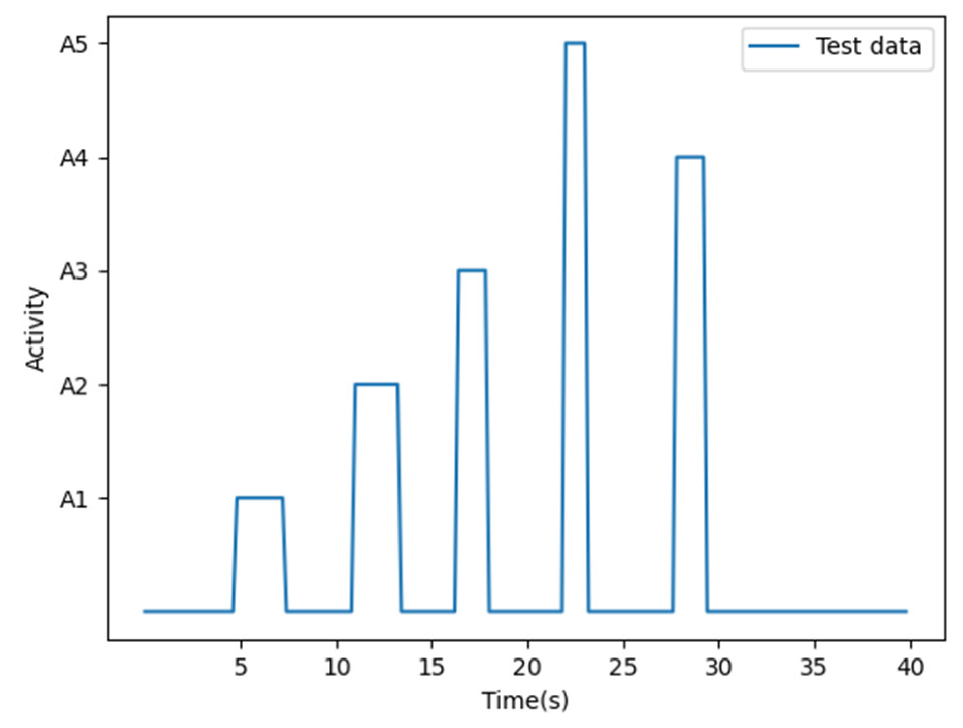
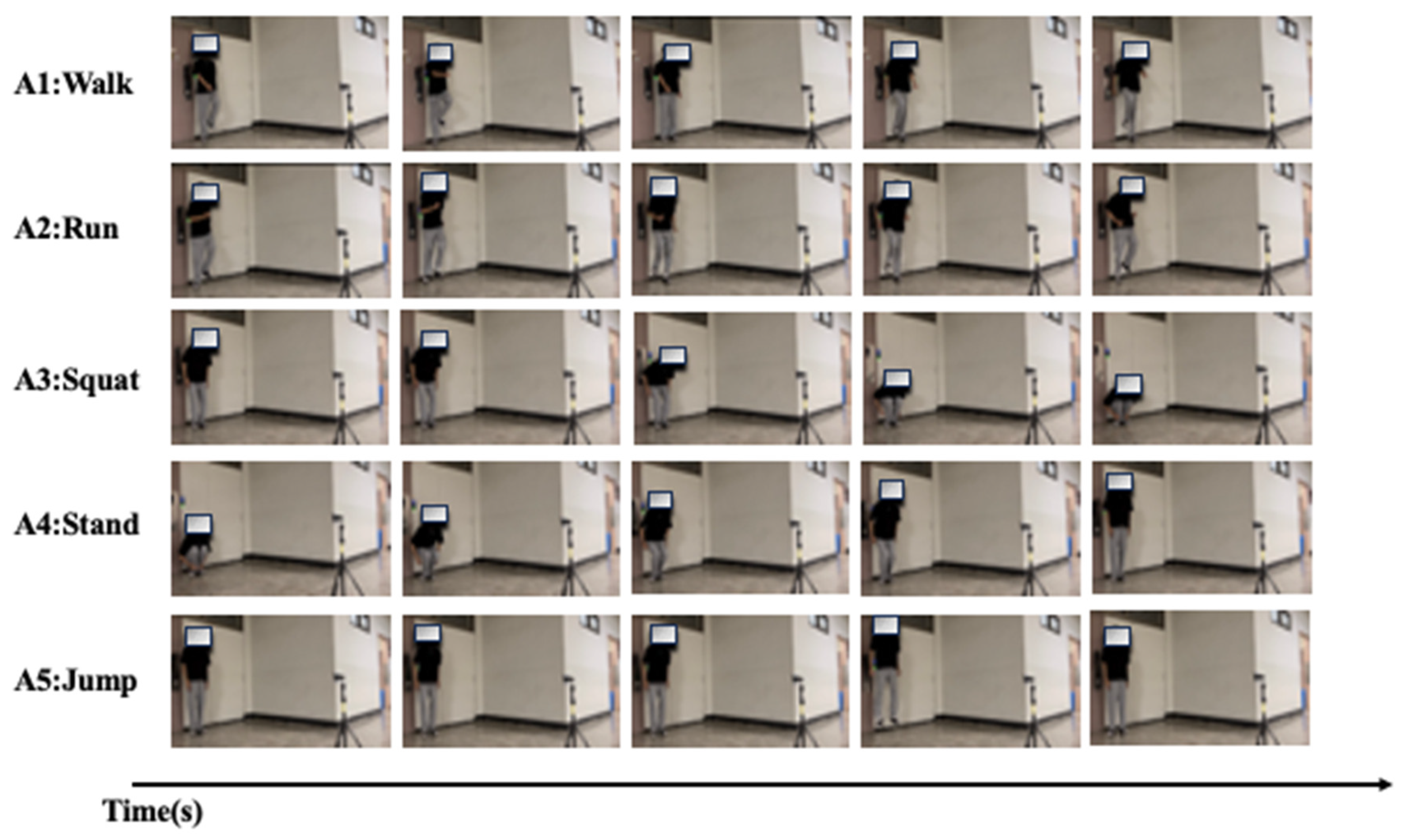
• We analyze realistic, continuous sequences of human activities rather than discrete activities. Within them, different actions can happen at any time, with unconstrained duration for each activity, and the body parts reposition themselves appropriately in order to perform the following activity.
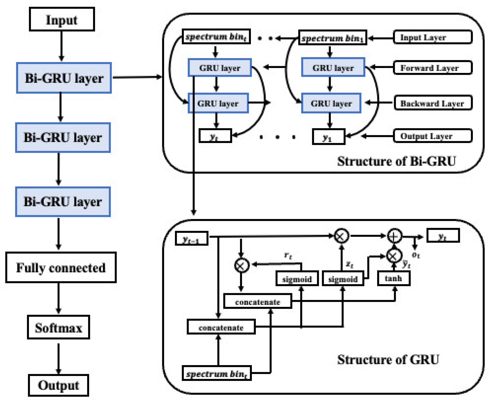
• We extract the Doppler feature from continuous-wave (CW) radar data. Then, we introduce stacked bidirectional GRU networks as a potent deep learning (DL) mechanism for classifying these ongoing human activity sequences. Bi-GRUs are inherently suitable for such analysis because they can capture both temporal forward and backward correlated information within the radar data. We also shed light on performance implications stemming from data-processing choices and pivotal hyperparameters.
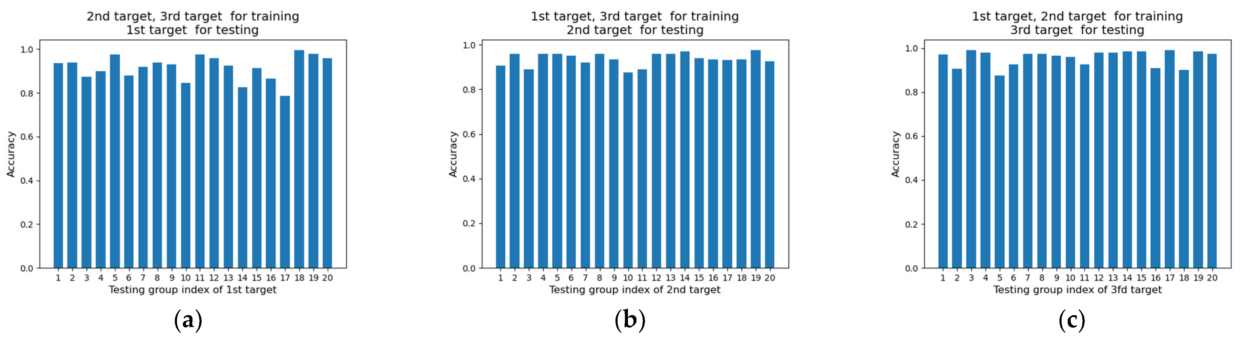
• We base our analysis on experimental data collected using a CW radar and involving three participants performing different combinations of five activities. Then, we design three different permutations, as shown in the table in Section 4.3, to train and test the model with different humans, which makes it more credible.

The remaining sections of this paper are organized as follows: Section 2 reviews the related works on human activity classification. Section 3 introduces the system description and main structure of the proposed radar-based Bi-GRU scheme. In Section 4, the performance of the proposed scheme is evaluated. Section 5 provides conclusions and discusses future works.

2. Related Works

Radar has been widely used in the field of human activity classification. The Bi-GRU is a lightweight neural network model, and it is usually suitable for small datasets, akin to our method. The authors in [25] proposed a deep learning (DL) method, called TRANS-Bi-GRU, which combines a transformer with a bidirectional gated recurrent unit (Bi-GRU) to efficiently learn and recognize different types of activities with a large dataset. They compared the proposed scheme with some existing schemes, and the results show that their scheme significantly outperforms the existing models for activity classification. However, this approach only used the raw data from the radar directly, without extracting the Doppler features from the raw data like our proposed scheme, which enables the fine-grained use of radar data. The authors in [13] proposed a robust fall detection system based on the frequency-modulated continuous-wave (FMCW) radar. The results show that the accuracy is over 90% on the test set. However, this scheme only detects the moment of human movement and calculates the range map of the radar signals, which cannot effectively utilize the data. On the other hand, the authors in [26] proposed an extremely efficient convolutional neural network (CNN) architecture named Mobile-RadarNet, specially designed for human activity classification based on micro-Doppler signatures. The experiments on a seven-class human activity dataset demonstrate that the proposed scheme can achieve high classification accuracy. Despite its high classification accuracy, it treats human activities as discrete, overlooking the continuous nature of most real-world activities. Our methodology, in contrast, treats continuous activities as a class, mirroring real-world scenarios more closely.

3. Proposed Bi-GRU Algorithm

3.1. System Description and Data Processing

The simplified overview of our proposed method for continuous human activity classification is illustrated in Figure 1. In the data acquisition part, the echo signals are recorded by a continuous wave (CW) radar. In the signal processing part, the fast Fourier transform (FFT) is employed to extract the Doppler features from the CW radar data, leading to time-Doppler spectra. In the activity classification part, the above time-Doppler spectra are fed into our proposed network, culminating in the final classification results.

The CW radar is the simplest and most efficient solution in cases where the detection of the moving object is the only, and outstanding, task [18,27]. Figure 2 shows the Doppler signature, capturing 40 s during which an individual cycles through five activities: walking, running, squatting, standing, and jumping. The y-axis in the figure denotes the Doppler dimension, while the x-axis highlights the time progression. Figure 2 distinctly showcases the varied Doppler signatures associated with different activities. For example, a negative frequency shift is observed when the participant squats, indicating movement away from the radar. Conversely, a positive frequency shift arises when the participant stands, symbolizing movement toward the radar.

Figure 3 elucidates the core steps of data processing. The captured signals manifest as a matrix structured by slow and fast time dimensions. Fast time refers to the time domain of individual pulse signals received by the radar; they are transformed into the fast time domain for the analysis and processing of each pulse signal. Slow time refers to the longer time scale in a radar system, involving a sequence of multiple pulse signals received over a period of time. The slow time domain is used to accumulate and integrate multiple pulse signals to improve the performance and target detection capability of the radar system. For data to be used as inputs to the classifier, firstly, a Fast Fourier transform is performed on each fast time bin of raw data to convert the time domain into a frequency domain to extract the information of the fast time dimension. To remove static clutter, a Hanning window is then applied, and then using specific slow time bins where the target is performing the activities, a 2D Fast Fourier transformation (FFT) is applied to find the Doppler-time pattern to characterize the micro-Doppler signatures. Each Doppler spectrum time bin is then manually labeled, setting the stage for model training. Figure 4 is the result after being given the label of Figure 2 (A1, A2, A3, A4 and A5 in the figure represent walking, running, squatting, standing, and jumping, respectively).

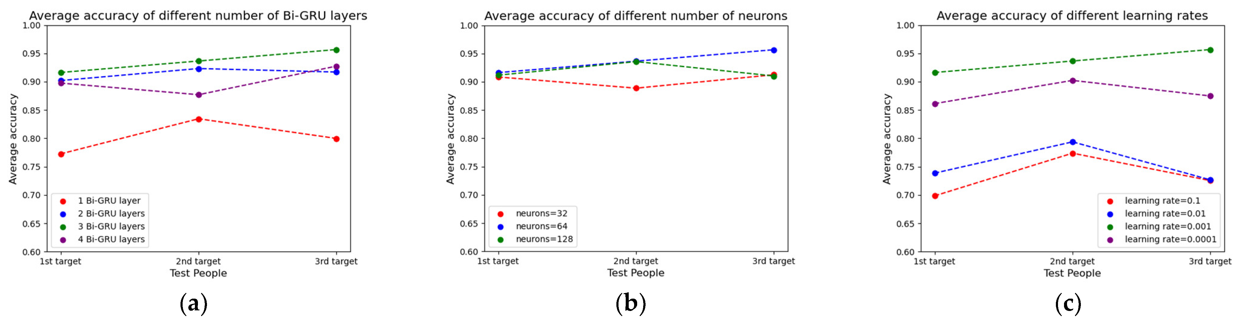
3.2. Optimal Parameters for Human Activity Classification

We implemented the neural network using a combination of software tools commonly employed in deep learning research. The primary components of our software stack included PyCharm version 2022.2.2 as the integrated development environment (IDE), Anaconda (Python version 3.9) for package management and environment control, and TensorFlow version 2.9.1 as the deep learning framework.

For many sequence modeling tasks, it is helpful to access future and post contexts. However, the standard GRU network processes the sequence in chronological order, ignoring the future context. Bi-GRU networks extend the unidirectional GRU network by introducing a second layer, in which the hidden connections flow in reverse chronological order. As a result, the model can take advantage of past and future information. The typical structure of GRU is shown in Figure 5. As mentioned earlier, GRU consists of an update and reset gate [1]. In the update gate, GRU computes ${\mathcal{z}}_t$ at a given time $t$ to solve the vanishing gradient problem using the following formula:

$${\mathcal{z}}_t=sigmoid\left(W_{\mathcal{z}}\left[y_{t-1},spectrum {bin}_t\right]\right).$$

(1)

${\mathcal{z}}_t$ is the output vector of the update gate, which controls the degree to which the previous hidden state $y_{t-1}$ influences the current input $spectrum {bin}_t$. Sigmoid is the activation function, $W_{\mathcal{z}}$ is the weight matrix, $y_{t-1}$ is the previous hidden state, and $spectrum {bin}_t$ is the current input GRU calculates $r_t$ at a given time $t$ to illustrate how much past information to forget. The gate executes the following formula:

$$r_t=sigmoid\left(W_r\left[y_{t-1}, spectrum {bin}_t \right]\right).$$

(2)

$r_t$ is the reset gate output vector, which determines how much of the previous hidden state $y_{t-1}$ should be ignored or reset based on the current input $spectrum {bin}_t$. $W_r$ is the weight matrix. The current storage content stage is calculated according to the following formula:

$${ \tilde{y}}_t=tanh\left(W_r\left[y_{t-1}, spectrum {bin}_t\right]\right).$$

(3)

${ \tilde{y}}_t$ is the new candidate hidden state, which is computed based on the previous hidden state $y_{t-1}$ and the current $spectrum {bin}_t$. tanh is the hyperbolic tangent activation function. Subsequently, the current hidden state, $y_t$, is computed based on the previous hidden state, current candidate activation, and update gate, using the equation

$$y_t=\left(1-{\mathcal{z}}_t\right)y_{t-1}+{\mathcal{z}}_t{ \tilde{y}}_t.$$

(4)

$$o_t=\left(W_0{y}_t\right).$$

(5)

$y_t$ is the current hidden state at time t, $y_{t-1}$ is the previous hidden state at time step $t-1$, $o_t$ is the output at time step, and $W_0$ is the weight matrix. For many sequence modeling tasks, it is helpful to access future and post contexts. However, the standard GRU network processes the sequence in chronological order, ignoring the future context. Bi-GRU networks extend the unidirectional GRU network by introducing a second layer, in which the hidden connections flow in reverse chronological order [28]. As a result, the model can take advantage of past and future information.

Figure 5 shows a simplified block diagram of the proposed architecture of the Bi-GRU network. The input to this network is the spectrogram, which contains micro-Doppler information and is fed into the network as a group of different vectors’ time bin after the time bin. Our Bi-GRU network is structured in a sequential manner, where the output layer of one Bi-GRU is connected to the input layer of the next Bi-GRU. This sequential connection enables the network to capture complex temporal dependencies within the data. Specifically, the hidden states of the first Bi-GRU layer serve as inputs to the second Bi-GRU, and so on for subsequent layers. This hierarchical architecture allows the network to learn and refine features at different levels of abstraction. In terms of training, we employed a holistic approach by training the entire stacked network from examples, as opposed to training each Bi-GRU layer separately. This comprehensive training strategy facilitates the learning of hierarchical representations from the data. Each layer of the network contributes to the extraction of relevant features, and the subsequent layers build upon these representations, ultimately leading to the high classification performance reported in our study. To estimate the influence of different hyper-parameters on the model performance, we will compare the average accuracy when the learning rate, the number of Bi-GRU layers, and the number of Bi-GRU neurons are different. We use two targets’ data to train the model and use the remaining one target’s data to test the model. The results are presented as follows.

(1) 

number of Bi-GRU layers

Figure 6a presents the average accuracies of the three targets in comparison with four distinct Bi-GRU layers: one layer, two layers, three layers, and four layers. All Bi-GRU parameters are set to be identical, except for the number of Bi-GRU layers. As can be observed, using three Bi-GRU layers results achieves the peak classification accuracy for all three target datasets, followed by the two Bi-GRU layers. The least average classification accuracy is found when using one Bi-GRU layer. In conclusion, the average classification accuracy improves when transitioning from one to three Bi-GRU layers. However, an increase to four Bi-GRU layers does not yield further gains. This plateau may arise from the model’s heightened complexity, which might lead to overfitting, meaning the model over-learns from the training data, capturing noise and unnecessary details. Therefore, the ability to generalize weakens, affecting the performance on test data. In the end, the number of Bi-GRU layers is set to three.

(2) 

number of Bi-GRU neurons

It is widely understood that amplifying the number of Bi-GRU neurons augments the model’s complexity, enabling it to capture more from the training data. However, an excessively intricate model might not necessarily perform well, especially if it over-learns, including noise and other irrelevant details, compromising the model’s generalization capability. Hence, a balanced, appropriate model is more beneficial than an overly complex model.

Figure 6b presents the average classification accuracies for three distinct Bi-GRU neuron counts: 32, 64, and 128. All other parameters remain consistent except for the neuron count. The optimal average classification accuracy emerges with 64 neurons, trailed by 128 neurons. The least effective configuration utilizes 32 neurons. Given these findings, the number of Bi-GRU neurons is set to 64.

(3) 

learning rate

The Adam optimizer is implemented for the model. A crucial hyperparameter to adjust in the update of the model parameters is the optimizer learning rate, often known as the step size. In this experiment, we conduct several tests to configure the optimal learning rate. Figure 6c illustrates the average classification accuracies of the three targets with four learning rates: ${10}^{-1}$, ${10}^{-2}$, ${10}^{-3}$, and ${10}^{-4}$. The figure shows that the highest average accuracies of the three targets all occur when learning rate is set to ${10}^{-3}$. To ensure the model functions optimally on our dataset, we apply a learning rate of ${10}^{-3}$.

4. Experiment and Results

4.1. Measurement Hardware and Its Parameters

The CW radar, supplied by the Innocent Company, works in a 24 GHz industrial, scientific, and medical (ISM) frequency. The radar sensor has only one transmitter channel and receiver channel. A summary of the technical details of our test apparatus is presented in

Table 1. Configuration parameters of CW radar.

Parameters	Values
Radar type	CW (1 − Tx and 1 − Rx)
CW Frequency	24,000 MHz
Sampling period	0.0004 s
Number of samples	128
Sampling time	0.0512 s
Velocity resolution	0.122 m/s
Low-pass filter (theoretical)	1250 Hz
Low-pass filter (current hardware)	915 Hz
High-pass filter (theoretical)	19.53 Hz
High-pass filter (current hardware)	20 Hz

.

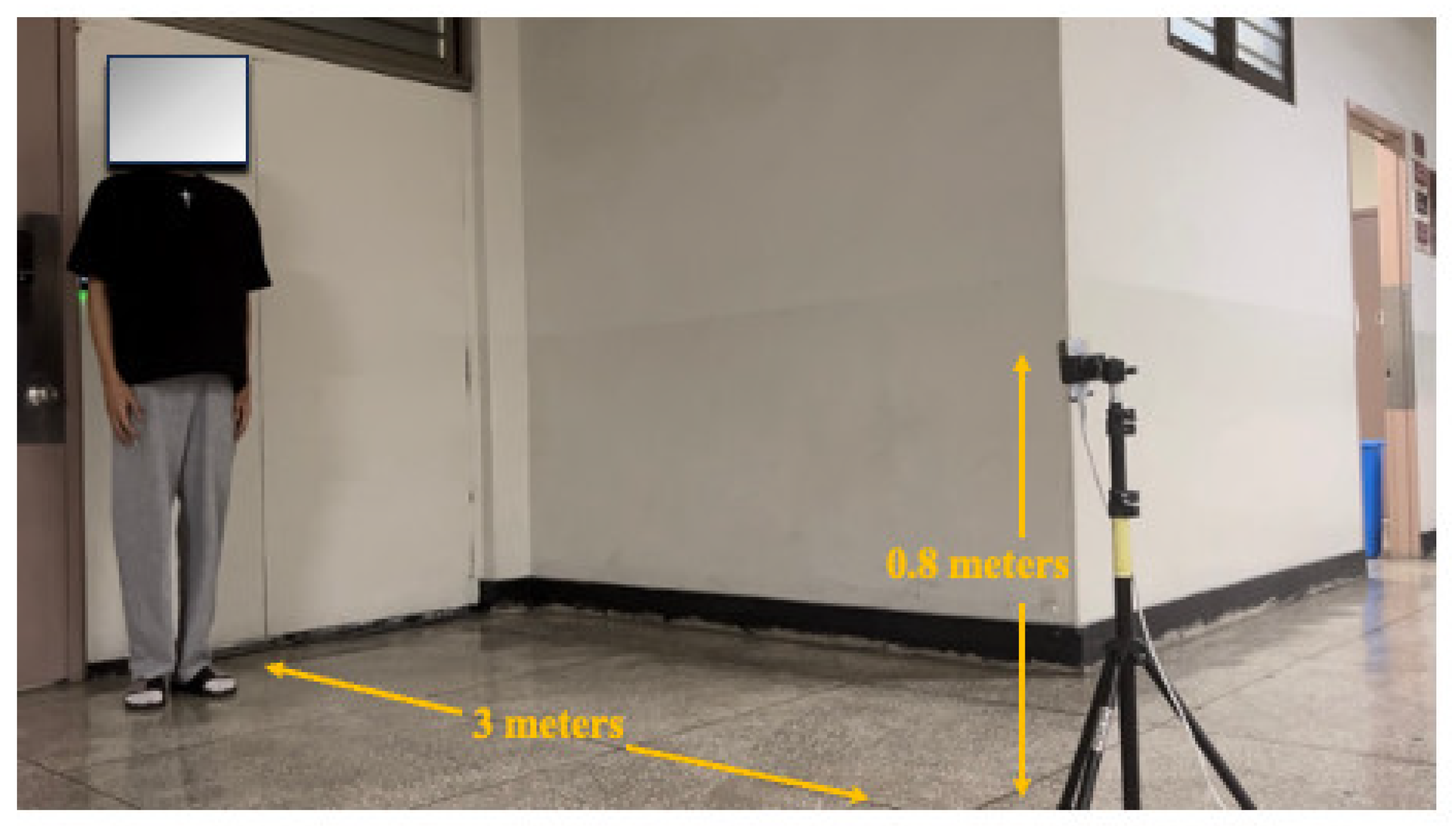
4.2. Experiment Scenario Setup and Data Collection

Data were collected from three participants, aged between 23 and 31, on the sixth floor of the Hwado Office Building at Kwangwoon University.

Table 2. Main physical parameters of participants.

No.	Gender	Age (yr)	Weight (kg)	Height (cm)
1	Man	26	81	177
2	Man	23	60	177
3	Man	31	72	170

provides the primary physical attributes of these participants. The radar was positioned at a height of 0.8 m, with a distance of 3 m from the participant. Figure 7 depicts the layout of the environment and radar setup.

Based on the purpose of detecting human activities in disasters, we designed several activities commonly used in disasters. The data include five human activities as shown in Figure 8: walk (A1), run (A2), squat (A3), stand (A4), and jump (A5). While each activity is presented as a distinct action, they were executed in a continuous sequence. Most research collects discrete activity. For example, the participant performs a single activity during one collection. However, we collected continuous activity. The participant performs five different activities continuously during one collection because activities in real-life scenarios tend to be continuous. Upon activating the radar, participants carried out all five activities in random order without constraints. Each data collection session lasted 40 s, during which participants completed all five activities. People can perform the five activities in a random order and the speed of the activity also depends on the participant. One important point is that the participant must perform all five activities in the 40s collection time, and each activity can only be performed one time. Such a session is termed a “group”, and every participant undertakes 20 groups. With three participants, this totaled 60 groups within a singular experimental setup. Each group was segmented into 200 bins, each lasting 0.2 s. Each bin was labeled according to the activity conducted during that time. Subsequently, these bins were inputted into the model group by group.

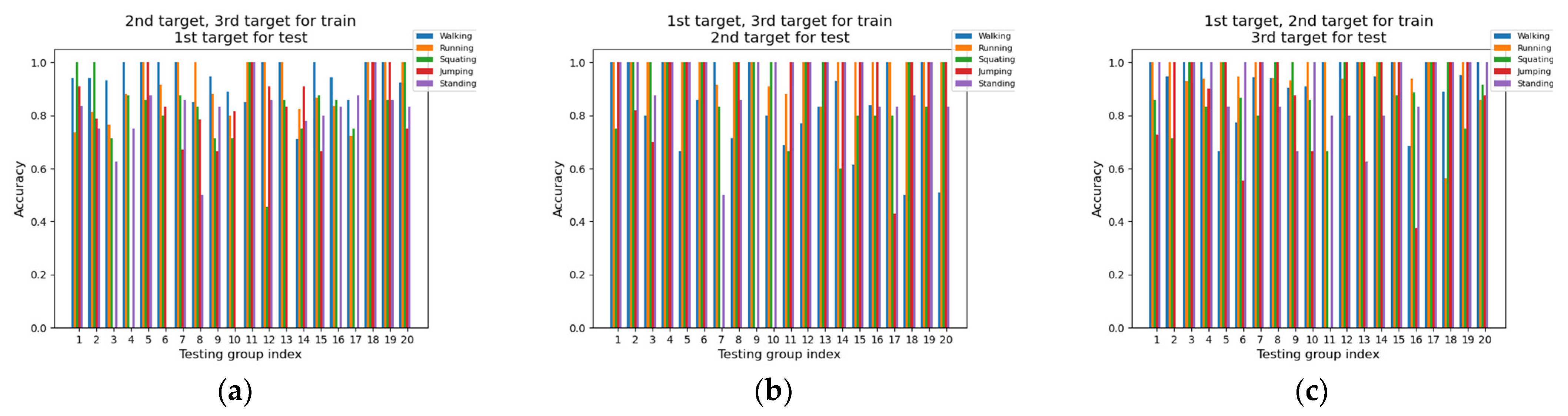
4.3. Training and Testing Set Composition

Sixty distinct groups were gathered in total. To bolster the credibility of our results, data from two targets (or 40 groups) were used for training, while data from the third target (20 groups) were allocated for testing.

Table 3. All permutations of the train and test sets.

No.	Train Set	Test Set
1	2nd target, 3rd target	1st target
2	1st target, 3rd target	2nd target
3	1st target, 2nd target	3rd target

lists all the permutation combinations considered. The target we mentioned in Table 3 refers to the participant in our experiment.

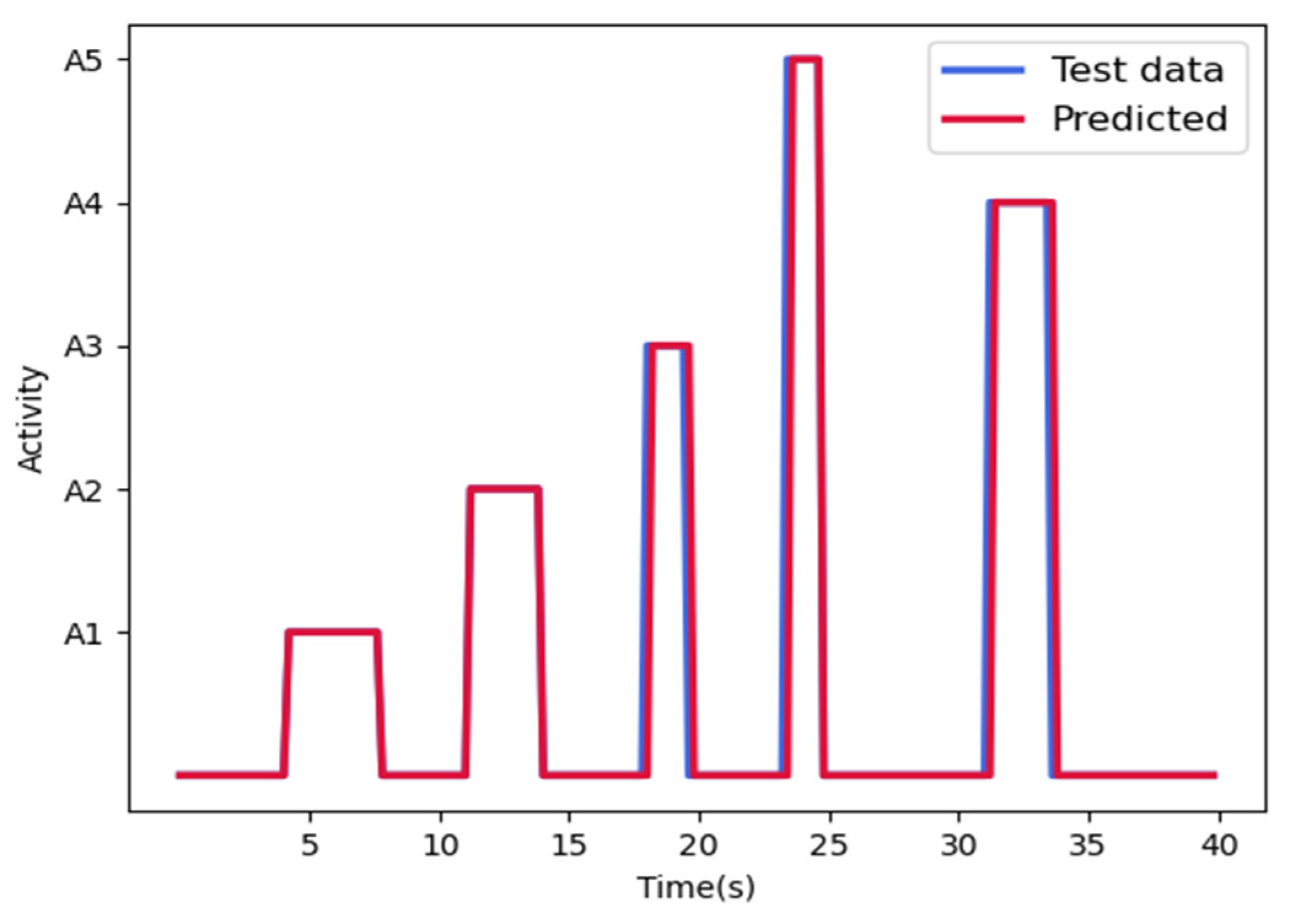
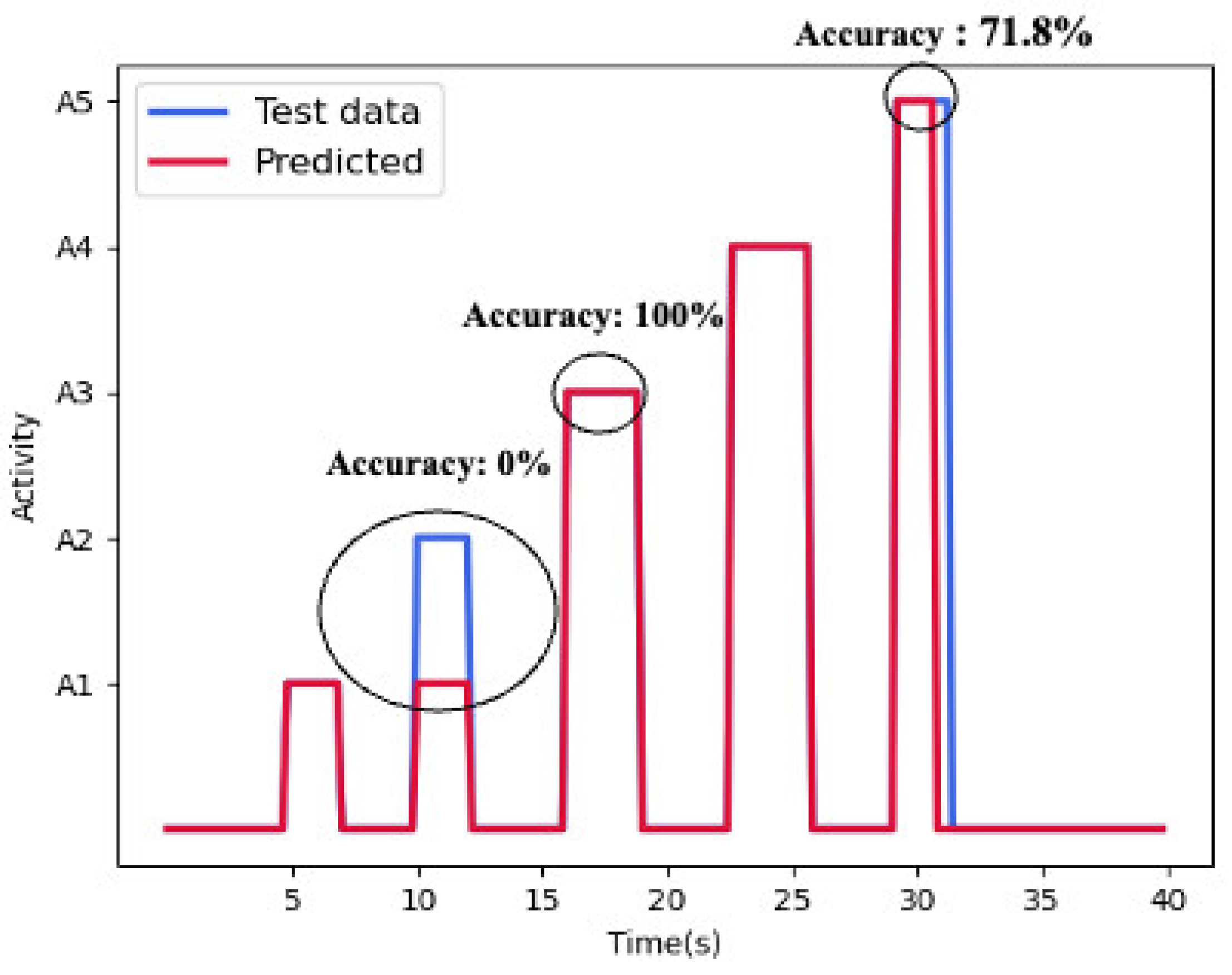
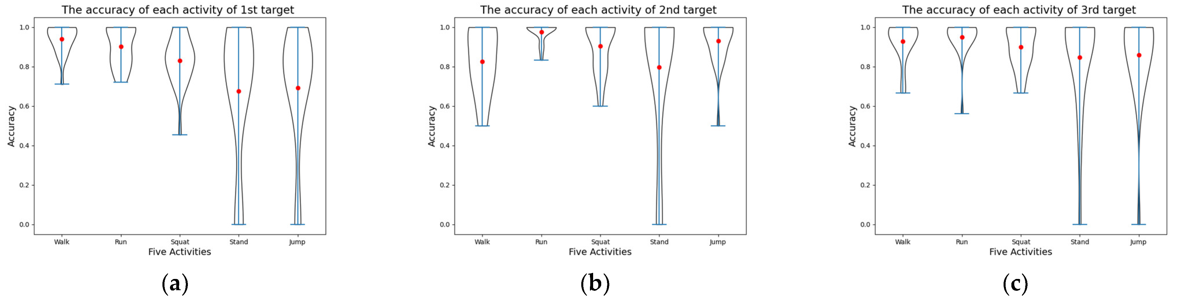
4.4. Performance Analysis

Figure 9 shows an example result of a group; the blue line is the actual activity of the participant, and the red line is the participant’s activity that the model predicts. The accuracy of the group is determined by comparing the blue line and the orange line. The accuracy of each activity is determined by comparing the blue line and orange line in each activity in the group. Many papers use the data of the same target to train and test. However, when they use the same target’s data to train and test, this means that the model already learns the feature of the test target. Therefore, it cannot show that the model has a good generalization ability. In our experiment, we use different targets to train and test to let the results be more persuasive.

Figure 10 shows the accuracy of each group when we use two targets’ data to train the model and use the remaining one target’s data to test the model. It is obviously shown in Figure 10 that many accuracy rates exceed 95% and most accuracy rates exceed 90%, especially in Figure 10b,c. However, not all test groups maintain this high level of accuracy due to the inherent challenges of detecting intricately designed activities within this dataset. For instance, the 17th group in Figure 10a has an accuracy of approximately 78%. This variability can be attributed to the fact that the same activity, when performed by the same target, might exhibit slight differences across different targets. Consequently, Doppler features might vary between participants, leading to occasional inconsistencies in the model’s predictions.

Beyond group-wise accuracy, we also evaluated the accuracy for each distinct activity within every group to verify the experiment’s authenticity. Figure 11 shows an example about how to calculate the accuracy of each activity. On the one hand, the model sometimes cannot predict the correct activity like the first circle on the figure, which results in 0% accuracy; on the other hand, the model can sometimes predict the correct activity but cannot predict the duration of the activity correctly, such as the third circle on the figure, which results in 71.8% accuracy. In the next section, we will introduce the results of the accuracy of each activity in every group.

Figure 12 presents the accuracy of individual activities across groups, using two targets’ data for training and the remaining one target’s data for testing. From Figure 12, we can see that the best result is Figure 12c, followed by Figure 12b, and most of the accuracies in both are over 90%. Then, there is Figure 12a, in which most of the accuracies are over 80%. From Figure 10 and Figure 12, we can see that the model behaves well when using the data of the second target and third target to test, and the model behaves less well when the data of the first were used for testing.

Figure 13 illustrates a violin plot of the accuracy for five distinct activities across different targets. The mean accuracies for the activities walk and run consistently surpass 95%, except for the walk activity in Figure 13b. This high accuracy can be attributed to the extended duration of walking and running relative to other activities, allowing the model to glean more characteristic features from these two activities. In contrast, the average accuracies for the squat activity are approximately 90% in Figure 13b,c but drop to approximately 80% in Figure 13a. The jump and stand activities yield mean accuracies of approximately 85% in Figure 13b,c. However, these values significantly dip to approximately 65% in Figure 13a. One potential explanation is the inherent variability in the way different targets perform the same activity, leading to inconsistent accuracy when different targets’ data are used for training and testing, as observed in the jump and stand activities within Figure 13a.

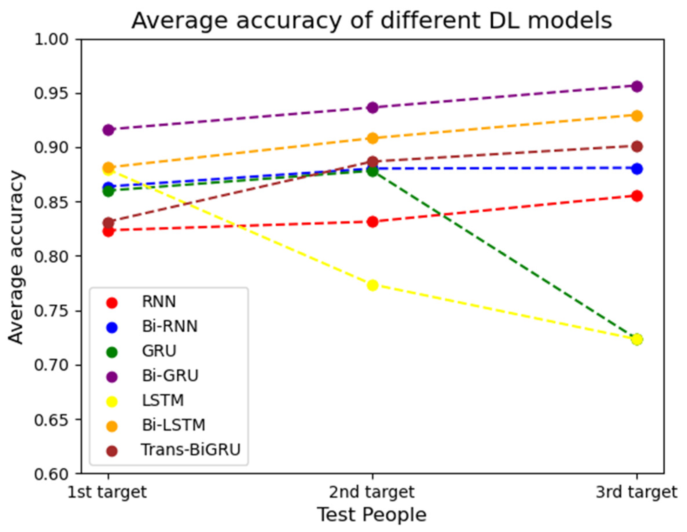
4.5. Performance Comparison

To evaluate the performance of the proposed scheme, we compared the average accuracy of the group for the three participants with different deep learning models, as shown in Figure 14. As the figure indicates, the Bi-GRU approach consistently achieves average accuracies exceeding 0.9 for all participants, succeeded by the Bi-LSTM model, which yields average accuracies over 0.9 for the second and third targets. The worst is the LSTM scheme, in which the average accuracy for first target is approximately 0.88, the accuracy for the second target is approximately 0.77, and the accuracy for the third target is only approximately 0.72. Conversely, the Bi-GRU scheme achieves the best performance.

5. Conclusions and Future Work

This paper introduces a Bi-GRU model geared toward continuous human activity classification, leveraging the Doppler feature extracted from CW radar data. Our emphasis is on continuous human activities, as opposed to discrete ones, given the inherently continuous nature of real-world human actions. Going forward, we aspire to achieve real-time continuous human activity classification, fostering applications such as monitoring human activities during emergencies or disasters.

References

1. Shrestha, A.; Li, H.; Le Kernec, J.; Fioranelli, F. Continuous human activity classification from FMCW radar with Bi-LSTM networks. IEEE Sens. J. 2020, 20, 13607–13619. [Google Scholar] [CrossRef]
2. Khatun, M.A.; Yousuf, M.A.; Ahmed, S.; Uddin, M.Z.; Alyami, S.A.; Al-Ashhab, S.; Akhdar, H.F.; Khan, A.; Azad, A.; Moni, M.A. Deep CNN-LSTM with self-attention model for human activity recognition using wearable sensor. IEEE J. Transl. Eng. Health Med. 2022, 10, 2700316. [Google Scholar] [CrossRef] [PubMed]
3. Tong, L.; Ma, H.; Lin, Q.; He, J.; Peng, L. A novel deep learning Bi-GRU-I model for real-time human activity recognition using inertial sensors. IEEE Sens. J. 2022, 22, 6164–6174. [Google Scholar] [CrossRef]
4. Luo, F.; Khan, S.; Huang, Y.; Wu, K. Binarized neural network for edge intelligence of sensor-based human activity recognition. IEEE Trans. Mob. Comput. 2023, 22, 1356–1368. [Google Scholar] [CrossRef]
5. Teng, Q.; Tang, Y.; Hu, G. RepHAR: Decoupling networks with accuracy-speed tradeoff for sensor-based human activity recognition. IEEE Trans. Instrum. Meas. 2023, 72, 2505111. [Google Scholar] [CrossRef]
6. Xu, S.; Zhang, L.; Huang, W.; Wu, H.; Song, A. Deformable convolutional networks for multimodal human activity recognition using wearable sensors. IEEE Trans. Instrum. 2022, 71, 2505414. [Google Scholar] [CrossRef]
7. Imran, H.A. UltaNet: An Antithesis Neural Network for Recognizing Human Activity Using Inertial Sensors Signals. IEEE Sens. Lett. 2022, 6, 7000304. [Google Scholar] [CrossRef]
8. Rezaei, A.; Stevens, M.C.; Argha, A.; Mascheroni, A.; Puiatti, A.; Lovell, N.H. An unobtrusive human activity recognition system using low resolution thermal sensors, machine and deep learning. IEEE Trans. Biomed. Eng. 2023, 70, 115–124. [Google Scholar] [CrossRef]
9. Manaf, A.; Singh, S. Computer vision-based survey on human activity recognition system, challenges and applications. In Proceedings of the 2021 3rd International Conference on Signal Processing and Communication (ICPSC), Coimbatore, India, 13–14 May 2021; pp. 110–114. [Google Scholar]
10. Siddiqi, M.H.; Almashfi, N.; Ali, A.; Alruwaili, M.; Alhwaiti, Y.; Alanazi, S.; Kamruzzaman, M.M. A unified approach for patient activity recognition in healthcare using depth camera. IEEE Access 2021, 9, 92300–92317. [Google Scholar] [CrossRef]
11. Wang, B.; Zhang, H.; Guo, Y.-X. Radar-based soft fall detection using pattern contour vector. IEEE Internet Things J. 2023, 10, 2519–2527. [Google Scholar] [CrossRef]
12. Yu, Z.; Zahid, A.; Taha, A.; Taylor, W.; Kernec, J.K.; Heidari, H.; Ali, M.; Abbasi, Q.H. An intelligent implementation of multi-sensing data fusion with neuromorphic computing for human activity recognition. IEEE Internet Things J. 2023, 10, 1124–1133. [Google Scholar] [CrossRef]
13. Yao, Y.; Liu, C.; Zhang, H.; Yan, B.; Jian, P.; Wang, P.; Du, L.; Chen, X.; Han, B.; Fang, Z. Fall detection system using millimeter-wave radar based on neural network and information fusion. IEEE Internet Things J. 2022, 21, 21038–21050. [Google Scholar] [CrossRef]
14. Liu, Z.; Wu, C.; Ye, W. Category-extensible human activity recognition based on Doppler radar by few-shot learning. IEEE Sens. J. 2022, 22, 21952–21960. [Google Scholar] [CrossRef]
15. Abdu, F.J.; Zhang, Y.; Deng, Z. Activity classification based on feature fusion of FMCW radar human motion micro-doppler signatures. IEEE Sens. J. 2022, 22, 8648–8662. [Google Scholar] [CrossRef]
16. Vandersmissen, B.; Knudde, N.; Jalalvand, A.; Couckuyt, I.; Bourdoux, A.; Neve, W.D.; Dhaene, T. Indoor person identification using a low-power FMCW radar. IEEE Trans. Geosci. Remote Sens. 2018, 56, 3941–3952. [Google Scholar] [CrossRef]
17. Chen, V.C.; Li, F.; Ho, S.S.; Wechsler, H. Micro-Doppler effect in radar: Phenomenon, model, and simulation study. IEEE Trans. Aerosp. Electron. Syst. 2006, 42, 2–21. [Google Scholar] [CrossRef]
18. Chakraborty, M.; Kumawat, H.C.; Dhavale, S.V. DIAT-RadHARNet: A lightweight DCNN for radar-based classification of human suspicious activities. IEEE Trans. Instrum. Meas. 2022, 71, 2505210. [Google Scholar] [CrossRef]
19. Alnujaim, I.; Oh, D.; Kim, Y. Generative adversarial networks for classification of micro-doppler signatures of human activity. IEEE Geosci. Remote Sens. Lett. 2019, 17, 396–400. [Google Scholar] [CrossRef]
20. Chen, W.; Zhai, C.; Wang, X.; Li, J.; Lv, P.; Liu, C. GCN- and GRU-based intelligent model for temperature prediction of local heating surfaces. IEEE Trans. Ind. Inform. 2023, 19, 5517–5529. [Google Scholar] [CrossRef]
21. Shu, W.; Cai, K.; Xiong, N.N. A short-term traffic flow prediction model based on an improved gate recurrent unit neural network. IEEE Trans. Intell. Transp. Syst. 2022, 23, 16654–16665. [Google Scholar] [CrossRef]
22. Aslam, N.; Rustam, F.; Lee, E.; Washington, P.B.; Ashraf, I. Sentiment analysis and emotion detection on cryptocurrency related tweets using ensemble LSTM-GRU model. IEEE Access 2022, 10, 39313–39324. [Google Scholar] [CrossRef]
23. Xia, M.; Shao, H.; Ma, X.; de Silva, C.W. A stacked GRU-RNN-based approach for predicting renewable energy and electricity load for smart grid operation. IEEE Trans. Ind. Inform. 2021, 17, 7050–7059. [Google Scholar] [CrossRef]
24. Li, K.; Shen, N.; Kang, Y.; Chen, H.; Wang, Y.; He, S. Livestock product price forecasting method based on heterogeneous GRU neural network and energy decomposition. IEEE Access 2021, 9, 158322–158330. [Google Scholar] [CrossRef]
25. Chen, D.; Yongchareon, S.; Lai, E.; Yu, J.; Sheng, Q.; Li, Y. Transformer with bidirectional GRU for nonintrusive, sensor-based activity recognition in a multiresident environment. IEEE Internet Things J. 2022, 9, 23716–23727. [Google Scholar] [CrossRef]
26. Zhu, J.; Lou, X.; Ye, W. Lightweight deep learning model in mobile-edge computing for radar-based human activity recognition. IEEE Internet Things J. 2021, 8, 12350–12359. [Google Scholar] [CrossRef]
27. Yang, S.; Kim, Y. Single 24-GHz FMCW radar-based indoor device-free human localization and posture sensing with CNN. IEEE Sens. 2023, 23, 3059–3068. [Google Scholar] [CrossRef]
28. Xu, C.; Zhou, Y.; Wang, Q.; Ma, Z.; Zhu, Y. Detecting hypernymy relations between medical compound entities using a hybrid-attention based Bi-GRU-CapsNet model. IEEE Access 2019, 7, 175693–175702. [Google Scholar] [CrossRef]
Figure 1. The framework of the proposed Doppler-based Bi-GRU method.
Electronics 12 04060 g001
Figure 2. Doppler signature of a group.
Electronics 12 04060 g002
Figure 3. The main process of the data processing.
Electronics 12 04060 g003
Figure 4. The result after the data processing of Figure 2.
Electronics 12 04060 g004
Figure 5. The structure of the proposed Bi-GRU network.
Electronics 12 04060 g005
Figure 6. The average accuracy of using two targets’ data to train and using the remaining one target’s data to test with different model parameters: (a) various Bi-GRU layers, (b) various neurons, (c) various learning rates.
Electronics 12 04060 g006
Figure 7. Experiment environment.
Electronics 12 04060 g007
Figure 8. Pictorial list of activities; these five activities were performed in random continuous sequences.
Electronics 12 04060 g008
Figure 9. Ground truth in blue, and the predicted outcome in red.
Electronics 12 04060 g009
Figure 10. The accuracy of each group when we use two targets’ data to train and use the remaining one target’s data to test: (a) use the data of 2nd target and 3rd target to train, and use the data of 1st target to test; (b) use the data of 1st target and 3rd target to train, and use the data of 2nd target to test; (c) use the data of 1st target and 2nd target to train, and use the data of 3rd target to test.
Electronics 12 04060 g010
Figure 11. Example of how to calculate the accuracy of each activity.
Electronics 12 04060 g011
Figure 12. Accuracy of each activity in each group when we use two targets’ data to train and use the remaining one target’s data to test: (a) use the data of 2nd target and 3rd target to train, and use the data of 1st target to test; (b) use the data of 1st target and 3rd target to train, and use the data of 2nd target to test; (c) use the data of 1st target and 2nd target to train, and use the data of 3rd target to test target to test.
Electronics 12 04060 g012
Figure 13. Violin plot of the accuracy of five activities for different targets: (a) use the data of 2nd target and 3rd target to train, and use the data of 1st target to test; (b) use the data of 1st target and 3rd target to train, and use the data of 2nd target to test; (c) use the data of 1st target and 2nd target to train, and use the data of 3rd target to test.
Electronics 12 04060 g013
Figure 14. Average accuracy of the three targets when using different models.
Electronics 12 04060 g014