Enhanced Grey Wolf Optimization Algorithm for Mobile Robot Path Planning

Abstract

In this study, an enhanced hybrid Grey Wolf Optimization algorithm (HI-GWO) is proposed to address the challenges encountered in traditional swarm intelligence algorithms for mobile robot path planning. These challenges include low convergence accuracy, slow iteration speed, and vulnerability to local optima. The HI-GWO algorithm introduces several key improvements to overcome these limitations and enhance performance. To enhance the population diversity and improve the initialization process, Gauss chaotic mapping is applied to generate the initial population. A novel nonlinear convergence factor is designed to strike a balance between global exploration and local exploitation capabilities. This factor enables the algorithm to effectively explore the solution space while exploiting the promising regions to refine the search. Furthermore, an adaptive position update strategy is developed by combining Levy flight and golden sine. This strategy enhances the algorithm’s solution accuracy, global search capability, and search speed. Levy flight allows longer jumps to explore distant regions, while golden sine guides the search towards the most promising areas. Extensive simulations on 16 standard benchmark functions demonstrate the effectiveness of the proposed HI-GWO algorithm. The results indicate that the HI-GWO algorithm outperforms other state-of-the-art intelligent algorithms in terms of optimization performance. Moreover, the performance of the HI-GWO algorithm is evaluated in a real-world path planning experiment, where a comparison with the traditional grey wolf algorithm and ant colony algorithm validates the superior efficiency of the improved algorithm. It exhibits excellent optimization ability, robust global search capability, high convergence accuracy, and enhanced robustness in diverse and complex scenarios. The proposed HI-GWO algorithm contributes to advancing the field of mobile robot path planning by providing a more effective and efficient optimization approach. Its improvements in convergence accuracy, iteration speed, and robustness make it a promising choice for various practical applications.

1. Introduction

Mobile robot path planning has become a crucial research area in the field of robotics due to its wide range of applications in various domains, including autonomous navigation, industrial automation, and search and rescue operations [1,2]. The ability to plan an optimal path for a mobile robot is of utmost importance as it directly impacts the efficiency and safety of the robot’s operation. The task of mobile robot path planning involves determining a collision-free trajectory from a starting point to a goal point while avoiding obstacles in the environment. This seemingly simple objective poses significant challenges due to several factors [3,4]. First, static obstacles in the environment pose challenges as they need to be identified and avoided effectively. These obstacles can vary in shape, size, and distribution, making it difficult to devise efficient algorithms that can handle diverse scenarios. Second, the path planning problem is computationally demanding, especially when dealing with large-scale environments. Real-time performance is essential for practical applications, and finding an optimal path within a reasonable time frame is critical. Finally, the presence of uncertainty, such as sensor noise or imperfect information about the environment, further complicates the path planning task. Existing path planning methods include traditional algorithms like Dijkstra’s algorithm, artificial potential field method, A* algorithm [5], and intelligent algorithms like ant colony algorithm and genetic algorithm [6]. Additionally, novel bio-inspired swarm intelligence algorithms, such as the whale optimization algorithm and the bat algorithm, have been developed, along with combinations of these algorithms. For instance, Selcuk et al. (2023) applied the Immune Plasma algorithm to solve the path planning problem for unmanned combat aerial vehicles (UCAVs). They investigated its capabilities by assigning different values to the population size and number of donor–receivers and using challenging battlefield scenarios. The results obtained by the Immune Plasma algorithm were compared with those of well-known meta-heuristic algorithms. The comparative studies revealed that the Immune Plasma algorithm is capable of finding more robust paths for UCAVs operating on battlefields, outperforming other executed algorithms in most test scenarios [7]. To address the complexity of path planning in complex environments for unmanned aerial vehicles (UAVs), Ma et al. (2022) proposed an adaptive path planning method based on discrete global grid systems. This method incorporates conflict detection between airspace and UAV paths. The proposed method was validated through comparison with other particle swarm optimization (PSO) algorithms and simulation-based experiments, illustrating its optimality [8]. Vincent et al. (2022) considered fixed-wing autonomous UAVs in complex 3D environments and used a non-deterministic Flower Pollination Algorithm (FPA) to compute feasible and quasi-optimal trajectories. They improved the global optimization algorithm by adding a deterministic 2-opt local search, resulting in significant improvements. The proposed trajectory planner was implemented and parallelized on a Graphics Processing Unit (GPU) using the Compute Unified Device Architecture (CUDA), achieving a speedup of 253.4× compared to the sequential implementation on a CPU. The parallel implementation can compute quasi-optimal trajectories in just 0.369 s [9]. To enhance traditional Genetic Algorithms for path planning in specific application scenarios, Wei et al. (2021) proposed a new path planning algorithm for mobile robots. They added path smoothness and the number of path corners to the fitness function for evaluating the path, aiming to select a superior one. MATLAB simulation experiments demonstrated the validity and feasibility of the modified method. Compared to traditional Genetic Algorithms and other classical path planning algorithms, the optimal path selected had fewer turning angles under the same path length. This improved application efficiency and stability [10]. Drawing inspiration from natural flow patterns that avoid rocks, Yao et al. (2018) developed a submerged path planning method based on an improved interfered fluid dynamical system (IIFDS). They applied a reverse-avoidance strategy to real-time path planning to circumvent dynamic obstacles combined with IIFDS. Simulation results from various scenarios verified the favorable performance of their proposed method [11]. For solving UAV path planning problems in a 3D environment, Chen et al. (2023) proposed an enhanced version of the Chimp Optimization Algorithm (TRS-ChOA). Through testing on benchmark functions and CEC2017 complex functions, TRS-ChOA demonstrated superior optimization capability and robustness compared to other algorithms. The researchers applied TRS-ChOA alongside five well-known algorithms to solve path planning problems in three 3D environments. Experimental results revealed that TRS-ChOA reduced the average path length/fitness value by a significant percentage compared to other algorithms, indicating that the flight paths planned by TRS-ChOA were more cost-effective, smoother, and safer [12]. Wang et al. (2022) transformed the UAV route planning issue into an optimization problem that meets the UAV’s feasible path requirements and safety constraints. They introduced a modified Mayfly Algorithm (modMA) incorporating an exponent decreasing inertia weight (EDIW) strategy, adaptive Cauchy mutation, and an enhanced crossover operator to effectively search the UAV configuration space and discover the path with the lowest overall cost. The proposed modMA was evaluated on benchmark functions as well as the UAV route planning problem, outperforming the other compared algorithms [13]. To address security attacks such as denial-of-service (DoS) and Man-in-the-Middle (MITM) attacks and achieve secure path planning for UAVs, Kayalvizhi et al. (2022) proposed a novel Resilient UAV Path Optimization Algorithm (RUPOA). This algorithm was compared with existing path planning algorithms based on execution time. To mitigate security attacks, they also proposed a blockchain-aided security solution. They utilized smart contracts to register devices with gasLimit, preventing security attacks. The performance efficiency of the blockchain model was evaluated based on network latency, which represents the total execution time across the blockchain network [14]. To overcome the increased computation time of UAV path planning problems in dynamic 3D environments, Raja et al. (2022) introduced a new parallel multiobjective multiverse optimizer (PMOMVO). They successfully applied this algorithm and carried out demonstrative results and nonparametric ANOVA statistical analyses. These analyses showcased the effectiveness and superiority of the proposed PMOMVO algorithm compared to other homologous multiobjective metaheuristics [15]. In order to find shorter and more stable paths, Zheng et al. (2023) proposed an improved version of the SMA called the Levy flight-rotation SMA (LRSMA). LRSMA utilizes a variable neighborhood Levy flight and an individual rotation perturbation and variation mechanism to enhance local optimization ability and avoid falling into local optima. Experiments conducted in varying environments demonstrated that the proposed algorithm can generate collision-free paths with the shortest length, higher accuracy, and robust stability [16].

However, each algorithm has its limitations. Among them, the GWO algorithm is a novel bio-inspired swarm intelligence optimization algorithm that was proposed by Mirjalili et al. in 2014. It solves problems by simulating the hunting behavior of grey wolf populations in the biological world. GWO has gained popularity due to its advantages, such as having fewer adjustable parameters, ease of implementation, and high efficiency compared to other intelligent algorithms [17]. Consequently, it has been widely applied to optimization problems, scheduling problems, and system configuration [18]. Mobile robot path planning is a significant challenge due to the intricate and dynamic nature of the environments in which robots navigate. The objective is to find an optimal or near-optimal path while considering obstacles and constraints. Existing approaches, such as the standard GWO algorithm, have limitations that hinder their effectiveness in this task. The GWO algorithm suffers from several drawbacks that restrict its performance in robot path planning. One limitation is its inflexible search strategies, which limit the exploration of the solution space and hinder the algorithm’s ability to find optimal paths in complex environments. Additionally, the slow convergence speed during later stages of optimization reduces its efficiency for real-time path planning scenarios. Moreover, the GWO algorithm is prone to getting trapped in local optima, resulting in suboptimal or inefficient paths for mobile robots.

To address these limitations, we propose the hybrid improved Grey Wolf Algorithm (HI-GWO), which integrates additional optimization techniques and modifications. In addition to concepts such as Levy flight and the golden sinusoidal function, we further enhance HI-GWO by incorporating a nonlinear convergence factor and Gauss chaotic mapping. By introducing the nonlinear convergence factor and Gauss chaotic mapping, HI-GWO addresses the GWO algorithm’s limitations. The nonlinear convergence factor dynamically adjusts the balance between exploration and exploitation, improving the convergence speed and solution quality. It allows HI-GWO to adaptively explore the solution space, thoroughly searching for optimal paths in complex environments while avoiding trapping in local optima. Furthermore, the integration of Levy flight and the golden sinusoidal function enhances the search capabilities of HI-GWO. Levy flight introduces randomness into the search process, enabling larger jumps and exploration of distant regions in the solution space. This helps the algorithm escape local optima and enhances its global search capability. The golden sinusoidal function guides the algorithm towards promising areas while still exploring other regions, promoting the identification of more optimal paths for mobile robots.

To evaluate the performance of HI-GWO, extensive experimentation and comparative analysis with existing optimization algorithms will be conducted. The convergence speed, solution quality, scalability metrics, and other relevant measures will be utilized to demonstrate the superiority of HI-GWO over other state-of-the-art approaches. Through this research, our aim is to advance the theoretical understanding of the GWO algorithm and provide practitioners with an advanced optimization tool specifically tailored to the requirements of mobile robot path planning tasks. By integrating the nonlinear convergence factor, Gauss chaotic mapping, Levy flight, and the golden sinusoidal function, we overcome limitations in search strategies, convergence speed, and local optima trapping. This results in improved performance and efficiency in finding optimal paths for mobile robots in complex environments.

The article is structured as follows: Section 1 provides an introduction to the research topic, while Section 2 presents the methods used, including the GWO algorithm and the HI-GWO algorithm with its various components. In Section 2, the specific implementation steps and details of the problem-solving method are discussed. Section 3 focuses on the results obtained from different experiments and mobile robot path planning simulations. Finally, Section 4 draws conclusions based on the findings and outlines future research directions.

2. Methods

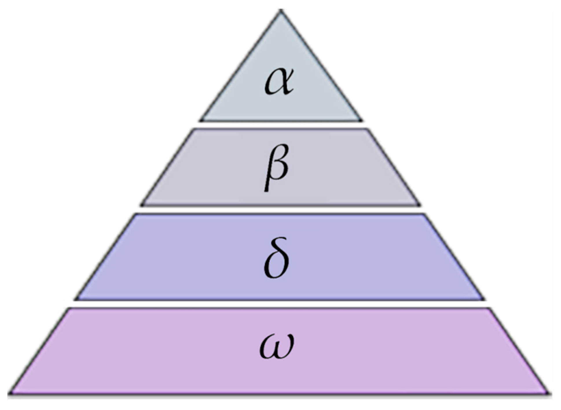
2.1. Grey Wolf Optimization (GWO) Algorithm

Studies have revealed that grey wolves, which fall under the category of canids, hold a prominent position at the apex of the ecological food chain, earning them the distinction of being top-level predators. It has been observed that these animals exhibit a marked inclination towards group living, displaying an intricate social order within their packs, as illustrated in Figure 1. At the highest tier of this hierarchical structure stands the α wolf, who assumes the role of the pack’s leader, wielding the responsibility of managing the group dynamics and making crucial decisions. Just below that, we find the β wolves tasked with supporting the alpha wolf and prepared to step up if a leadership position becomes vacant. Occupying the third level are the δ wolves, obediently following the orders issued by the leaders above while fulfilling duties such as surveillance and reconnaissance. Lastly, positioned at the bottom tier, we find the ω wolves, whose primary role revolves around maintaining harmonious relations within the population [19,20].

A single iteration of the GWO algorithm consists of four main processes: hierarchy division, searching, encircling, and attacking. Firstly, the wolf population is hierarchically divided based on the fitness of individual members, labeled as, α, β, δ, and ω. The optimization process of the algorithm primarily relies on the top three optimal solutions from each generation. Mathematical models defining the search and tracking behaviors of grey wolves are described as follows:

Searching: Grey wolves explore the search space for potential solutions by following a mathematical model that simulates their hunting behavior.

Encircling: Once a promising candidate solution or prey is located, grey wolves cooperate to surround it, forming an encircling pattern to increase the probability of capturing the prey.

Attacking: After successfully encircling the prey, grey wolves choose the most suitable individual within the encirclement to launch an attack, aiming to improve the overall fitness of the population.

The solid circles marked in Figure 2 represent the positions of α, β, δ, and ω, which are members of the wolf pack in a two-dimensional plane. P represents the relative position of the prey. According to the three important steps of gray wolf hunting, namely, approach, surround, and attack the prey, when the gray wolf identifies the location of the prey, it is led by the alpha wolf (α) along with β and δ to initiate the pursuit behavior. Among the wolves, α, β, and δ are closest to the prey, and their positions can be used to determine the direction in which the prey P is located. By calculating the fitness value of the gray wolves, the optimal solution, good solutions, and suboptimal solutions are obtained, and the positions of other wolves are determined by the positions of α, β, and δ. Each gray wolf in the pack represents a potential solution for the population, where the position of α wolf represents the best solution, and the positions of β and δ represent good and suboptimal solutions, respectively. Where $\overrightarrow{X}$ represents the current position vector of a grey wolf, while ${\overrightarrow{X}}_{\alpha }$, ${\overrightarrow{X}}_{\beta }$ and ${\overrightarrow{X}}_{\delta }$ represent the current position vectors of the top three best individuals. The vectors ${\overrightarrow{C}}_1$, ${\overrightarrow{C}}_2$ and ${\overrightarrow{C}}_3$ are random vectors, while ${\overrightarrow{D}}_{\alpha }$, ${\overrightarrow{D}}_{\beta }$ and ${\overrightarrow{D}}_{\delta }$ represent the distances between the candidate wolf and the three best individuals. The vectors ${\overrightarrow{X}}_1$, ${\overrightarrow{X}}_2$ and ${\overrightarrow{X}}_3$ represent the step lengths by which the candidate wolf moves toward the three best individuals. The execution principle of the GWO algorithm is depicted in Figure 2.

The mathematical model that defines the search and tracking behaviors of grey wolves during prey pursuit is as follows:

$$\overrightarrow{D}=\left|\overrightarrow{C}\cdot {\overrightarrow{X}}_p(t)-\overrightarrow{X}(t)\right|$$

(1)

$$\overrightarrow{X}(t+1)={\overrightarrow{X}}_p(t)-\overrightarrow{A}\cdot \overrightarrow{D}$$

(2)

where $\overrightarrow{D}$ represents the distance vector between the grey wolf and the prey, ${\overrightarrow{X}}_p$ denotes the position vector of the prey, $\overrightarrow{X}$ represents the position vector of the grey wolf, t stands for the iteration number, and $\overrightarrow{A}$ and $\overrightarrow{C}$ are coefficient vectors.

Coefficient vectors $\overrightarrow{A}$ and $\overrightarrow{C}$ can be expressed as follows:

$$\overrightarrow{A}=2\overrightarrow{a}\cdot {\overrightarrow{r}}_1-\overrightarrow{a}$$

(3)

$$\overrightarrow{C}=2\cdot \overrightarrow{r_2}$$

(4)

In the equation, the convergence factor is represented by $\overrightarrow{a}$, which decreases linearly from 2 to 0 with each iteration. The magnitudes of ${\overrightarrow{r}}_1$ and ${\overrightarrow{r}}_2$ are randomly generated numbers between 0 and 1.

When grey wolves encounter their prey during the search process, under the guidance of α, β, and δ will encircle the prey. However, since the exact location of the optimal prey is unknown in the abstract space, to simulate the authentic behavior of grey wolves, the top three best solutions discovered thus far are preserved to determine the positions and stimulate other individuals to update their search positions [21,22,23]. The mathematical model corresponding to this approach is defined as follows:

$$\left\{\begin{array}{l}{\overrightarrow{D}}_{\alpha }=\left|{\overrightarrow{C}}_1\cdot {\overrightarrow{X}}_{\alpha }-\overrightarrow{X}\right|\hfill \\ {\overrightarrow{D}}_{\beta }=\left|{\overrightarrow{C}}_2\cdot {\overrightarrow{X}}_{\beta }-\overrightarrow{X}\right|\hfill \\ {\overrightarrow{D}}_{\delta }=\left|{\overrightarrow{C}}_3\cdot {\overrightarrow{X}}_{\delta }-\overrightarrow{X}\right|\hfill \end{array}\right.$$

(5)

$$\left\{\begin{array}{l}{\overrightarrow{X}}_1={\overrightarrow{X}}_a-{\overrightarrow{A}}_1\cdot {\overrightarrow{D}}_{\alpha }\hfill \\ {\overrightarrow{X}}_2={\overrightarrow{X}}_{\beta }-{\overrightarrow{A}}_2\cdot {\overrightarrow{D}}_{\beta }{}_{}\hfill \\ {\overrightarrow{X}}_3={\overrightarrow{X}}_{\delta }-{\overrightarrow{A}}_3\cdot {\overrightarrow{D}}_{\delta }\hfill \end{array}\right.$$

(6)

$$\overrightarrow{X}(t+1)=\frac{{\overrightarrow{X}}_1+{\overrightarrow{X}}_2+{\overrightarrow{X}}_3}{3}$$

(7)

2.2. Hybrid Improved Grey Wolf Optimization (HI-GWO) Algorithm

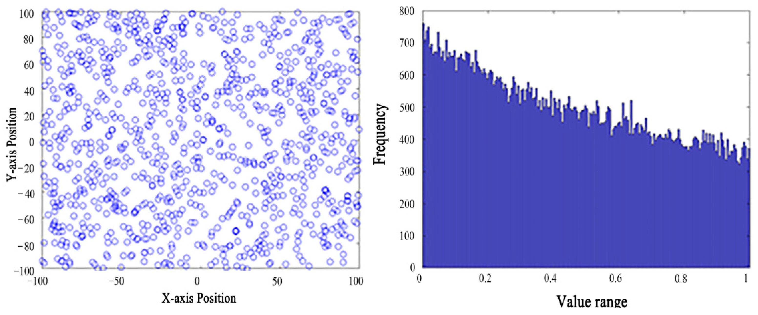
2.2.1. Population Initialization Based on Gauss Mapping

The phenomenon of chaos represents the presence of uncertainty and unpredictability within a deterministic system. Chaotic mappings have the ability to generate relatively uniformly distributed random numbers between 0 and 1. The initialization of the grey wolf population in the GWO algorithm has a certain impact on the stability and optimality of the overall algorithm. Different chaotic mappings yield different effects on the population initialization concerning population diversity and the extensive range of wolf search. Among them, the grey wolf population initialized using the Gauss chaotic mapping demonstrates a more uniform spatial distribution. Hence, this paper adopts the Gauss chaotic mapping for population initialization. The mathematical model is as follows:

$$x_{k+1}=\left\{\begin{array}{ll}0,\hfill & x_k=0\hfill \\ \frac{1}{x_{k}mod(1)},\hfill & otherwise \hfill \end{array}\right.$$

(8)

$$\frac{1}{x_{k}mod(1)}=\frac{1}{x_k}-\left[\frac{1}{x_k}\right]$$

(9)

Simulate the distribution of a population by randomly generating 1000 sample points over 1000 iterations. Describe the distribution of Gauss mapping values using a histogram. From Figure 3, it can be observed that the population initialized with Gauss mapping exhibits a relatively uniform spatial distribution and avoids the occurrence of local optima at the initial stages of the algorithm.

In cases where the population initialized with Gauss mapping continues to exhibit insufficient diversity, the utilization of reverse learning ensures population diversity by constructing reverse solutions based on the current population. The mathematical model for reverse learning is defined as follows:

$$\overline{X_{i,j}^e}=K\cdot \left({\alpha }_j+{\beta }_j\right)-X_{i,j}^e$$

(10)

In the equation, $X_{i,j}^e$ represents the j-th best solution corresponding to the i-th individual while $\overline{X_{i,j}^e}$ represents the corresponding reverse solution. ${\alpha }_j$ and ${\beta }_j$ are dynamic boundaries belonging to the minimum and maximum values in the best solution set, which helps prevent the reverse solutions from getting stuck in local optima. K is a dynamic coefficient ranging from 0 to 1. If certain reverse solutions exceed the dynamic boundaries, Gauss mapping is used for re-initialization.

Therefore, the introduction of the Gauss chaotic mapping helps to diversify the search space exploration. Chaotic maps exhibit sensitive dependence on initial conditions, which means that even small changes in the initial values can lead to significantly different trajectories. By employing Gauss chaotic mapping, the HI-GWO algorithm introduces a stochastic element that allows for better exploration of the solution space. This randomness enhances the algorithm’s ability to escape from local optima and find globally optimal solutions.

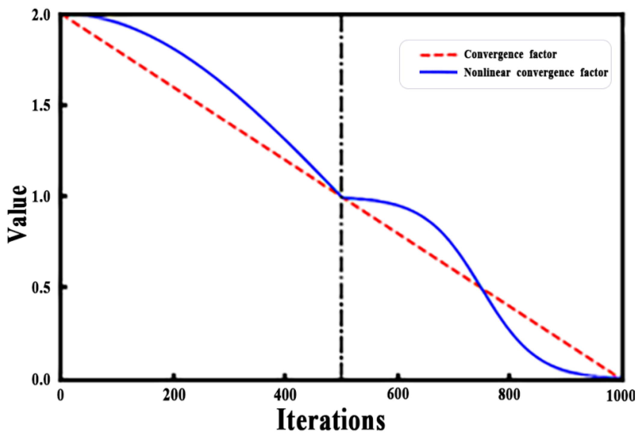
2.2.2. Nonlinear Convergence Factor

During the exploration phase, different individuals of grey wolves disperse and search for prey individually. In the exploitation phase, once prey is detected, all grey wolves come together. The GWO algorithm uses the coefficient vector $\overrightarrow{A}$ to simulate this behavior. When $\left|\overrightarrow{A}\right|$ > 1, the algorithm encourages grey wolves to separate from the currently found prey (local optima), thereby expanding the search range to find the global optimum. When $\left|\overrightarrow{A}\right|$ < 1, the algorithm reduces the search area, compelling the grey wolves to attack and hunt the prey.

According to Equation (3), the value of $\left|\overrightarrow{A}\right|$ is determined by the convergence factor a. In GWO, in order to reflect the grey wolves’ approach towards prey, a linearly decreases from 2 to 0. Correspondingly, the values of $\left|\overrightarrow{A}\right|$ also fluctuate within the range of [−a, a], indicating that the next position of a grey wolf may occur at any point between its current position and the prey. However, since the iterative process of the algorithm is nonlinear, using a linear convergence factor does not fully meet the requirements. Therefore, a nonlinear convergence factor adjustment strategy is introduced, expressed as follows:

$$\eta =\left\{\begin{array}{ll}1+\cos \frac{(t-1)\pi }{t_{\max }-1},\hfill & t\le \frac{t_{\max }}{2}\hfill \\ \frac{1}{1+\exp \left(\left(t-0.75t_{\max }\right)/\left(0.05t_{\max }\right)\right)},\hfill & t>\frac{t_{\max }}{2}\hfill \end{array}\right.$$

(11)

where t represents the current iteration count and t_max represents the maximum iteration count. Figure 4 compares the linear convergence factor with the improved nonlinear convergence factor.

The red dashed line represents the original linear convergence factor, while the blue solid line represents the improved nonlinear convergence factor. Based on the iteration curve, it can be concluded that the improved convergence factor divides the algorithm’s iterative process into two main parts, represented by the black dotted lines on both sides:

In the early stage of iteration, the convergence factor follows a cosine-like pattern, descending slowly in the first half. This ensures that the convergence factor remains mostly at larger values, thereby keeping the coefficient vector also at larger values. It expands the search range, improves global search capability, and avoids getting trapped in local optima.

In the later stage of iteration, there are two phases. In the first phase, considering the replacement of individuals within the population, the iteration curve shows a relatively gentle decline. At this point, the distance between the wolf pack and the prey increases, resulting in some energy loss.

In the second phase, the convergence factor quickly decreases and then stabilizes. This compensates for the time wasted in the previous phase. During this phase, the distance between the wolf pack and the prey starts to shorten. When the prey is surrounded, the convergence factor remains small for a long time, ensuring a focused search within a limited area. This enhances the algorithm’s local search capability and eventually initiates an attack on the prey.

In summary, the nonlinear convergence factor is an additional parameter introduced in the HI-GWO algorithm to control the convergence rate of the search process. The convergence factor adjusts the balance between exploration and exploitation during the optimization process. By incorporating nonlinearity into the convergence factor, the algorithm ensures that the search process gradually transitions from exploration to exploitation. Initially, the algorithm explores the solution space extensively to avoid premature convergence. As the optimization progresses, the algorithm gradually shifts its focus towards exploitation, refining the solutions found so far. This dynamic adjustment helps the algorithm strike a balance between global exploration and local exploitation, leading to improved performance.

2.2.3. Improve the Levy Flight Strategy

The Levy flight theory, employed in the GWO algorithm, is a random search strategy that allows for effective exploration of the solution space. It is inspired by Levy flights, which are random walks with long-distance steps that resemble the movement patterns found in certain animal populations. Levy flights are named after Paul Lévy, a French mathematician who first described them in the early 20th century. A Levy flight is a type of random walk where the step lengths follow a probability distribution called the Levy distribution. This distribution is characterized by heavy and long tails, meaning that it allows for occasional large step lengths that can span considerable distances, promoting global exploration in search spaces [24,25]. In the context of the GWO algorithm, the Levy flight theory is utilized to introduce randomness into the search process and enhance the algorithm’s ability to find global optima [26,27,28]. By incorporating the concept of Levy flights, the algorithm can make occasional long jumps during the search, which helps escape local optima and explore regions that may contain better solutions. Mathematically, the formula for the Levy flight theory can be expressed as:

$$s=\frac{\lambda •\mu }{{\left|v\right|}^{\frac{1}{\beta }}}$$

(12)

where s represents the obtained Levy flight step size, λ is a constant usually set to 1.5 as an empirical value, u is a random number sampled from a standard normal distribution, and v is a random number sampled from a Gamma distribution.

The Gamma function is used in Levy flight theory to generate random numbers that follow the Gamma distribution. The Gamma function is defined as follows:

$$\mathsf{\Gamma }\left(x\right)={\displaystyle {\int }_0^{\infty }{t}^{x-1}}{e}^{-t}dt$$

(13)

The Gamma function is an extension of the factorial function to the real numbers. For positive integers n, Γ (n) = (n − 1)! However, for non-integer and negative values of x, the value of the Gamma function can be obtained through integration.

In this article, a method is used to generate random numbers that follow the Levy distribution by using a normal distribution. The approach is as follows:

$$s=\frac{\mu }{{\left|v\right|}^{\frac{1}{\beta }}}$$

(14)

Here, $\mu \text{~}N\left(0,{\sigma }^2\right),v\text{~}N\left(0,1\right)$

$$\sigma ={\left\{\frac{\mathsf{\Gamma }\left(1+\beta \right)\sin \left(\frac{\pi \beta }{2}\right)}{\beta \mathsf{\Gamma }\left(\frac{1+\beta }{2}\right)2^{\frac{\beta -1}{2}}}\right\}}^{\frac{1}{\beta }}$$

(15)

To generate the next candidate solution $x_i^{\left(t+1\right)}$ at the current time $x_i^{\left(t\right)}$, use the formula mentioned below.

$$x_i^{\left(t+1\right)}=x_i^t+\theta \oplus levy\left(\beta \right)$$

(16)

where ⊗ denotes element-wise multiplication, $\theta$ is a random number between 0 and 1, and β is set to 1.5.

2.2.4. Golden Sine Algorithm

The improved golden sinusoidal operator in the GWO algorithm is a modified version of the original golden sinusoidal operator. The purpose of this modification is to enhance the diversity and convergence speed of the search process [29]. This section will provide a more detailed explanation of the concepts involved in the golden sinusoidal operator, as well as introduce the two adjusting parameters, r₁ and r₂, which control its scaling factor. The golden sinusoidal operator is inspired by the golden ratio, a mathematical constant denoted by the Greek letter phi, which is equal to approximately 1.6180339887. The golden ratio has remarkable properties that have captivated mathematicians for centuries due to its aesthetic appeal and prevalence in nature. It appears in various fields, including art, architecture, music, and even financial markets. In the context of optimization algorithms, the golden ratio can be integrated into an operator to improve the exploration-exploitation balance during the search process [30,31,32]. The operator utilizes sine functions to produce oscillations that guide the search towards promising regions in the solution space. The original golden sinusoidal operator does not consider any adjusting factors, leading to static oscillations throughout the entire optimization process. While it provides reasonable results, it may suffer from limited diversity and slower convergence rates. To address these limitations, the improved golden sinusoidal operator introduces two adjusting parameters, r₁ and r₂. The adjusting parameters, r₁ and r₂, control the scaling factor of the golden sinusoidal operator. By decreasing this scaling factor with an increasing number of iterations, the diversity of the search space is enhanced. This approach allows the GWO algorithm to explore a wider range of solutions at the beginning while focusing on local exploitation as the optimization progresses. The formula for the improved golden sinusoidal operator is as follows:

$$\left\{\begin{array}{c}b=1\\ r=\lambda \\ r_1=r\times 2\pi \\ r_2=r\times \pi \\ g=\frac{\sqrt{5}-1}{2}\\ X_1=\eta +(1-g)\times (b-\eta )\\ X_2=\eta +g\times (b-\eta )\end{array}\right.$$

(17)

Here, $\max t$ is the maximum number of iterations, $\lambda$ is a random number between 0 and 1, and g represents the golden ratio. By introducing the adjusting parameters r₁ and r₂, the improved golden sinusoidal operator dynamically adjusts the scaling factor during the search process, thereby enhancing the exploratory nature of the search space. This not only improves the algorithm’s global search capability but also accelerates the convergence speed.

2.2.5. Dynamic Position Update

In the GWO algorithm, the positions of the remaining individuals are updated based on the positions of the top three alpha, beta, and delta wolves in the grey wolf population. This update is influenced by the synchronous improvement of a nonlinear convergence factor. It aims to balance the global and local search capabilities of the algorithm. By combining the Levy flight strategy and the improved golden sinusoidal algorithm, the updated expression for position update is as follows:

$$X(t+1)=\left\{\begin{array}{cc}0.5\times (Levy\times X_{\alpha }-A\times D_{\alpha }+Levy\times X_{\beta })+Levy& if A<0.3\\ X\times \left|\sin (r_1)\right|-r_2\times \sin (r_1)\times \left|X_1\times D_{\alpha }-X_2\times X\right|& else\end{array}\right.$$

(18)

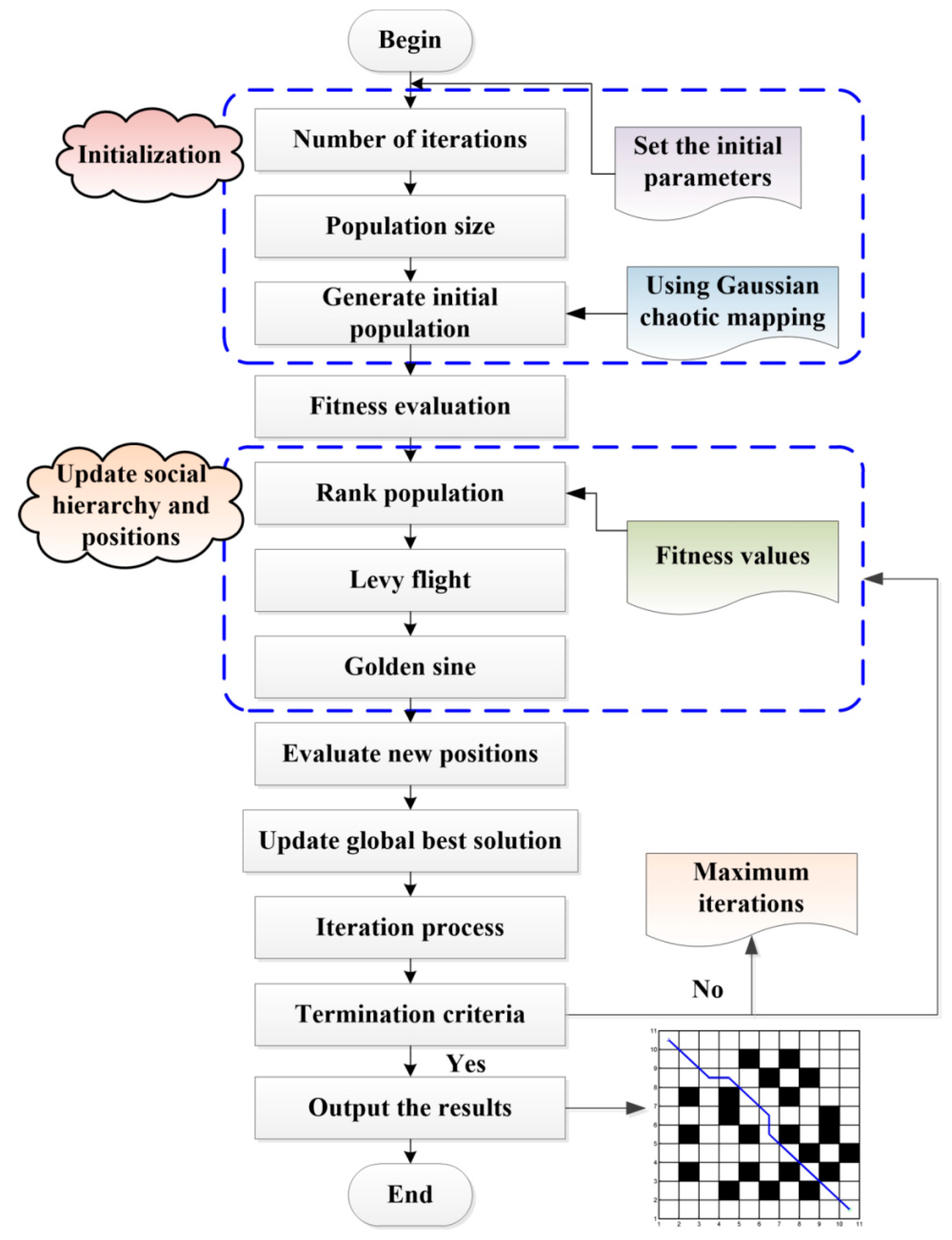
2.3. Implementation Steps of the Proposed Algorithm

This study proposes an enhanced HI-GWO algorithm to address the challenges faced by traditional swarm intelligence algorithms in mobile robot path planning. These challenges include low convergence accuracy, slow iteration speed, and susceptibility to local optima. The HI-GWO algorithm incorporates several key enhancements to overcome these limitations and improve performance. The specific implementation steps of the HI-GWO algorithm proposed in this article are as follows:

Step 1: 

Initialization. Set the number of iterations, population size, and other relevant parameters. Generate the initial population using Gaussian chaotic mapping to enhance population diversity.

Step 2: 

Fitness evaluation. Calculate the fitness value for each individual as a measure of the solution quality.

Step 3: 

Update social hierarchy and positions. Rank the population based on fitness values to establish the social hierarchy within the grey wolf pack. Higher-ranked wolves are more likely to become leaders, while lower-ranked ones play subordinate roles. Introduce Levy flight and sine algorithm to update the positions of each individual. Levy flight allows for longer jumps, exploring distant areas to enhance global search capability. The sine algorithm guides the search towards the most promising regions, improving solution accuracy and search speed.

Step 4: 

Evaluate new positions. Compute the fitness value for each individual at their updated positions.

Step 5: 

Update the global best solution. Update the global best solution based on the current best solution and its fitness value.

Step 6: 

Termination criteria. Check if the termination criteria, such as maximum iterations or fitness threshold, are met.

Step 7: 

Iteration process. If the termination criteria are not met, repeat steps 3 to 6. Continuously update individuals’ positions using the Levy flight and sine algorithm and calculate their fitness values.

Step 8: 

Output the result. Output the obtained final optimal solution as the solution for mobile robot path planning.

By following the above process, the HI-GWO algorithm utilizes Gaussian chaotic mapping in the initialization phase to generate diverse populations. When updating positions, the algorithm combines the Levy flight and sine algorithm along with a nonlinear convergence factor to balance global exploration and local exploitation capabilities. Levy flight enables long-distance jumps, exploring far-reaching areas, while the sine algorithm guides the search toward the most promising regions. Through continuous updates of social hierarchy, positions, and fitness values during the iteration process, the HI-GWO algorithm is capable of finding efficient solutions for mobile robot path planning. It demonstrates remarkable optimization ability, convergence accuracy, and robustness in various complex scenarios. Figure 5 represents the proposed algorithm flowchart.

The simulation experiments were conducted on a laptop running Windows 10 with an Intel i5 processor and 8GB of memory. The programming environment used was MATLAB 2017a. All algorithms were initialized with a population size of 30 and a maximum iteration count of 500 to ensure fairness in the experimental results. Other parameters were kept consistent across all experiments. Each program was independently executed 100 times, and the average value and standard deviation of the final computational results were taken as evaluation metrics.

3. Results and Discussion

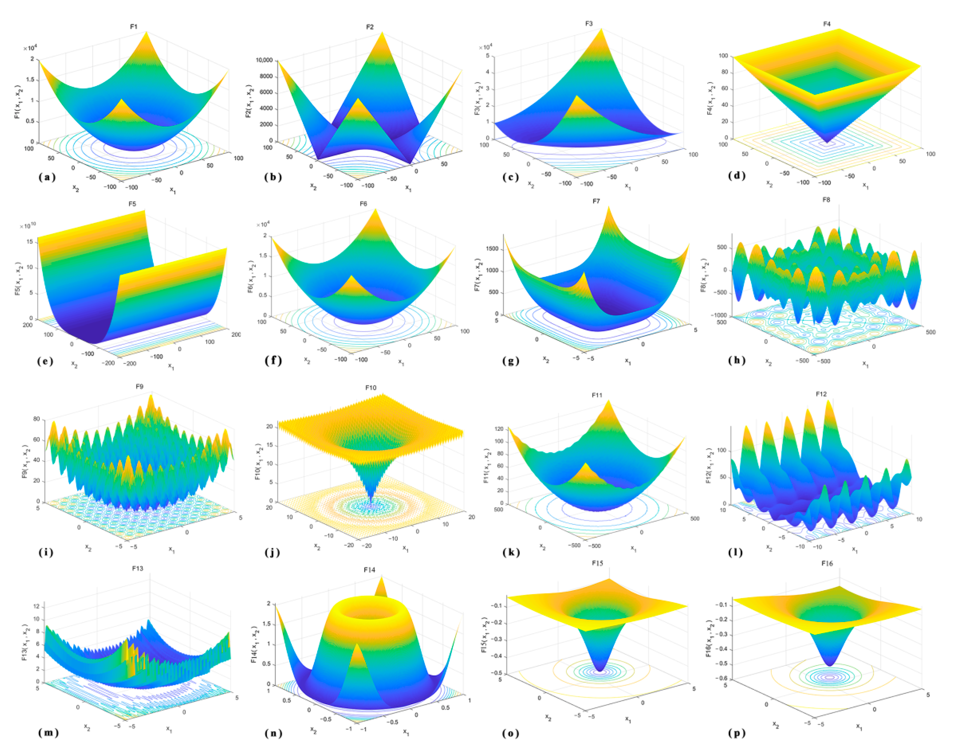
3.1. Standard Test Functions

In this study, 16 standard test functions commonly used internationally were selected to simulate and evaluate the HI-GWO algorithm. The basic information of these test functions is shown in

Table A1. Seven internationally recognized unimodal test functions.

Function Name	Function Expression	Domain	Dimension	Optimal Solution
f1	$f_1\left(x\right)={\displaystyle \sum _{i=1}{x}_i^2}$	[−100, 100]	30	0
f2	$f_2\left(x\right)={\displaystyle \sum _{i=1}^n\left|x_i\right|}+{\displaystyle \prod _{i=1}^n\left|x_i\right|}$	[−10, 10]	30	0
f3	$f_3\left(x\right)={{\displaystyle \sum _{i=1}^n\left({\displaystyle \sum _{j=1}^i{x}_j}\right)}}^2$	[−100, 100]	30	0
f4	$f_4\left(x\right)=Max\left\{\left|x_i\right|,1\le i\le D\right\}$	[−100, 100]	30	0
f5	$f_5\left(x\right)={\displaystyle \sum _{i=1}^{n-1}\left[100{\left(x_i+1-x_i^2\right)}^2+{\left(x_i-1\right)}^2\right]}$	[−30, 30]	30	0
f6	$f_6\left(x\right)={{\displaystyle \sum _{i=1}^n\left(x_i+0.5\right)}}^2$	[−100, 100]	30	0
f7	$f_7\left(x\right)={\displaystyle \sum _{i=1}^{n}i{x}_i^4}+random\left[0,1\right]$	[−128, 128]	30	0

,

Table A2. Six internationally recognized multimodal test functions.

Function Name	Function Expression	Domain	Dimension	Optimal Solution
f8	$f_8\left(x\right)={\displaystyle \sum _{i=1}^n-x_i}\sin \left(\sqrt{\left|x_i\right|}\right)$	[−500, 500]	30	−419.98 × Dim
f9	$f_9\left(x\right)={\displaystyle \sum _{i=1}^n\left[x_i^2-10\cos \left(2\pi x_i\right)+10\right]}$	[−5.12, 5.12]	30	0
f10	$\begin{array}{l}{f}_{10}\left(x\right)=20\exp \left(-0.2\frac{1}{n}{\displaystyle \sum _{i=1}^n{x}_i^2}\right)\\ -\exp \left(\frac{1}{n}{\displaystyle \sum _{i=1}^n\cos \left(2\pi x_i\right)}\right)+e+20\end{array}$	[−32, 32]	30	0
f11	$f_{11}\left(x\right)=\frac{1}{4000}{\displaystyle \sum _{i=1}^n{x}_i^2}-{\displaystyle \prod _{i=1}^n\cos \frac{x_i}{\sqrt{i}}}+1$	[−600, 600]	30	0
f12	$\begin{array}{l}{f}_{12}\left(x\right)= \frac{\pi }{n}\left({\displaystyle \sum _{i=1}^n{\left(y_i-1\right)}^2\left[1+10{\sin }^2\left(\pi y_{i+1}\right)\right]}\right)\\ +10\sin \left(\pi y_i\right)+{\left(y_n-1\right)}^2\\ +{\displaystyle \sum _{i=1}^{n}u\left(x_i,10,100,4\right)}\end{array}$	[−50, 50]	30	0
f13	$\begin{array}{l}{f}_{13}\left(x\right)=0.1{{\displaystyle \sum _{i=1}^{n-1}\left(x_i-1\right)}}^2\left[1+{\sin }^2\left(3\pi x_i+1\right)\right]\\ +{\sin }^2\left(3\pi x_i\right)+{\left(x_n-1\right)}^2\left[1+{\sin }^2\left(2\pi x_n\right)\right]\\ +{\displaystyle \sum _{i=1}^{n}u\left(x_i,5,100,4\right)}\end{array}$	[−50, 50]	30	0

and

Table A3. Three internationally recognized fixed-dimensional multimodal test functions.

Function Name	Function Expression	Domain	Dimension	Optimal Solution
f14	$f_{14}\left(x\right)=1-\cos \left(2\pi •\sqrt{{\displaystyle \sum x^2}}\right)$	[100, 100]	30	0
f15	$f_{15}\left(x\right)=-{{\displaystyle \sum _{i=1}^5\left[\left(x-a_i\right){\left(x-a_i\right)}^T+c_i\right]}}^{-1}$	[0, 10]	30	10.1532
f16	$f_{16}\left(x\right)=-{\displaystyle \sum _{i=1}^7\left[\left(x-a_i\right){\left(x-a_i\right)}^T+c_i\right]}$	[0, 10]	30	10.4028

. Among them, f₁ to f₇ are unimodal test functions that effectively demonstrate the convergence performance and solution accuracy of the algorithm. On the other hand, f₈ to f₁₀ are multimodal test functions used to measure the algorithm’s global search capability and ability to avoid local optima. Figure 6 showcases the plots of 16 standard benchmark functions, providing an overview of their characteristics and performance. The running parameters of each algorithm are shown in

Table 1. Running parameters of each algorithm.

Algorithms	PSO	WOA	DEA	DMOA	GWO	HI-GWO
Parameter configuration	c1 = 2; c2 = 2; Vmax = 2; Vmin = −2; ub = 100; lb = −100; Wmax = 0.8; Wmin = 0.2;	Pop = 50; Max_iter = 500	Pop = 50; Max_iter = 500; Crossover Rate = 0.8; Scaling Factor = 1.3	Pop = 50; Max_iter = 500; Mutation Rate = 0.2; Crossover Rate = 0.8	Pop = 50; Max_iter = 500	Pop = 50; Max_iter = 500

Note: In the provided code snippet, c₁ is used as the social cognitive parameter, representing the influence of the swarm’s collective knowledge on individual particles. Similarly, c₂ represents the self cognitive parameter, indicating the impact of an individual’s best position on their movement. V_max and V_min denote the maximum and minimum velocities, respectively, limiting the speed at which particles can explore the search space. Additionally, W_max and W_min represent the upper and lower bounds of the inertia weight, regulating the balance between exploration and exploitation during optimization. Pop refers to the population size, while Max_iter sets the maximum number of iterations for the algorithm to run.

.

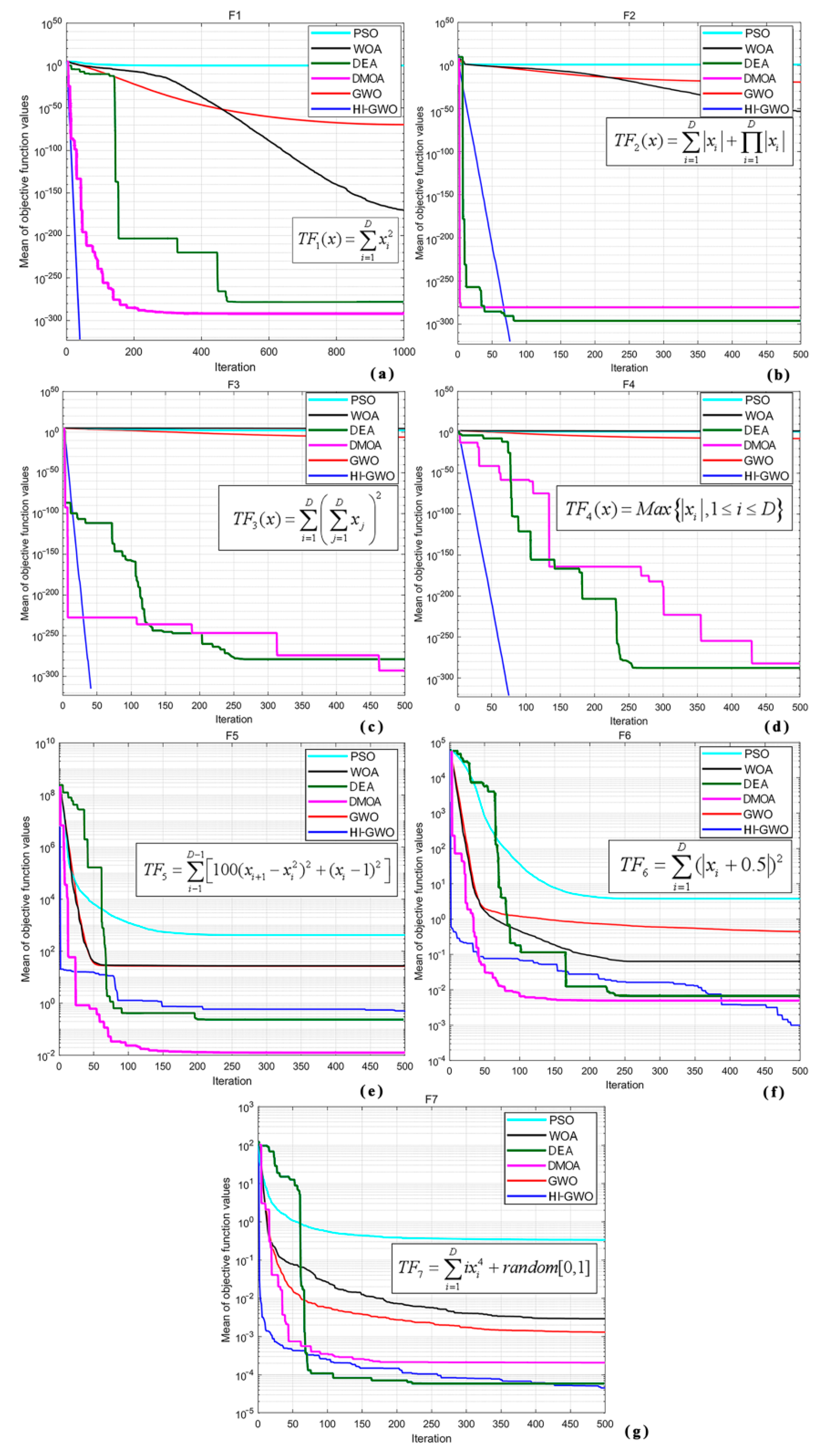
3.2. Analysis of Unimodal Test Function Experiments

Unimodal functions have only one global optimal solution. By using unimodal functions to test algorithms, we can evaluate their effectiveness in finding the global optimal solution. The simplicity and clear optimal solution of unimodal functions make the performance evaluation of algorithms more intuitive and reliable. Since unimodal functions have only one minimum value, they can be used to assess the performance of algorithm development, effectively demonstrating convergence performance and solution accuracy.

Table 2. Effectiveness verification results of HI-GWO Strategies (Dimension = 30).

Function Name	Metric	GWO	HI-GWO
f1	Worst value	1.44614 × 10−32	0
	Best value	0.000126387	0
	Mean value	2.28638 × 10−33	0
	Standard deviation	3.74166 × 10−33	0
f2	Worst value	2.21951 × 10−19	0
	Best value	1.46309 × 10−20	0
	Mean value	6.88322 × 10−20	0
	Standard deviation	5.2166 × 10−20	0
f3	Worst value	1.05028 × 10−6	0
	Best value	7.88338 × 10−11	0
	Mean value	7.88338 × 10−11	0
	Standard deviation	2.44756 × 10−7	0
f4	Worst value	7.95624 × 10−8	0
	Best value	2.80902 × 10−9	0
	Mean value	2.17452 × 10−8	0
	Standard deviation	2.07358 × 10−8	0
f5	Worst value	28.06617	1.1698
	Best value	25.65672333	0.000726383
	Mean value	26.726	0.1436413
	Standard deviation	0.682807333	0.316787233
f6	Worst value	0.316787233	0.012863687
	Best value	0.013620723	8.32301 × 10−6
	Mean value	0.447224667	0.001660262
	Standard deviation	0.302151333	0.003196104
f7	Worst value	0.00274467	0.00014252
	Best value	0.000345297	1.48734 × 10−6
	Mean value	0.001173079	4.05533 × 10−5
	Standard deviation	0.0006349	3.94767 × 10−5
f8	Worst value	−4153.945127	−12064.97969
	Best value	−7449.276533	−12569.34411
	Mean value	−6159.986437	−12472.28388
	Standard deviation	811.95658	139.31235
f9	Worst value	11.63951	0
	Best value	9.46667 × 10−15	0
	Mean value	1.967464	0
	Standard deviation	3.447013333	0
f10	Worst value	5.439 × 10−14	8.88 × 10−16
	Best value	3.62 × 10−14	8.88 × 10−16
	Mean value	4.321 × 10−14	8.88 × 10−16
	Standard deviation	4.62667 × 10−15	0
f11	Worst value	0.021814467	0
	Best value	0	0
	Mean value	0.00306005	0
	Standard deviation	0.0065315	0
f12	Worst value	0.079921333	0.001794702
	Best value	0.006867188	1.01184 × 10−6
	Mean value	0.028779633	0.000259836
	Standard deviation	0.017810267	0.00045103
f13	Worst value	0.835891667	0.00868251
	Best value	0.092272739	2.77073 × 10−6
	Mean value	0.403428667	0.001255902
	Standard deviation	0.192737333	0.00224423
f14	Worst value	0.21987	0
	Best value	0.099873	0
	Mean value	0.179786667	0
	Standard deviation	0.0411846	0
f15	Worst value	−4.223663333	−6.720826667
	Best value	−10.15290667	−10.15201333
	Mean value	−9.332596667	−9.44987
	Standard deviation	1.880446667	0.916336
f16	Worst value	−8.284113333	−7.15689
	Best value	−10.40266333	−10.40088667
	Mean value	−10.27821333	−9.079075862
	Standard deviation	0.503301063	0.912366

,

Table 3. Effectiveness verification results of HI-GWO Strategies (Dimension = 50).

Function Name	Metric	GWO	HI-GWO
f1	Worst value	1.82884 × 10−32	0
	Best value	2.34449 × 10−33	0
	Mean value	2.48493 × 10−33	0
	Standard deviation	4.68714 × 10−33	0
f2	Worst value	2.2836 × 10−19	0
	Best value	1.52938 × 10−20	0
	Mean value	6.9246 × 10−20	0
	Standard deviation	5.4266 × 10−20	0
f3	Worst value	1.5357 × 10−06	0
	Best value	1.077 × 10−10	0
	Mean value	1.14783 × 10−7	0
	Standard deviation	3.65209 × 10−7	0
f4	Worst value	8.21204 × 10−8	0
	Best value	2.88489 × 10−9	0
	Mean value	2.2739 × 10−8	0
	Standard deviation	2.13291 × 10−8	0
f5	Worst value	28.097954	1.2969124
	Best value	25.682092	0.000989726
	Mean value	26.733	0.14540434
	Standard deviation	0.6933128	0.33781164
f6	Worst value	1.1371116	0.01281442
	Best value	0.011864142	6.70086 × 10−6
	Mean value	0.4634684	0.001667801
	Standard deviation	0.3121814	0.003185422
f7	Worst value	0.002753862	0.000140153
	Best value	0.000342429	1.67117 × 10−6
	Mean value	0.001173874	0.000039824
	Standard deviation	0.000628745	3.8028 × 10−5
f8	Worst value	−4170.778866	−12054.79357
	Best value	−7448.306932	−12569.30542
	Mean value	−6156.813568	−12469.8668
	Standard deviation	808.394766	142.61796
f9	Worst value	10.857832	0
	Best value	6.816 × 10−15	0
	Mean value	1.7461292	0
	Standard deviation	3.1409356	0
f10	Worst value	5.401 × 10−14	8.88 × 10−16
	Best value	3.6294 × 10−14	8.88 × 10−16
	Mean value	4.3272 × 10−14	8.88 × 10−16
	Standard deviation	4.5862 × 10−15	0
f11	Worst value	0.022508466	0
	Best value	0	0
	Mean value	0.003030603	0
	Standard deviation	0.006597526	0
f12	Worst value	0.07430358	0.002090372
	Best value	0.006625902	1.08516 × 10−6
	Mean value	0.02885658	0.000277462
	Standard deviation	0.01676395	0.00051898
f13	Worst value	0.8048338	0.008343696
	Best value	0.082709289	2.27115 × 10−6
	Mean value	0.39817	0.001226874
	Standard deviation	0.1909844	0.002160486
f14	Worst value	0.21987	0
	Best value	0.099873	0
	Mean value	0.179945	0
	Standard deviation	0.04174324	0
f15	Worst value	−4.473606	−6.895714
	Best value	−10.15292	−10.150726
	Mean value	−9.392338	−9.459046939
	Standard deviation	1.809041703	0.8691754
f16	Worst value	−8.40935	−7.07988
	Best value	−9.986564	−10.400962
	Mean value	−10.280934	−9.362908163
	Standard deviation	0.478773796	0.9260868

and

Table 4. Effectiveness verification results of HI-GWO Strategies (Dimension = 100).

Function Name	Metric	GWO	HI-GWO
f1	Worst value	1.64031 × 10−32	0
	Best value	0.000037916	0
	Mean value	2.45833 × 10−33	0
	Standard deviation	4.18634 × 10−33	0
f2	Worst value	2.19035 × 10−19	0
	Best value	1.45757 × 10−20	0
	Mean value	6.7938 × 10−20	0
	Standard deviation	5.2027 × 10−20	0
f3	Worst value	0.028464289	0
	Best value	9.44162 × 10−11	0
	Mean value	5.74319 × 10−8	0
	Standard deviation	3.13539 × 10−7	0
f4	Worst value	9.04465 × 10−8	0
	Best value	2.8561 × 10−9	0
	Mean value	2.32812 × 10−8	0
	Standard deviation	2.28187 × 10−8	0
f5	Worst value	28.088809	1.1037777
	Best value	25.658486	0.000832102
	Mean value	26.733967	0.13026576
	Standard deviation	0.6925951	0.29332583
f6	Worst value	1.1169545	0.01252402
	Best value	0.006161516	5.10054 × 10−6
	Mean value	0.4524061	0.001622307
	Standard deviation	0.3092555	0.003107579
f7	Worst value	0.002753862	0.000140153
	Best value	0.000342429	1.67117 × 10−6
	Mean value	0.001173874	3.9824 × 10−5
	Standard deviation	0.000628745	3.8028 × 10−5
f8	Worst value	−4170.778866	−12054.79357
	Best value	−7448.306932	−12569.30542
	Mean value	−6156.813568	−12469.8668
	Standard deviation	808.394766	142.61796
f9	Worst value	10.857832	0
	Best value	7.384 × 10−15	0
	Mean value	1.7461292	0
	Standard deviation	3.1409356	0
f10	Worst value	5.40 × 10−14	8.88 × 10−16
	Best value	3.63 × 10−14	8.88 × 10−16
	Mean value	4.33 × 10−14	8.88 × 10−16
	Standard deviation	4.59 × 10−15	0.00
f11	Worst value	0.022508466	0
	Best value	0	0
	Mean value	0.003030603	0
	Standard deviation	0.006597526	0
f12	Worst value	0.07755977	0.00198497
	Best value	0.005989025	1.13393 × 10−6
	Mean value	0.02923882	0.000275676
	Standard deviation	0.017689595	0.000499535
f13	Worst value	0.7976553	0.011111255
	Best value	0.078658297	2.36804 × 10−6
	Mean value	0.3943197	0.001398812
	Standard deviation	0.1907708	0.002771557
f14	Worst value	0.21687	0
	Best value	0.099873	0
	Mean value	0.1790326	0
	Standard deviation	0.04212264	0
f15	Worst value	−4.564768	−6.920599
	Best value	−10.152923	−10.15062
	Mean value	−9.384764	−9.507023232
	Standard deviation	1.815354269	0.8893289
f16	Worst value	−8.5032	−6.816907
	Best value	−10.194624	−10.399588
	Mean value	−10.290876	−9.529245455
	Standard deviation	0.450210221	0.9985754

present the test result data for seven unimodal benchmark functions in dimensions of 30, 50, and 100 (f₁–f₇), with their function expressions shown in Table A1. Figure 7 also shows the convergence process curves of these seven unimodal functions under four different algorithms. The performance analysis of the HI-GWO algorithm was conducted on different dimensions of single-peaked functions (f₁ to f₄) in this study, revealing consistent superiority over the GWO algorithm in various aspects. Particularly, in the testing of function f₃, the HI-GWO algorithm achieved the theoretical optimum solution before just 50 iterations, while the convergence process of the GWO algorithm had only just begun. Furthermore, the HI-GWO algorithm exhibited superiority in terms of average worst value, best value, average value, and standard deviation, indicating its robustness. In contrast, even after 500 iterations, the GWO algorithm failed to reach the theoretical optimum solution, confirming the significantly faster convergence speed of HI-GWO over GWO. Comparisons were further made with other algorithms, such as Differential Evolutionary Algorithm (DEA), Dynamic Multi-Objective Optimization Algorithm (DMOA), Particle Swarm Optimization Algorithm (PSO), and Whale Optimization Algorithm (WOA) for handling single-peaked functions f₁ to f₄. The results demonstrated that the HI-GWO not only exhibited faster convergence but also had smaller fluctuations. For function f₂, in some cases, DEA and DMOA showed faster convergence but with lower robustness and accuracy. Overall, when the HI-GWO algorithm reached convergence, the convergence process of DEA, PSO, WOA, and other algorithms was just starting. Compared to GWO, DEA, PSO, WOA, and DMOA algorithms, the hybrid improved HI-GWO algorithm displayed higher convergence accuracy and stability, efficiently and stably finding the global optimum solution for single-peaked functions. For single-peaked functions f₅ to f₇, all algorithms successfully found the optimal solution, although slightly slower convergence was observed for HI-GWO in the testing of function f₂. However, it performed exceptionally well in the testing of other functions. In summary, HI-GWO demonstrated better capability in accurately identifying the optimal solution. Combining the analysis from Figure 6, the improved algorithm rapidly converged and found the optimal solution in the early iterations, significantly outperforming other algorithms in terms of speed. These results indicate that the improved algorithm surpasses GWO, WOA, PSO, DEA, and DMOA algorithms in terms of both convergence accuracy and speed.

By analyzing the experimental data of the aforementioned four algorithms under unimodal function conditions, it is evident that incorporating the improved Levy flight strategy and golden sine operator significantly enhances the algorithm’s computational power, improving convergence accuracy and speed and leading to outstanding performance in problem-solving scenarios.

3.3. Analysis of Multimodal Test Function Experiments

Multimodal functions have multiple local optima and one global optimum. By using multimodal functions to test algorithms, the performance of the algorithms in handling complex problems can be evaluated. Table 2, Table 3 and Table 4 present the test result data for six multimodal benchmark functions in different dimensions (f₈–f₁₃), with their function expressions shown in Table A2. Figure 6 also shows the convergence process curves of these six multimodal functions under four different algorithms. Analyzing the convergence curves of multimodal functions f₈–f₁₃ in Figure 8, it is evident that the HI-GWO algorithm outperforms the GWO algorithm in terms of convergence speed and accuracy, quickly finding the global optimal solution while GWO shows suboptimal performance. In the test of function f₈, DMOA and PSO did not start converging even after 450 iterations, indicating a slow convergence speed. DEA got trapped in local optima at 50 and 150 iterations, demonstrating a weaker ability to escape local optima. WOA and HI-GWO both achieved rapid and stable convergence, with HI-GWO outperforming WOA in terms of convergence speed. The GWO algorithm did not complete convergence even after 500 iterations, exhibiting fluctuating curves, poor robustness, and low accuracy. This highlights how the improved HI-GWO addresses the issue of traditional GWO algorithms tending to get trapped in local optima. In the test of function f₁₀, when reaching 100 iterations, the WOA algorithm got trapped in a local optimum, while DMOA and GWO achieved convergence but required more iterations. On the contrary, HI-GWO achieved convergence in only around ten iterations, demonstrating its remarkable speed. Overall, the results for functions f₈, f₉, f₁₀, and f₁₁ reveal a consistent pattern: PSO and GWO algorithms exhibit relatively slower convergence speeds in the initial stages, requiring more iteration to approach the optimal solution. In contrast, other algorithms achieve convergence and reach the theoretical optimum solution in the early stages. When comparing HI-GWO with DEA and DMOA, HI-GWO demonstrates faster convergence speed, while DEA and DMOA show slower convergence speed. The convergence speeds of PSO, WOA, and GWO are comparable but still slower than HI-GWO. Particularly, HI-GWO performs exceptionally well in handling functions f₁₂ and f₁₃.

It can be concluded that in the tests of multimodal functions, the HI-GWO algorithm exhibits faster optimization speed and higher accuracy in most cases. It also showcases superior global search and local optimization capabilities compared to traditional GWO algorithms, effectively overcoming the issue of getting trapped in local optima. Additionally, HI-GWO shows strong adaptability and robustness in handling complex multi-dimensional functions. Furthermore, the improved HI-GWO algorithm demonstrates greater robustness in multimodal testing of functions compared to PSO, WOA, DEA, DMOA, and GWO algorithms, highlighting the significant improvement in stability achieved by enhancing the nonlinear convergence factor.

Analyzing the performance of the four algorithms on multimodal functions, we find that the HI-GWO algorithm successfully balances global exploration and local exploitation through flexible search strategies, leading to better solutions in complex multimodal functions. The algorithm exhibits good convergence and can stably converge to the optimal solutions of different peaks in multimodal functions. Furthermore, the hybrid HI-GWO algorithm effectively escapes local optima and finds global optima, avoiding the problem of getting trapped in suboptimal solutions. It has been proven that the HI-GWO algorithm has a higher success rate, faster convergence speed, better adaptability, and robustness in optimization, enabling it to effectively handle complex problems.

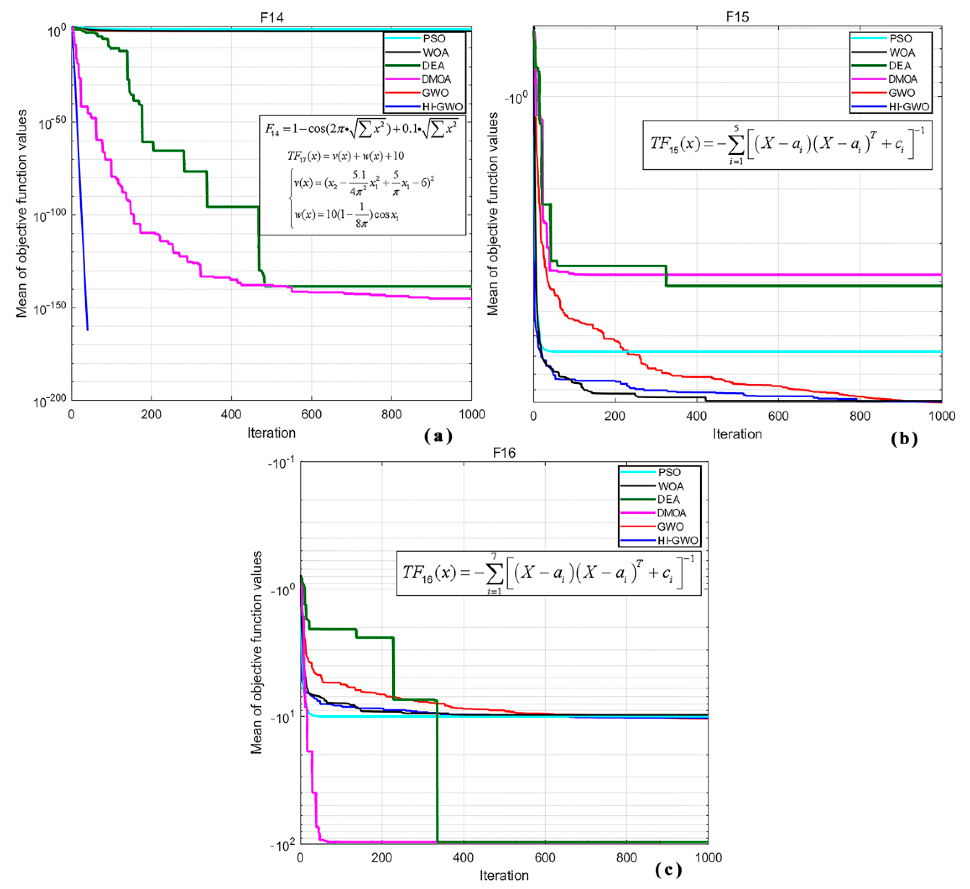
3.4. Analysis of Fixed-Dimensional Multimodal Test Function Experiments

Fixed-dimensional multimodal functions are a special case of multimodal functions where the number and positions of peaks remain constant throughout the entire search process. By using fixed-dimensional multimodal functions to test algorithms, we can more accurately evaluate their performance in handling problems with stable multimodal structures. This helps analyze the algorithm’s exploration strategies and convergence behavior in the search space. Table 2, Table 3 and Table 4 present the test result data for three fixed-dimensional multimodal benchmark functions in different dimensions (f₁₄–f₁₆), with their function expressions shown in Table A3. Figure 9 also shows the convergence process curves of these three fixed-dimensional multimodal functions under four different algorithms. In the test of function f₁₄, the HI-GWO algorithm achieved convergence and found the theoretical optimum value within 50 iterations, demonstrating faster speed compared to traditional GWO. DMOA and DEA also achieved convergence, but their speed was slower due to being influenced by local optima, with DEA exhibiting poorer robustness compared to DMOA. PSO and WOA were still in the initial stages of convergence. In the convergence curve of f₁₅, all six algorithms achieved convergence, with HI-GWO and WOA showing fast convergence speeds and similar curves, while the differences among the algorithms were not significant. Analyzing the convergence curve of f₁₆ revealed that all four algorithms found the optimal value, but HI-GWO exhibited a faster convergence speed than the other three algorithms, and DEA was trapped in local optima in the early stages.

By employing precise and efficient search strategies, the HI-GWO algorithm outperformed PSO, WOA, DEA, DMOA, and GWO algorithms in fixed-dimensional multimodal function testing, effectively narrowing down the search space and finding global optimum solutions. In most test cases, HI-GWO demonstrated superior convergence speed and accuracy compared to other algorithms. The HI-GWO algorithm also achieved excellent mean values and standard deviations across different dimensional tests.

In summary, analyzing the performance of the four algorithms on multimodal functions, it is found that the HI-GWO algorithm still demonstrates good adaptability and robustness, reliably finding the global optimum and avoiding getting trapped in local optima. The algorithm excels in solving fixed-dimensional multimodal testing function problems, demonstrating its ability to quickly and accurately locate the global optimum. It showcases strong potential for providing effective solutions to high-dimensional optimization problems and real-world scenarios, possessing a certain level of global exploration and local exploitation capabilities.

3.5. Experimental Analysis

Based on the experimental results comparing HI-GWO and GWO algorithms with different functions in various dimensions, as well as the convergence curves comparing HI-GWO, GWO, DEA, and DOMA algorithms for different functions, it is demonstrated that the HI-GWO algorithm outperforms the traditional GWO algorithm in terms of optimization capability, convergence speed, convergence accuracy, robustness, and adaptability.

The experimental data confirms the success of algorithmic improvements. The improvement of the convergence factor from linear to nonlinear in the GWO algorithm avoids premature convergence in the early iterations and enhances convergence speed in the later iterations. This balance between global and local search capabilities makes the algorithm more suitable for real-world scenarios. The improvement of the Levy flight strategy enhances global search capability and prevents getting trapped in local optima. The improvement of the golden sine operator significantly enhances diversity in the search process, convergence speed, and global search ability.

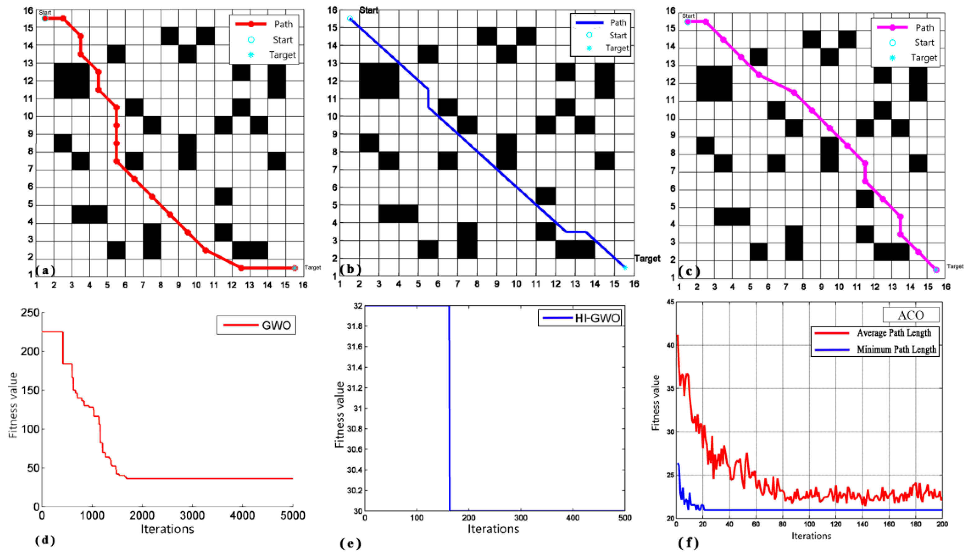
3.6. Mobile Robot Path Planning Simulation

Further research was conducted to investigate the optimization performance of the algorithm to verify the effectiveness of the HI-GWO algorithm in mobile robot path planning. Grid-based maps of different complexities were constructed using different obstacle rates, including 10 × 10, 15 × 15, 40 × 40, and 50 × 50 grids. In these maps, black grids represent obstacles in the environment, while white grids represent the movable area for the mobile robot. The robot, represented as a point, was constrained to navigate through empty cells while avoiding obstacles. It was equipped with perception capabilities to detect and understand obstacles and target points on the grid map. The results were evaluated by assessing the completeness of the generated path reaching the target, calculating the length of the path for efficiency analysis, verifying collision avoidance with obstacles, and measuring the number of turns and iterations in the generated path. The number of turns quantified the level of complexity in the path planning process, while the number of iterations reflected the iterative optimization of the algorithm.

ACO (Ant Colony Optimization) is a stochastic optimization algorithm inspired by the foraging behavior of ants. It simulates how ants communicate through pheromones to find the shortest path from their nest to a food source. Ants release pheromones on the paths they traverse, attracting other ants to follow those paths. They also reinforce the pheromone levels on successful paths [33,34]. ACO algorithm represents problem solutions as ants and optimization objectives as food sources. By adjusting the concentration of pheromones on paths, ACO optimizes the solution space. This algorithm has wide applications in combinatorial optimization, path planning, scheduling problems, and more, providing efficient global search capabilities and being easy to implement. Its heuristic nature makes ACO an important intelligent optimization algorithm.

The standard GWO, ACO and the HI-GWO algorithm were compared by running them independently, with the same initial parameters as in the previous function simulation: population size and maximum iteration count. The starting and ending points of the robot’s path were located in the top-left corner and bottom-right corner of the map, respectively. The algorithms were run 50 times independently, and the average values were taken as the final results. The path trajectories and convergence plots are shown in Figure 10 and Figure 11, while the metric test results are presented in

Table 5. Path Planning Test Results.

Algorithms	10 × 10			15 × 15
	Optimal Solution	Average Solution	Path Nodes	Optimal Solution	Average Solution	Path Nodes
ACO	20	31	[1,2,3,3,3,4,5,6,7,8]	28	32	[2,3,4,5,7,8,9,10,11,11,12,13,13,14]
GWO	22	34	[1,1,1,1,2,4,5,6,7,8]	32	36	[2,3,3,4,4,5,5,5,5,6,7,8,9,10,12]
HI-GWO	13	21.5	[1,2,3,4,5,6,6,7,8,9]	20	27	[1,2,3,4,5,5,6,7,8,9,10,11,12,13,14]

.

The above experiments demonstrate that both the GWO and HI-GWO algorithms can be successfully applied to path planning, as they can search for feasible paths in different maps. Based on the optimal path length and average values shown in the table, it can be concluded that the standard GWO algorithm has poor stability. The path generated by the standard GWO algorithm contains many turning points, lacks smoothness, and exhibits insufficient local exploration capability during the later iterations, leading to the algorithm getting trapped in local optima. In contrast, this paper improves the HI-GWO algorithm by integrating both global and local search capabilities. In the initial stage of the algorithm, through population initialization and reverse learning, the global exploratory ability is enhanced, resulting in high-quality and diverse initial solutions while avoiding being trapped in local optima. Additionally, the introduction of a nonlinear convergence factor and dynamic position updates strengthens the local search capability in the later stages of the algorithm, ensuring result stability. The HI-GWO algorithm generates path lengths shorter than those of the standard GWO, and the resulting paths are relatively smooth, yielding excellent results.

The experiment constructed 2D grid simulation maps with sizes of 40 × 40 and 50 × 50 to simulate real-world path planning scenarios. Path planning experiments were conducted in environments with obstacle rates of 10%, 15%, and 20%. The generated planning paths (lines) from each algorithm are shown in the figures. Additionally, using a grid cell side length as one unit, the path lengths and number of turns for each path were calculated based on the acquired data. These results were organized into a comparative table (

Table 6. Comparing algorithm metrics across different scenarios.

Algorithm	Map Dimension	Obstacle Rate	Path Length	Iteration	Number of Turns
ACO	40 × 40	10%	69.1543	200	35
GWO			67.3917	170	25
HI-GWO			57.4222	160	17
ACO		15%	75.3969	220	35
GWO			70.0652	180	23
HI-GWO			57.8782	160	11
ACO		20%	70.0833	300	46
GWO			101.4727	290	25
HI-GWO			60.1767	210	19
ACO	50 × 50	10%	124.0243	400	80
GWO			96.3207	350	29
HI-GWO			71.5382	300	11
ACO		15%	95.0538	410	77
GWO			92.9756	370	34
HI-GWO			77.0133	320	15
ACO		20%	102.468	490	101
GWO			86.6332	450	34
HI-GWO			77.7915	380	24

) presenting various metrics for different algorithms under different scenarios. This study aims to provide insights into path planning techniques applicable to real-world situations.

Based on the presented simulation results in Figure A1, it can be clearly observed that under different obstacle density conditions, the path obtained by the ACO algorithm exhibits significant deficiencies. The characteristics of this path include fewer straight segments but a significantly longer length compared to the paths generated by the HI-GWO and GWO algorithms. In contrast, the GWO algorithm shows overall longer and more convoluted route planning, failing to achieve the desired outcome. However, the HI-GWO algorithm demonstrates outstanding performance with the smoothest and shortest path length, allowing for faster arrival at the destination. Compared to the other two methods, the HI-GWO algorithm exhibits higher globality in path selection, providing more favorable conditions for finding the optimal path. By analyzing the comparative data of various indicators for different algorithms in different scenarios, it can be observed that in all experimental groups, the HI-GWO algorithm consistently yields the lowest path length and also has the fewest number of turns.

Table 7. HI-GWO Overperformance Ratio.

Algorithm	Map Dimension	Obstacle Rate	Path Length Ratio	Number of Iteration Ratio	Number of Turns Ratio
ACO	40 × 40	10%	16.97%	20.00%	51.43%
GWO			14.17%	5.88%	32.00%
ACO		15%	23.24%	18.18%	68.57%
GWO			17.39%	11.11%	52.17%
ACO		20%	14.14%	30.00%	58.69%
GWO			40.69%	27.58%	24.00%
ACO	50 × 50	10%	42.32%	25.00%	86.24%
GWO			25.735	14.29%	62.06%
ACO		15%	18.89%	21.95%	80.52%
GWO			17.17%	13.51%	55.88%
ACO		20%	24.08%	22.44%	76.23%
GWO			10.20%	15.56%	29.41%

demonstrates that the proposed HI-GWO algorithm maintains a significant advantage over path length, iteration, and number of turns.

In the experiments conducted on a 40 × 40 and 50 × 50 grid map (Figure A1), the HI-GWO algorithm exhibited significant improvements over the GWO algorithm. On average, the HI-GWO algorithm reduced the path length by 18.84 units and decreased the number of turns by 12 compared to the GWO algorithm. Furthermore, compared to the ACO algorithm, the HI-GWO algorithm achieved an average reduction in path length by 32.04 units and decreased the number of turns by 46. The data also indicate that as the size of the map increases, and the obstacle density rises, the disparity between the GWO and ACO algorithms versus the HI-GWO algorithm becomes more pronounced. This reflects the ability of the HI-GWO algorithm to compute optimal paths even for more complex problems, demonstrating its strong globality and robustness.

For instance, in the experiment conducted on a 50 × 50 grid map with a 20% obstacle density (Figure A1), the HI-GWO algorithm achieved the shortest path length among the three algorithms, measuring 77.7915 units. It had only 24 turns, and the path closely resembled a straight line connecting the start and end points. In contrast, the GWO algorithm’s path exhibited more bends with 34 turns. Many segments of its path were trapped in local optima within specific regions of the map, leading to a significantly increased path length. The ACO algorithm’s path was even more convoluted, measuring 102.468 units, and it performed relatively worse compared to the HI-GWO Algorithm. It had 101 turns, which was the highest among the three algorithms. Through calculations, it was discovered that in the experiment conducted on a 50 × 50 grid map with a 20% obstacle density, the HI-GWO algorithm achieved a 10.20% reduction in path length and a 29.41% decrease in the number of turns compared to the HI-GWO algorithm. Furthermore, compared to the ACO algorithm, the HI-GWO algorithm achieved a 24.08% reduction in path length and a 76.23% decrease in the number of turns. To present the superiority of HI-GWO more explicitly, Figure A2 illustrates the performance comparison values among different algorithms. These results demonstrate the superiority of the HI-GWO algorithm over other algorithms, highlighting the significant improvement in optimization capability achieved through the incorporation of the Levy flight strategy and the golden sine operator. These enhancements greatly enhance the efficiency of the algorithm. The patterns and characteristics exhibited by the three algorithms in this experiment have also been validated in other experimental groups.

The research findings indicate that compared to traditional GWO and ACO algorithms, their search efficiency is low, and convergence speed is slow, making them prone to local optima. However, when compared to these two traditional algorithms, the HI-GWO algorithm demonstrates excellent global convergence ability and achieves optimal convergence. It effectively shortens the path length and reduces the runtime. Additionally, the algorithm exhibits high stability in overall operation without significant occurrences of large local bends. This indicates that the HI-GWO algorithm has a higher success rate in the optimization process than the other three methods and demonstrates a strong ability to escape local optima. The comparative experimental results lead to the conclusion that in path planning tasks, the HI-GWO algorithm, as an improved version, can generate shorter and smoother routes compared to the original algorithm and other comparative methods.

The findings from simulations and experiments provide valuable insights into the real-world applicability of the proposed HI-GWO algorithm. This algorithm holds potential benefits for various scenarios and industries that involve mobile robot path planning. One area where the algorithm could be beneficial is autonomous transportation, such as self-driving cars or delivery robots. The HI-GWO algorithm’s ability to optimize paths can help these vehicles navigate efficiently and safely through complex road networks, minimizing travel time and reducing congestion. Another application lies in industrial automation, where mobile robots are utilized for tasks like warehouse management or manufacturing processes. By using the HI-GWO algorithm, these robots can determine optimized paths to navigate through dynamic environments efficiently, maximizing productivity and minimizing resource utilization. Furthermore, the algorithm can find its applications in search and rescue missions. During emergency situations or natural disasters, mobile robots equipped with the HI-GWO algorithm can quickly generate optimal paths to explore and locate survivors, improving search efficiency and potentially saving lives. Additionally, the algorithm’s ability to strike a balance between global exploration and local exploitation can be beneficial in environmental monitoring and surveillance. Mobile robots equipped with sensors can utilize the HI-GWO algorithm to plan paths that cover a wide area while focusing on critical regions for data collection, enabling effective monitoring of ecological systems or security surveillance.

However, The HI-GWO algorithm introduces several trade-offs that should be considered in the discussion. One potential trade-off is the balance between increased global search capability and longer computation times. The increased global search capability of the HI-GWO algorithm allows for a more comprehensive exploration of the solution space, potentially leading to better optimization performance. By incorporating hierarchical structures and multiple levels of groups and individuals, the algorithm can explore diverse regions and avoid getting trapped in local optima. However, this increased global search capability may come at the cost of longer computation times. The additional iterations and evaluations required by the algorithm to explore the solution space can lead to increased computational overhead. Depending on the complexity of the problem and the specific implementation of the algorithm, the time required to converge to an optimal solution may be longer compared to other optimization algorithms. It is important to note that the trade-off between global search capability and computation time may vary depending on the problem being solved and the specific requirements of the application. In some cases, the improved exploration provided by the HI-GWO algorithm may compensate for the longer computation times, resulting in better overall optimization performance. To mitigate the potential trade-off, researchers can explore strategies to optimize the efficiency of the HI-GWO algorithm. This can include fine-tuning parameters, implementing parallel computing techniques, or utilizing hardware acceleration to reduce computation times while maintaining the benefits of enhanced global search capabilities. Addressing these trade-offs adds nuance to the discussion by recognizing that the choice between increased global search capability and computation time depends on the specific problem and context. Balancing these factors ensures that the HI-GWO algorithm is effectively applied in practical scenarios, taking into account the desired trade-offs for optimal performance.

The proposed enhanced HI-GWO addresses challenges in traditional swarm intelligence algorithms for mobile robot path planning. However, there are several limitations and challenges that need to be considered. One challenge is the computational complexity of the algorithm, as path planning problems are typically NP-hard. This may result in longer execution times, especially for large-scale maps, requiring further optimization for practical efficiency. The algorithm is also sensitive to parameter selection, which can affect the quality of the paths generated or even lead to failure in reaching the target point. Careful parameter tuning is necessary to achieve desirable results. Additionally, the algorithm’s robustness is a limitation. It may exhibit poorer performance when faced with complex environmental changes or uncertainties. Further improvements and adaptive designs may be needed for real-world scenarios. Furthermore, finding the optimal trade-off between exploration and exploitation is challenging. Different problem domains may require different degrees of emphasis on these aspects, affecting the algorithm’s performance. Addressing these challenges and limitations is important for the effective application of the proposed HI-GWO algorithm in practical scenarios. Further research is needed to refine the algorithm, optimize parameter settings, and evaluate its performance in various real-world applications.

4. Conclusions

In conclusion, the HI-GWO algorithm proposed in this study offers practical implications that contribute to the advancement of mobile robot path planning. By addressing the limitations of traditional swarm intelligence algorithms, the HI-GWO algorithm improves convergence accuracy, iteration speed, and robustness in diverse and complex scenarios. The key enhancements incorporated into the algorithm, including Gauss chaotic mapping for population initialization and the novel nonlinear convergence factor, enable effective exploration of the solution space while refining the search in promising regions. The adaptive position update strategy combining Levy flight and golden sine further enhances solution accuracy, global search capability, and search speed. Extensive simulations on benchmark functions demonstrate the effectiveness of the HI-GWO algorithm, outperforming other state-of-the-art intelligent algorithms in terms of optimization performance. Moreover, a real-world path planning experiment confirms its superior efficiency over traditional grey wolf and ant colony algorithms.

The HI-GWO algorithm’s practical contributions lie in its ability to provide a more effective and efficient optimization approach for mobile robot path planning. Its improvements in convergence accuracy, iteration speed, and robustness make it suitable for various practical applications. These include optimizing travel time and energy consumption in warehouse automation, autonomous transportation, and search and rescue missions. Additionally, the algorithm’s capacity to handle complex environments and adapt to different mobile robot platforms expands its applicability and increases operational safety.

References

1. Yahia, H.S.; Mohammed, A.S. Path planning in Unmanned Aerial Vehicles (UAVs): Overview, Challenges, and Solutions. Util. Math. 2023, 120, 455–471. [Google Scholar]
2. Liu, L.; Wang, X.; Yang, X.; Liu, H.; Li, J.; Wang, P. Path planning techniques for mobile robots: Review and prospect. Expert Syst. Appl. 2023, 227, 120254. [Google Scholar] [CrossRef]
3. Sabitri, P.; Muhammad, Y.; Sangman, M. Bio-Inspired Optimization-Based Path Planning Algorithms in Unmanned Aerial Vehicles: A Survey. Sensors 2023, 23, 3051. [Google Scholar]
4. Faten, A.; Heba, K.; Kamal, Y. Bio-Inspired Multi-UAV Path Planning Heuristics: A Review. Mathematics 2023, 11, 2356. [Google Scholar]
5. Jaafar, A.; Dheyaa, J. Lassical and Heuristic Approaches for Mobile Robot Path Planning: A Survey. Robotics 2023, 12, 93. [Google Scholar]
6. Hazha, S.; Amin, S. Path planning optimization in unmanned aerial vehicles using meta-heuristic algorithms: A systematic review. Environ. Monit. Assess. 2023, 195, 30. [Google Scholar]
7. Selcuk, A.; Tevfik, E. An immune plasma algorithm based approach for UCAV path planning. J. King Saud Univ. Comput. Inf. Sci. 2023, 35, 56–69. [Google Scholar]
8. Ma, Z.; Chen, J. Adaptive path planning method for UAVs in complex environments. Int. J. Appl. Earth Obs. Geoinf. 2022, 115, 103133. [Google Scholar] [CrossRef]
9. Vincent, R.; Tarbouchi, M. Hybrid deterministic non-deterministic data-parallel algorithm for real-time unmanned aerial vehicle trajectory planning in CUDA. e-Prime-Adv. Electr. Eng. Electron. Energy 2022, 2, 100085. [Google Scholar]
10. Wei, Y.; Feng, J.; Huang, Y.; Liu, K.; Ren, B. Path Planning of Mobile Robot Based on Improved Genetic Algorithm. J. Supercomput. 2022, 2365, 012053. [Google Scholar] [CrossRef]
11. Yao, P.; Zhao, S. Three-Dimensional Path Planning for AUV Based on Interfered Fluid Dynamical System Under Ocean Current (June 2018). Inst. Electr. Electron. Eng. 2018, 6, 42904–42916. [Google Scholar] [CrossRef]
12. Chen, Q.; He, Q.; Zhang, D. UAV Path Planning Based on an Improved Chimp Optimization Algorithm. Axioms 2023, 12, 702. [Google Scholar] [CrossRef]
13. Wang, X.; Pan, J.; Yang, Q.; Kong, L.; Snášel, V.; Chu, S. Modified Mayfly Algorithm for UAV Path Planning. Drones 2022, 6, 134. [Google Scholar] [CrossRef]
14. Manikandan, K.; Sriramulu, R. Optimized Path Planning Strategy to Enhance Security under Swarm of Unmanned Aerial Vehicles. Drones 2022, 6, 336. [Google Scholar] [CrossRef]
15. Jarray, R.; Bouallègue, S.; Rezk, H.; Al-Dhaifallah, M. Parallel Multiobjective Multiverse Optimizer for Path Planning of Unmanned Aerial Vehicles in a Dynamic Environment with Moving Obstacles. Drones 2022, 6, 385. [Google Scholar] [CrossRef]
16. Zheng, L.; Tian, Y.; Wang, H.; Hong, C.; Li, B. Path Planning of Autonomous Mobile Robots Based on an Improved Slime Mould Algorithm. Drones 2023, 7, 257. [Google Scholar] [CrossRef]
17. Panwar, K.; Dee, K. Discrete Grey Wolf Optimizer for symmetric travelling salesman Problemp. Appl. Soft Comput. 2021, 105, 107298. [Google Scholar] [CrossRef]
18. Muni, M.; Parhi, D.; Priyadarshi, K. Implementation of grey wolf optimization controller for multiple humanoid navigation. Comput. Animat. Virtual Worlds 2020, 31, e1919. [Google Scholar] [CrossRef]
19. Sun, L.; Feng, B.; Chen, T.; Zhao, D.; Xin, Y. Equalized GreyWolfOptimizer with Refraction Opposite Learning. Comput. Intell. Neurosci. 2022, 2022, 2721490. [Google Scholar] [CrossRef]
20. Li, J.; Yang, F. Task assignment strategy for multi-robot based on improved Grey Wolf Optimizer. J. Ambient Intell. Humaniz. Comput. 2020, 12, 6319–6335. [Google Scholar] [CrossRef]
21. Xu, C.; Xu, M.; Yin, C. Optimized multi-UAV cooperative path planning under the complex confrontation environment. Comput. Commun. 2020, 162, 196–203. [Google Scholar] [CrossRef]
22. Qu, C.; Gai, W.; Zhang, J.; Zhong, M. A novel hybrid grey wolf optimizer algorithm for unmanned aerial vehicle (UAV) path planning. Knowl. Based Syst. 2020, 194, 105530. [Google Scholar] [CrossRef]
23. Liu, J.; Wei, X.; Huang, H. An Improved Grey Wolf Optimization Algorithm and Its Applicationin Path Planning. Inst. Electr. Electron. Eng. 2021, 9, 121944–121956. [Google Scholar]
24. Mesa, A.; Castromayor, K.; Garillos-Manliguez, C.; Calag, V. Cuckoo search via Levy flights applied to uncapacitated facility location problem. J. Ind. Eng. Int. 2017, 14, 585–592. [Google Scholar] [CrossRef]
25. Wang, Y.; Yu, X.; Yang, L.; Li, J.; Zhang, J.; Liu, Y.; Sun, Y.; Yan, F. Research on Load Optimal Dispatch for High-Temperature CHP Plants through Grey Wolf Optimization Algorithm with the Levy Flight. Processes 2022, 10, 1546. [Google Scholar] [CrossRef]
26. Chen, Z.; Yu, Y.; Wang, Y. Parameter Identification of Jiles-Atherton Model Based on Levy Whale Optimization Algorithm. IEEE Access 2022, 10, 66711–66721. [Google Scholar] [CrossRef]
27. Gupta, S.; Deep, K. Enhanced leadership-inspired grey wolf optimizer for global optimization problems. Eng. Comput. 2019, 36, 1777–1800. [Google Scholar] [CrossRef]
28. Karakoyun, M.; Ozkis, A.; Kodaz, H. A new algorithm based on gray wolf optimizer and shuffled frog leaping algorithm to solve the multi-objective optimization problems. Appl. Soft Comput. J. 2020, 96, 106560. [Google Scholar] [CrossRef]
29. Li, Z. A local opposition-learning golden-sine grey wolf optimization algorithm for feature selection in data classification. Appl. Soft Comput. 2023, 142, 110319. [Google Scholar] [CrossRef]
30. Tanyildizi, E.; Demir, G. Golden Sine Algorithm: A Novel Math-Inspired Algorithm. Adv. Electr. Comput. Eng. 2017, 17, 71–78. [Google Scholar] [CrossRef]
31. Tanyildizi, E. A novel optimization method for solving constrained and unconstrained problems: Modified Golden Sine Algorithm. Turk. J. Electr. Eng. Comput. Sci. 2018, 26, 3287–3304. [Google Scholar] [CrossRef]
32. Yang, X.; Cheng, L. Hyper-spectral Image Pixel Classification based on Golden Sine and Chaotic Spotted Hyena Optimization Algorithm. IEEE Access 2023, 11, 89757–89768. [Google Scholar] [CrossRef]
33. Zhang, W.; Wang, C.; Lin, W.; Lin, J. Continuous-domain ant colony optimization algorithm based on reinforcement learning. Int. J. Wavelets Multiresolution Inf. Process. 2021, 19, 2050084. [Google Scholar] [CrossRef]
34. Papenhausen, E.; Mueller, K. Coding Ants: Optimization of GPU code using ant colony optimization. Comput. Lang. Syst. Struct. 2018, 54, 119–138. [Google Scholar] [CrossRef]
Figure 1. Wolf pack social hierarchy.
Electronics 12 04026 g001
Figure 2. Schematic Diagram of the GWO Algorithm Principle.
Electronics 12 04026 g002
Figure 3. Schematic Diagram of Gauss Mapping.
Electronics 12 04026 g003
Figure 4. Convergence Factor Comparison Chart.
Electronics 12 04026 g004
Figure 5. Algorithm Flowchart Proposed.
Electronics 12 04026 g005
Figure 6. Plots of 16 standard benchmark functions. The subplots (ap) represent Function F1 to Function F16, respectively.
Electronics 12 04026 g006
Figure 7. Convergence Process of Different Algorithms (Unimodal functions). The subplots (ag) correspond to Functions F1 to F7, respectively.
Electronics 12 04026 g007
Figure 8. Convergence Process of Different Algorithms (Multimodal functions). The subplots (af) correspond to Functions F8 to F13, respectively.
Electronics 12 04026 g008
Figure 9. Convergence Process of Different Algorithms (Fixed-dimensional multimodal functions). The subplots (ac) correspond to Functions F14 to F16, respectively.
Electronics 12 04026 g009
Figure 10. Path Planning and Comparative Chart (10 × 10). The subplots (ac) represent the results of GWO, HI-GWO, and ACO algorithms for path planning, respectively. Subplots (df) depict the corresponding fitness value-iterations curves for GWO, HI-GWO, and ACO algorithms, respectively.
Electronics 12 04026 g010
Figure 11. Path Planning and Comparison Chart (15 × 15). The subplots (ac) show the results of GWO, HI-GWO, and ACO algorithms for path planning, respectively. Subplots (df) depict the corresponding fitness value-iterations curves of GWO, HI-GWO, and ACO algorithms, respectively.
Electronics 12 04026 g011