Enhancing LAN Failure Predictions with Decision Trees and SVMs: Methodology and Implementation

Abstract

Predicting Local Area Network (LAN) equipment failure is of utmost importance to ensure the uninterrupted operation of modern communication networks. This study explores the use of machine learning algorithms to enhance the accuracy of equipment failure prediction in LAN environments. Using these algorithms to enhance LAN failure predictions involves collecting and analyzing network data, such as packet loss rates and latency, to identify patterns and anomalies. These algorithms can then predict potential LAN failures by recognizing early warning signs and deviations from normal network behavior. By leveraging machine learning, network administrators can proactively address issues, reduce downtime, and improve overall network reliability. In our study, two powerful machine learning algorithms—decision tree and support vector machine (SVM)—are used. To evaluate the effectiveness of the proposed models, a comprehensive dataset comprising various LAN equipment parameters and corresponding failure instances is utilized. The dataset is pre-processed to handle missing values and normalize features, ensuring the algorithms’ optimal performance. Performance metrics, such as accuracy, precision, recall, and F1-score, are employed to assess the predictive capabilities of the models. The excremental results of our study lead to more reliable and stable network operations by allowing early detection of potential issues and preventive maintenance. This leads to reduced downtime, improved network performance, and enhanced overall user satisfaction. They demonstrate the efficacy of both decision tree and SVM algorithms in accurately predicting LAN equipment failure.

1. Introduction

Local area networks (LANs) serve as the backbone of modern organizations, facilitating seamless communication, data sharing, and resource access. Their reliability and uninterrupted operation are critical for sustaining daily business operations, and any unexpected LAN failure can lead to significant disruptions, financial losses, and diminished productivity. In this context, the ability to predict and preemptively address LAN failures is a paramount concern for network administrators and IT professionals. Studies conducted by Positive Technologies, as cited in references [1,2], indicate an 11% rise in incidents (encompassing attacks and network equipment failures) in the first half of 2019 compared to the same period in 2018 [3]. This suggests that the information systems of organizations from 2019 did not witness a reduction in their susceptibility to failures.

Traditional LAN management approaches have largely relied on reactive strategies, responding to issues as they occur. However, the increasing complexity of LAN infrastructures, coupled with the growth in data traffic and the emergence of diverse networked devices, necessitates a more proactive and intelligent approach. This paradigm shift has given rise to the field of LAN failure prediction, leveraging advanced technologies, such as machine learning, data analytics, and network monitoring to anticipate and prevent network disruptions before they occur.

The current market for monitoring systems is highly saturated, with various companies offering a range of solutions, including Network Olympus, Observium, Nagios, PRTG network monitor, Kismet, NeDi, and Zabbix [4,5,6,7,8]. While most of these systems are proprietary and require payment, there are also open-source solutions available with open-source code. It is noteworthy that most of the listed systems employ the simple network management protocol (SNMP) to acquire real-time information on the status of L2 network equipment, including the temperature of switch processors, the level of processing of requests between devices, incoming and outgoing traffic, power supply status, and other network device components. Access to this information enables the optimization of L2 network device performance through the application of machine learning algorithms for predictive analytics regarding possible future malfunctions [9,10].

The motivation behind LAN failure prediction is two-fold. Firstly, it seeks to mitigate the costs associated with downtime, which can range from the loss of revenue and productivity to damage to an organization’s reputation. Secondly, it aims to enhance network performance, ensuring that LANs operate at optimal levels, meeting the demands of modern data-driven businesses. Achieving these goals requires the development of sophisticated prediction models, the identification of critical failure indicators, and the integration of real-time monitoring and alerting systems.

The utilization of machine learning algorithms, specifically decision trees and support vector machines (SVMs), for predicting LAN failures represents a groundbreaking approach in network management. Unlike traditional rule-based systems, these algorithms offer a novel, data-driven approach that harnesses the power of pattern recognition and classification. Decision trees, for instance, can automatically identify crucial network features and decision points, creating a dynamic model that adapts to changing network conditions. SVM, on the other hand, excels at finding complex relationships within LAN data that might not be apparent to human operators.

The significance of employing these machine learning algorithms cannot be overstated. LAN failures can result in severe disruptions, impacting productivity and potentially causing financial losses for organizations. By leveraging decision trees and SVM, network administrators can proactively anticipate and prevent failures by identifying subtle warning signs and deviations from normal network behavior. This not only reduces downtime and maintenance costs but also enhances network reliability and user satisfaction. Furthermore, as LANs continue to evolve and expand in complexity, the ability of these algorithms to adapt and learn from new data sources becomes increasingly crucial, making them indispensable tools in the ever-demanding field of network management.

The rest of the paper is as follows: Section 2 presents related work about the context of our study. Section 3 details the procedure of our study aimed at enhancing a LAN network through failure detection. Section 4 presents the results and their discussion.

2. Related Work

Many researchers have explored the use of anomaly detection algorithms like isolation forests, k-nearest neighbor (k-NN), and one-class SVM for LAN failure prediction. These methods aim to identify unusual patterns or behaviors in network traffic that could signify an impending failure. In addition, deep neural networks, including convolutional neural networks (CNNs) and recurrent neural networks (RNNs), have been applied to LAN failure prediction tasks. These models excel at capturing intricate relationships in time-series network data, making them suitable for predicting subtle anomalies. Furthermore, some studies have combined multiple machine learning algorithms or models into ensembles to improve the accuracy and robustness of LAN failure predictions. Random forests and gradient boosting are commonly used ensemble techniques in this context. Moreover, with the advent of big data technologies and cloud computing, researchers have explored the scalability and efficiency of LAN failure prediction models. Cloud-based solutions allow for the real-time analysis of large volumes of network data. Finally, LAN failure prediction research is crucial for ensuring the stability and reliability of modern networks. The application of machine learning techniques, combined with advances in data collection and processing, continues to drive innovation in this field, with the ultimate goal of minimizing network downtime and enhancing overall performance. In this section, some works that have a relationship with our study will be presented.

In [11], the authors suggested using advanced forecasting algorithms, such as ARIMA and neural networks, for predicting future outcomes. The authors discussed the importance of model evaluation and selection, which involves comparing the performance of different forecasting models using metrics such as MAE and RMSE. They proposed using a remote monitoring and control system, which can enable real-time monitoring and control of the textile production process. They discussed using sensors and other monitoring devices to collect data, which can be transmitted to a central control system for analysis and decision-making.

In [12], the authors’ methodology involves various technical terms and concepts, such as time series analysis, predictive modeling, and machine learning algorithms. Time series analysis is used to identify patterns and trends in historical data, which can then be used to develop predictive models. These models can be based on statistical methods, such as regression analysis, or machine learning algorithms, such as neural networks or decision trees. The authors also discussed the importance of data pre-processing and feature engineering in developing accurate forecasting models. This involves cleaning and transforming raw data into a format that is suitable for analysis, as well as selecting relevant features or variables that are likely to have a significant impact on the outcome. In addition, the study discussed the use of various performance metrics, such as mean-squared error (MSE) and mean absolute error (MAE), to evaluate the accuracy of forecasting models. These metrics are used to quantify the difference between predicted and actual values, and to assess the overall performance of the model.

The methodology proposed in [13] includes several steps for predicting the remaining useful life of hydraulic components. These steps include data pre-processing, feature selection, model training, and performance evaluation. Furthermore, data pre-processing involves cleaning and transforming the raw data to make it suitable for analysis. Several techniques have been used in this study such as data normalization, outlier removal, and missing value imputation for data pre-processing.

Feature selection is the process of selecting the most important features that contribute to the predictive model’s accuracy. This step can be very important and improve the accuracy of the model’s results. Some studies used several feature selection techniques, such as correlation-based feature selection and recursive feature elimination to select the most relevant features [12,13].

Model training [14] involves selecting an appropriate machine learning algorithm and training it on the pre-processed data. Decision trees, in essence, can solve both classification and regression issues. A decision tree is constructed by breaking it down into distinct subsets, known as leaf nodes. These branches represent different possibilities based on the dataset and offer a well-defined goal, while the root node signifies the optimal choice. Several algorithms have been used in [14], such as linear regression, decision trees, and random forests for model training. Performance evaluation involves assessing the accuracy of the trained models. The authors used several metrics, such as mean absolute error, root mean-squared error, and the coefficient of determination to evaluate the model’s performance. They also used a k-fold cross-validation technique to evaluate the model’s generalizability.

Overall, the methodology proposed in [13,15,16,17] is well-explained and includes several technical terms related to machine learning and predictive maintenance. In addition, several techniques and algorithms have been used for data pre-processing, feature selection, model training, and performance evaluation. This methodology made the proposed system more reliable.

On the other hand, the Bayes modeling method is also beneficial for predictive failure analysis. As proposed in [18], this method employs possibilistic Bayes models. By using these models, a system is designed to aid the monitoring and control staff in detecting potential failures. It also aids in the planning of optimal programs for predictive maintenance.

Simultaneously, the logistic regression method is featured prominently in studies [18,19,20] for failure prediction. This approach is utilized to dissect the elements that contribute to communication failure and anticipate failures in the grid metering automation system. In this study, a model predicated on the logistic regression algorithm is introduced with the aim of predicting impending failure, thereby minimizing the electric power consumption within the metering automation system. This enables the operator to analyze the data patterns and timely address the failure. The study concludes that logistic algorithm modeling is a trustworthy model that can be directly employed for failure prediction.

3. Materials and Methods

In this study, we used decision trees and SVM algorithms [21,22,23,24] to predict LAN failures. These two algorithms were chosen for many reasons. Decision trees are highly interpretable, making it easier for network administrators to understand why certain LAN failures are predicted. This transparency can aid in troubleshooting and decision-making. On the other hand, SVM with kernel functions can effectively capture non-linear relationships in LAN failure prediction data. This flexibility allows it to model complex network behaviors. Both decision trees and SVM can handle noisy data and are robust against outliers, which are essential in real-world network monitoring where data can be imperfect. Finally, many studies have shown that decision trees and SVM outperform other machine learning methods in different classification problems. In the following a description of the decision-making process of these algorithms will be given:

The decision tree algorithm [21,22] has the following steps:

• Feature selection: The decision tree algorithm begins by selecting the most relevant features (network parameters) from the dataset. These features are chosen based on their ability to discriminate between LAN failure instances and non-failure instances.
• Splitting criteria: The algorithm then decides on a splitting criterion for each node in the tree. It chooses the feature and threshold that best separates the data into distinct groups. Common splitting criteria include Gini impurity, entropy, or mean-squared error, depending on the type of problem (classification or regression).
• Recursive splitting: The decision tree recursively splits the dataset at each node based on the selected splitting criterion. It continues this process until certain stopping conditions are met, such as reaching a maximum tree depth or having too few samples in a node.
• Leaf node assignment: Once the tree is built, each leaf node represents a prediction. For LAN failure prediction, leaf nodes are labeled as either “Failure” or “Non-failure” based on the majority class of instances within the node.
• Predictions: To make predictions, the algorithm follows the tree’s decision path from the root node to a leaf node based on the input features of a LAN instance. The prediction is the class label associated with the reached leaf node.

The decision-making process of SVM [23,24] is as follows:

• Feature selection and transformation: SVM begins by selecting relevant features and potentially transforming them into a higher-dimensional space using kernel functions (e.g., RBF kernel). This transformation helps make complex decision boundaries more linear.
• Hyperplane selection: SVM aims to find a hyperplane that best separates LAN failure instances from non-failure instances. It selects the hyperplane that maximizes the margin, which is the distance between the hyperplane and the nearest data points from both classes (support vectors).
• Margin maximization: SVM strives to maximize the margin while minimizing classification errors. Instances that fall within the margin or on the wrong side of the hyperplane are penalized. This creates a robust decision boundary.
• Kernel trick: If a kernel function is used, SVM applies it to map the data into a higher-dimensional space, where a linear hyperplane can effectively separate the classes. The choice of the kernel function can influence the model’s capacity to capture complex patterns.
• Predictions: To make predictions, SVM evaluates the input LAN instance in the transformed space and determines which side of the hyperplane it falls on. Depending on the side, the instance is classified as “Failure” or “Non-failure”.

In previous research [25], the focus was on the significance of data volume for the performance of machine learning methods. The authors discovered that random forest and the decision tree model method can process a substantially larger data array per unit of time compared to the DES-SVM method, resulting in more accurate failure predictions. The results showed an intriguing correlation between the data array size and forecast accuracy, where the performance was improved as the data size increased to a certain point. This finding supports the proposition that larger, more varied data inputs decrease the chances of false predictions, which is a valuable insight for the field.

To apply the decision tree model for LAN failure prediction, the following steps were taken:

• A dataset was collected featuring attributes such as CPU load, memory usage, temperature, network traffic, and a binary label indicating device failure (1 for failure, 0 for normal operation).
• The data were pre-processed, which involved cleaning, normalizing, and encoding categorical variables if necessary.

  -

  The data preprocessing process began by identifying missing values in the dataset. Network monitoring data can sometimes have missing entries due to network interruptions or data collection issues. Several strategies can be employed to handle missing values. In our case, for numeric features, missing values were replaced by the mean or median of the available data in the same feature. However, for categorical features, missing values were replaced by the mode (the most frequent category) of that feature.

  -

  For nominal categorical variables (where there is no inherent order), one-hot encoding was typically used. Each category was transformed into a binary column (0 or 1) representing its presence or absence. This ensured that the model did not assume any ordinal relationships among categories.

• The dataset was divided into training and testing sets (50% for each one).
• A decision tree classifier was trained on the training dataset using a machine learning library, such as scikit-learn in Python.
• The model’s performance was evaluated; adjustments were made by tweaking parameters and pruning the tree to optimize performance.
• The trained model was used to predict future LAN failures based on the collected data.

3.1. Input Data

In the presented study, a LAN was constructed, composed of multiple networking devices and a level 2 (L2) networking device failure prediction system utilizing data from the PRTG network monitoring system (see Figure 1). The data volume displayed within the monitoring system interface was substantial, with each indicator classified by color. Due to the large number of color-coded and numerical indicators, it was challenging for operators to analyze data in real time and make decisions to prevent potential incidents. The motivation for this research article stems from the lack of predictive analytics in all available monitoring systems on the market.

For high-quality data analysis, the dataset was collected over one year of operating 160 LAN devices. Notably, 99% of the active LAN equipment consisted of various models supplied by Cisco, including WS-C2960-48P, WS-C3750-48PS, WS-C3560-48PS-S, Catalyst 6509-E, and other advanced models. Over 110 network devices were situated in standardized cross-connect and server rooms. Connections between switches were made via fiber-optic lines (FOL), utilizing a star topology where Catalyst 6509-E switches served as the network core (see Figure 2). At least half (50%) of the switches were equipped with uninterruptible power supplies (UPSs), but only 30% had cooling and ventilation systems in place. Moreover, the data transmission network employed multi-layered, next-generation certified security measures that eliminated up to 95% of failures arising from potential internet attacks or malicious software activities. The organization also integrated an active equipment monitoring system, the PRTG network monitor, which tracked the real-time status of network switches and other devices via the SNMP protocol and intricate internal sensor systems. Despite these precautions, sporadic failures of individual devices or switches occurred from time to time for unspecified reasons. This particular case was selected for investigation, and a solution was subsequently proposed in the form of a failure prediction system utilizing machine learning techniques. In the following, some pieces of information about the process of data collection will be presented.

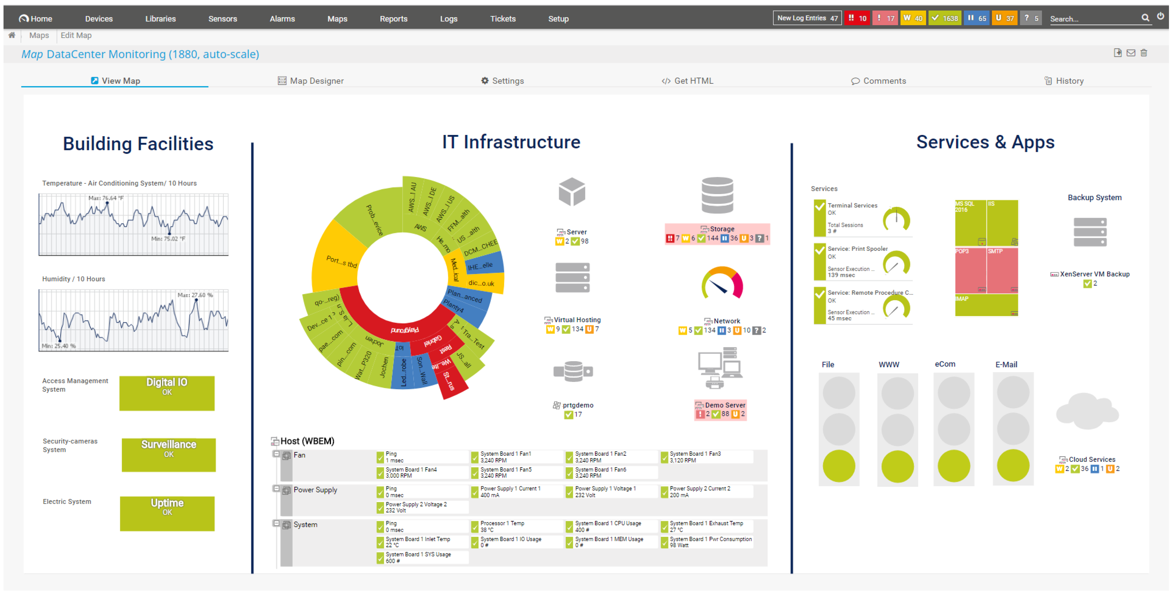
• The data are gathered from various sources such as logs, alarms, and other informational channels. The monitoring system plays a vital role in this process, cataloging defect occurrences and offering comprehensive data about these flaws. The collected data are then stored in a database system, paving the way for the crucial step of data analytics. This step encompasses advanced data analytics, data mining, machine learning, and cloud computing technologies. Data collection from network devices using a network monitoring program was carried out through the SNMP protocol.
• SNMP configuration on network devices: SNMP (simple network management protocol) is a standard network management protocol that allows network administrators to monitor and manage devices within a network. To collect data from network devices, SNMP was configured on each device. This involved setting SNMP parameters, such as the device address, the port used for SNMP, and the SNMP protocol version.
• Network monitoring program installation: After the configuration of SNMP on devices, a network monitoring program, which is PRTG network monitor in our case, was installed. It used the SNMP protocol to collect data from devices. The program can be installed on a computer or server located within the same network as network devices.
• Monitoring rule creation: Setting up monitoring rules allows determining which data need to be collected from each device within the network. In other words, the final training dataset consisted of feature matrix indicators collected by the monitoring system: CPU load, memory usage, temperature of network equipment components, network traffic, number of alarms, packet loss, and equipment availability. A binary vector of acceptable responses was created with a breakdown classification equal to 1 for normal equipment operation and equal to 0 otherwise.
• Monitoring initiation: After creating rules and starting the monitoring process, the PRTG network monitor collected and recorded data. Finally, data were saved in the program’s database.
• Data analysis: After data collection, analysis can be conducted using the monitoring program. The program can provide charts and diagrams that help analyze metric changes over time. Additionally, the program can alert potential network issues based on established metric threshold values. In our case, we limited ourselves to exporting data in “.csv” format for each individual network device.

3.2. Dataset

The observed network is a subset consisting of eight Layer 2 (L2) switches from a single vendor, which are part of a substantially larger deployed network. The dataset encompasses all TRAP messages generated by these devices from 12 December 2019 to 10 December 2020—a total of 363 days. These messages are aggregated into final log files in Comma Separated Values (CSV) format. After amalgamating the twelve-month logs from all eight switches, the resulting dataset contained 2923 entries, averaging 8 messages per day from each switch. Although this may be considered a modest data stream, it aligns with the expectations for a failure dataset, given that failures are inherently sporadic events. Each log adheres to a uniform format containing fourteen manually selected variables deemed relevant for the current research. These variables are:

• Date: The date on which the equipment status message was recorded. The date format used was “DD.MM.YYYY”, for example, “10.12.2020”. This column was subsequently removed as it did not offer any informative value.
• Uptime: The number of days the equipment functioned without any failures. The recorded format is numerical; for example, “95.00” indicates the switch operated for 95 consecutive days without interruptions or failures.
• Downtime: A metric denoting the period during which a specific switch or device in the network is either inaccessible or not functioning properly. This could occur due to various reasons, such as hardware failures, software bugs, or connectivity issues. The recorded format is percentage-based; for example, 0% indicates 24 h of uninterrupted operation, whereas 0.1% indicates a downtime of approximately 1–0.2% of a 24 h period, which equates to around 2 min.
• CPU load: The CPU load or utilization of the switch, recorded in a numerical format. For example, “8.12” signifies a CPU load of 81.2% of its full 100% capacity.
• CPU 1: In Catalyst 6500/6000 switches, there are two CPUs. One is the network management processor (NMP) or switch processor (SP), and the other is the multi-layer switch feature card (MSFC) or routing processor (RP). This entry captures the load on the Switch Processor (SP), which performs the following functions:
  • Participates in the learning and aging of MAC addresses. Note: MAC address learning is also known as path setup.
  • Initiates protocols and processes for network management, such as the spanning tree protocol (STP), Cisco discovery protocol (CDP), VLAN trunking protocol (VTP), dynamic trunking protocol (DTP), and port aggregation protocol (PAgP).
  • Handles network management traffic directed to the switch’s CPU, such as Telnet, HTTP, and SNMP traffic. The recorded format is numerical, for example, “8.76”.
• Available memory for Processor 1: This refers to the numerical value representing the available memory for Processor 1 at the time of measurement. The data are recorded in a numerical format, with the unit of measurement being megabytes (MB). For instance, a value of “52.00” signifies that 52 MB of memory is available for Processor 1.
• Percentage of available memory for Processor 1: This metric quantifies the availability of memory for Processor 1 as a percentage of the total 100%. The data are recorded in a percentage format, for example, “37%”, which indicates that 37% of the processor’s memory is available for computational tasks. During data preprocessing, the percentage symbol was removed because the predictive model was unable to interpret this character.
• Available memory for Processor 2: This metric presents data on the available memory for the second processor, recognizing that not all switches have dual processors. The routing processor (RP) performs several tasks:
  • Constructs and updates Layer 3 routing tables and the address resolution protocol (ARP).
  • Generates the forwarding information base (FIB) for Cisco express forwarding (CEF) and adjacency tables and loads them onto the policy feature card (PFC).
  • Manages network control traffic directed toward the RP, such as Telnet, HTTP, and SNMP traffic. The data are recorded in a numerical format, with the unit of measurement being megabytes (MB). For instance, a value of “1.73” signifies that 1.73 MB of memory is available for processing tasks.
• Percentage of available memory for Processor 2: This variable indicates the percentage of available memory for Processor 2 as a fraction of 100%. The data are recorded in a percentage format. For example, a value of “43%” signifies that 43% of the processor’s memory is available for task execution. During the data cleansing phase, the percentage symbol was removed due to incompatibilities with the predictive model.
• Overall available memory: This parameter measures the overall memory availability in percentage terms. For instance, a reading of “100%” implies that all of the memory or RAM capacity is available for utilization. The percentage symbol was removed during data preprocessing due to model limitations. Subsequently, the numerical value was simplified from 100 to 1 to facilitate data handling.
• Response time index (RTI): This is a metric employed to measure the response time of a network device or application. It serves as a vital indicator of the quality of service (QoS) within a network, particularly in scenarios where latency is a critical factor, such as voice or video conferencing. Response time is the duration between the sending of a request and the receipt of a corresponding response. This time encompasses network transmission delays, device processing delays, and other contributing factors. The RTI can be utilized for monitoring and analyzing network performance; a high RTI value may signal network issues that warrant investigation. The measurement format is numerical, recorded in milliseconds (ms). This metric captures the time required for a packet to travel from the sender to the receiver and back, and may include various types of delays such as transmission and processing delays. For example, a value of “70” would imply a 70-ms response time.
  • Optimal RTI: An RTI value of 20 ms is generally considered excellent for the majority of applications.
  • Average RTI: An RTI of 100 ms may be acceptable for certain types of traffic but could result in noticeable real-time delays for voice and video applications.
  • High RTI: If the RTI reaches 300 ms or more, this is likely indicative of significant network latency issues that could adversely impact the performance of network applications.
• CPU load index: This metric provides information reflecting the current load on the central processing unit (CPU). It is a quantitative assessment of the extent to which CPU time is being utilized and serves as an important indicator of overall device performance and health. In Cisco switches, the CPU load index is generally measured as a percentage ranging from 1% to 100%, where
  • 1–30%: This range is usually considered a normal load, indicating that the device is operating healthily.
  • 31–70%: This is a moderate load that may necessitate additional monitoring. It could be related to a temporary increase in traffic or a task consuming more resources.
  • 71–100%: This signifies a high or critical load, potentially indicating a problem. This could be due to misconfiguration, an attack, hardware defects, or other issues that could have a negative impact on the overall network operation.
• Traffic index: This metric is used for the quantitative assessment of the volume of traffic flowing through a switch over a specified period of time.
• Bandwidth analysis: This entails determining the data transfer rate through a specific port or interface of the switch. For instance, the traffic index might reveal that a certain port is being utilized at 70% of its maximum bandwidth capacity. In our context, data were recorded from TRUNK ports, which are channel ports connecting the switch to other network switches. The recording format is numerical. For example, a value of “9.32” means that the channel port operated at an average speed of 9.32 MB/s.
• Alarms: These are records from an alerting system designed to notify network administrators about various events, problems, or anomalous states that may require attention or intervention. The recording format is numerical. For example, “1” means that there was one alarm from the system, and “3” means there were three alarms from the system.
• Temperature: Most Cisco switches are equipped with built-in temperature sensors that continuously measure the temperature at various points within the device. In our case, the measurement format was numerical and in degrees Celsius, e.g., a reading of “42.0” signified that at the time of measurement, the equipment’s temperature was around 42 ${}^{\circ }$C. During data cleaning, the “${}^{\circ }$C” symbol was removed because the forecasting model could not interpret that symbol.

The raw monitoring data obtained during the export process requires processing to be used as a training dataset. The problem was that the data were exported in multiple CSV files and contained duplicate features with incorrect linguistic labels (see Figure 3). After processing the data, a feature matrix with dimensions [2] was obtained.

The resulting graph (see Figure 4) illustrates that not all criteria were important for predicting an event. The most important criteria were identified as “Alarms”, “CPU load”, “CPU1”, “Temperature”, “Traffic index”, “Response time index”, and “Available memory2” as the most significant factors affecting the final prediction outcome.

A split criterion was used in this study. The first step in building a decision tree is to determine the best attribute to split the data. This is typically done by using a measure of impurity like the Gini index [26,27] or information gain [27,28]. For example, information gain can be calculated as follows:

$$IG(S,A)=H\left(S\right)-\sum \frac{\left[S_v\right]}{S}\times H\left(S_v\right)$$

(1)

where

• $IG(S,A)$ is the information gain for attribute A on dataset T.
• $H\left(S\right)$ is the entropy of dataset T.
• $\left[S_v\right]$ is the number of samples in the subset $S_v$, created by splitting S on attribute A.
• $H\left(S_v\right)$ is the entropy of the subset $S_v$.

Then a stopping criteria has been established to prevent the decision tree from growing indefinitely. Some common stopping criteria include [29,30]:

• Maximum depth: The tree limit was 3 and 4;
• Minimum samples per node;
• Minimum information gain.

3.3. Pre-Modeling

In the initial stages of the research activity, an analysis of the input data was conducted utilizing the software suite RapidMiner Studio (version 10.0). The preliminary step involved the visualization of the input data. By uploading a pre-structured dataframe, it became possible to isolate the parameter requiring forecasting (see Figure 5). In our specific case, the criterion to be forecasted was the “breakage” of the switch (breaking).

Subsequently, the quick prototyping function was employed: Like many other data analysis tools, RapidMiner generates and tests various prototypes using all available machine learning algorithms in the library, based on the uploaded dataframe. In our case, nine different algorithms were tested in the “quick prototyping” mode:

• Logistic regression.
• Random forest.
• Gradient boosted trees.
• SVM (support vector machine).
• Naïve Bayes.
• kNN (k-nearest neighbor).
• Linear regression.
• Gradient boosted regression.
• Neural network.

As a result of the prototyping, an algorithm was identified that demonstrated the highest applicability in relation to the input data. The most positive preliminary results were produced by decision tree algorithms, random forest, SVM, and kNN. These algorithms exhibited over 60% accuracy in preliminary failure prediction and had shorter training times compared to other types of algorithms.

The algorithms in question come with specific hyperparameters that require tuning, usually essential for empirical adjustment. Since they all belong to the same environment, various evaluations concerning training time or memory usage can be carried out. Additionally, there is the flexibility to employ a unified dataset format for all algorithms. Based on the prototyping results, it was decided to conduct a more thorough test of the random forest algorithm and the decision tree algorithm with cross-validation, using the same RapidMiner Studio software.

Initially, a model was constructed where an input dataset consisting of approximately 1800 records was loaded. Subsequently, attributes were selected, roles were assigned, and cross-validation was performed. The ratio of test to training blocks was 40 to 60; i.e., the model was trained on 60% of the data and made forecasts on the remaining 40%. To ensure a reliable model evaluation, a 5-fold cross-validation was used, although this could be increased to 15–20 folds. However, some events have a reduced number of positive samples, which might result in some folds having few or no positive samples, making it impossible to calculate some metrics. The model’s workflow is illustrated in Figure 6.

The outcome of this model verification showed an accuracy of 99.84%, but the recall rate was 72.73%. Such a high percentage of predictive accuracy indicated that the chosen strategy was correct, but required some fine-tuning as the system predicted three false negatives (see Figure 7), which is unacceptable in our scenario.

In light of the above, we implemented the following changes to the model to improve output metrics: we added data from three additional switches, increasing the total number of input records to 2900, and raised the number of cross-validation folds from 5 to 20 while maintaining the 60/40 training-to-test block ratio. As a result of these changes, there was a qualitative improvement in the final forecasts, as shown in Figure 7 and Figure 8. The accuracy metric increased to 99.97%, and the recall for failure prediction rose to 99%, as indicated in Figure 8 Nonetheless, the time for training and prediction increased proportionally, from an average of 4 s to around 11–12 s (see Figure 8).

3.4. Proposed Model

Decision trees are used in our study. Figure 9 illustrates its use in order to predict network equipment failures.

Decision trees are prone to overfitting, which means they can grow indefinitely if not constrained. To prevent decision trees from growing too complex and overfitting the training data, various criteria and techniques are used to determine when to stop or prune the tree. Here are the main criteria used to prevent decision trees from growing indefinitely:

• Maximum depth (max depth): Setting a maximum depth for the decision tree restricts how many levels it can grow. If a tree reaches this depth during construction, it stops splitting and becomes a leaf node. This helps prevent overfitting by limiting the tree’s complexity.
• Minimum samples per leaf: This criterion specifies the minimum number of samples required in a leaf node. If a node has fewer samples than this threshold after a split, the split is not allowed. It prevents the creation of very small leaf nodes, which can capture noise in the data.
• Minimum samples per split: Similar to the minimum samples per leaf, this criterion specifies a minimum number of samples required to perform a split at a node. If there are fewer samples than this threshold, the split is not considered, preventing further growth of the tree on small subsets of data.
• Maximum features: This parameter limits the number of features considered for each split. It can be set to a fixed number or a percentage of total features. Limiting the features considered at each node helps control tree complexity and prevents overfitting.
• Impurity threshold (minimum impurity decrease): Nodes are split only if the impurity decrease (e.g., Gini impurity or entropy) resulting from the split exceeds a certain threshold. If the decrease in impurity is below this threshold, the split is not performed, which helps avoid splitting into noisy or irrelevant features.
• Pruning techniques: After growing a full tree, pruning techniques can be applied to remove branches that do not contribute significantly to improving predictive accuracy. Pruning involves evaluating the impact of removing subtrees and keeping only those that improve the tree’s generalization performance on validation data.
• Cross-validation: Cross-validation techniques, such as k-fold cross-validation, can be used to estimate the optimal tree depth and other hyperparameters by assessing a tree’s performance on different validation subsets of the data. This helps find the right trade-off between model complexity and predictive accuracy.

These criteria and techniques are essential for preventing decision trees from growing indefinitely and, instead, ensuring that they generalize well to unseen data. The goal is to strike a balance between capturing useful patterns in the data and avoiding the inclusion of noise or overfitting, which can lead to poor model performance on new data. In our study, we used the mentioned criteria in our scripts in order to prevent decision trees from growing too complex and overfitting.

In the next step, SVM is used to predict the LAN switches failures. In order to use SVM to predict LAN switch failures, some scripts are written. These scripts take the following points into consideration:

• The script starts by importing several important Python libraries used for data manipulation, visualization, and machine learning (Python libraries, such as numpy, pandas, sklearn, and matplotlib).
• Data loading: The authors take some of the collected data from the monitoring systems and prepare them for further manipulation. The next step is “data preprocessing”:

  (a)

  The authors add comments within triple quotes to avoid overlapping histograms for each specified feature. This allows for a comparison of distributions in cases where ’Breaking’ is ’Yes’ or ’No’.

  (b)

  Conversion to binary: The ’Breaking’ column is the target variable, and it is converted from ’Yes’/’No’ to a binary format (1/0) using a dictionary mapping.

  (c)

  Feature selection: Some columns are dropped from the DataFrame “ds” (as specified in cat_ feet), and the modified DataFrame only contains numerical features.

• Train–test split: The dataset is split into a training set (X_ train, Y_ train) and a test set (X_ test, Y_ test). The test set size is set to 50% of the total data. The random_ state=0 ensures that the splits are reproducible.
• Modeling. A pipeline is created with two steps:

  (a)

  “StandardScaler()”: Standardization of a dataset is a common requirement for many machine learning estimators. It standardizes features by removing the mean and scaling to unit variance.

  (b)

  “SVC(gamma=’auto’, probability=True)”: SVC stands for support vector classification, which is a type of SVM. By setting “gamma=’auto’”, the gamma parameter is set to 1/n_ features. Setting “probability=True” enables the classifier to provide probability estimates. After all, the pipeline is fitted on the training data.

• Prediction: Predictions (“clf_ pred”) are made on the test data. Probabilities (“clf_ pred_ proba”) are also calculated for each prediction. This is possible because “probability=True” is set in the SVC classifier.
• Model evaluation: Several metrics are printed out for evaluating the model:

  (a)

  Accuracy: This is the percentage of correct predictions. It is calculated using “accuracy_ score(clf_ pred, Y_ test)”, comparing the predicted values against the actual values from the test set.

  (b)

  Cross-validation score: This is another way to measure the effectiveness of the trained model, which works by dividing the dataset into “k” groups or folds, repeatedly training the model on k-1 folds while evaluating it on the held-out fold.

  (c)

  Classification report: This report displays the precision, recall, F1-score, and support for the model.

• Alerts: Finally, the script prints “Alarm!” for every instance in the test set that is predicted as class 1 (“Breaking” = Yes). This could be interpreted as an alert system where an alarm is raised if the model predicts a system failure.

These steps were used for LAN switch failure prediction with SVM. The specific implementation details and library choice may vary, depending on the programming language and tools.

3.5. Results and Discussion

In this dataset, a machine learning algorithm was applied, specifically the random forest method, which successfully classified the impending network equipment failure with an accuracy of 98.3%. The SVC method also successfully classified the impending network equipment failure with an accuracy of 94.28% (see Figure 10).

When comparing two prediction methods (Figure 10, Figure 11 and Figure 12), a significant influence of the input parameters on the success of the prediction was revealed, such as “Alarms”, “CPU load”, “Traffic index”, “Temperature”, and a negligible influence of all other input parameters. This is a clear indication that out of 14 parameters, only 5–6 are important for the prediction system. In turn, this implies a more optimal methodology for collecting data from monitoring systems. It should also be emphasized that the SVC model was trained and tested on significantly fewer data compared to the random forest model: 116 rows of records versus 2503.

It can be observed that there were no major differences in prediction outcomes when comparing the methods using a histogram (as shown in Figure 11). However, there is a notable disparity in the processing time: The SVC method requires 10–25% more time to analyze the same volume of data. This difference in the processing time may seem minimal, but it is significant when applied to larger, industrial-scale data networks that necessitate real-time data analysis. In scenarios where networks may have up to 200 switches, even marginal increases in processing time can translate into considerable inefficiencies.

Finally, one can see a difference in the prediction accuracy (Figure 10). The tree-based models consistently delivered a prediction accuracy of $99.39\%$, whereas the SVC model yielded a slightly lower accuracy of $94.28\%$. This discrepancy in accuracy, while potentially minor, could have significant consequences in large-scale industrial applications where high precision is required.

The high accuracy achieved by the decision tree and support vector machine (SVM) models for LAN failure prediction involves understanding the factors that contribute to their effectiveness in this specific context. We start by highlighting the importance of selecting relevant features or network parameters for LAN failure prediction. The chosen features provide critical information about network health and performance, allowing the models to identify patterns that are indicative of potential failures. In addition, decision trees are capable of capturing complex relationships between the selected features. We emphasize that the tree structure enables the model to divide the feature space into subsets that represent different LAN states or failure conditions. However, SVM uses kernel functions. SVMs can effectively map the input features into a higher-dimensional space, making it easier to separate LAN failure instances from non-failure instances. In the other side, the decision tree model offers interpretability, making it easier to understand why certain decisions or splits are made. This can help network administrators gain insights into the specific network parameters that contribute to failure predictions. Both models exhibit strong generalization capabilities. They have learned from historical LAN data, enabling them to identify similar patterns in unseen data. This generalization is a key factor in their high accuracy when applied to new LAN scenarios. Furthermore, SVM is a flexible model that can handle both linear and non-linear relationships in the data. This adaptability allows it to capture a wide range of LAN failure patterns, making it suitable for various network configurations. Finally, while the models have demonstrated high accuracy, there is always room for improvement. Ongoing data collection and model refinement can further enhance their predictive capabilities.

The point at which an increase in data volume no longer significantly enhances prediction accuracy, when using decision trees and SVM for LAN failure prediction, can be described by the concept of diminishing returns. Initially, as the volume of training data increases, both algorithms benefit from more diverse examples and patterns to learn from, leading to improved accuracy. However, there comes a point where the marginal gain in accuracy levels off, and adding more data becomes less impactful. This threshold depends on factors such as the complexity of the LAN environment, the richness of the feature set, and the inherent noise in the data. Beyond this point, additional data may introduce more noise or redundant information, making it more challenging for the models to extract meaningful insights. Hence, it is essential to carefully monitor and evaluate model performance in relation to data volume to determine the optimal dataset size that balances accuracy gains with computational resources and data management constraints.

The study’s findings, which demonstrate the accurate prediction of LAN equipment failures using machine learning algorithms (decision trees and SVM), have profound implications for real-world network management and communication network performance. By accurately forecasting LAN equipment failures, network administrators and organizations can realize several tangible benefits. For instance accurate prediction enables proactive maintenance and timely interventions to prevent or mitigate equipment failures. This, in turn, significantly reduces network downtime and service disruptions. A well-maintained network experiences fewer outages, leading to enhanced reliability and minimal impact on end-users or critical business operations. Furthermore, minimizing network downtime not only improves operational efficiency but also translates into cost savings. Organizations no longer need to allocate extensive resources for emergency repairs or costly hardware replacements. Predictive maintenance allows for planned and cost-effective equipment replacements or repairs. In addition, accurate failure prediction empowers network administrators to proactively manage and optimize network resources. They can allocate bandwidth, allocate network assets, and fine-tune configurations based on predicted failures or potential traffic shifts, ensuring that network performance is consistently optimized. On the other hand, a reliable network with minimal downtime results in a consistently positive user experience. This is especially critical for organizations that rely on real-time applications, such as video conferencing, VoIP, and cloud services. Accurate failure prediction ensures that users can access services without interruptions or latency issues, ultimately improving customer satisfaction and employee productivity. Finally, knowing when and where equipment failures are likely to occur allows organizations to allocate resources more effectively. They can maintain an adequate inventory of replacement parts or equipment, reducing delays in restoring network functionality.

4. Conclusions

LAN failure prediction could represent a significant advancement in the field of network management and reliability. Decision trees and support vector machines (SVMs) have been used in our study for LAN failure prediction. Both algorithms have demonstrated their efficacy in accurately forecasting LAN equipment failures, offering valuable insights and benefits to organizations and network administrators. It has been found that LAN equipment failure prediction is instrumental in fostering a more reliable, efficient, and cost-effective communication network infrastructure. These predictions have a direct impact on reducing downtime, improving network management practices, enhancing user experiences, and optimizing resource allocation, ultimately leading to improved overall network performance in real-world scenarios.

Future work on the practical implementation of LAN failure prediction using machine learning will likely focus on refining predictive models with more extensive datasets and exploring emerging techniques. Additionally, the integration of predictive maintenance systems into network infrastructure management tools will be a crucial area of development, allowing organizations to seamlessly incorporate machine learning-driven predictions into their daily network operations.

References

1. Potapov, V.I.; Shafeeva, O.P.; Doroshenko, M.S.; Chervenchuk, I.V.; Gritsay, A.S. Numerically-analytical solution of problem gaming confrontation hardware-redundant dynamic system with the enemy operating in conditions of incomplete information about the behavior of participants in the game. J. Phys. Conf. Ser. 2018, 1050, 012062. [Google Scholar] [CrossRef]
2. Storozhenko, N.R.; Goleva, A.I.; Tunkov, D.A.; Potapov, V.I. Modern problems of information systems and data networks: Choice of network equipment, monitoring and detecting deviations and faults. J. Phys. Conf. Ser. 2020, 1546, 012030. [Google Scholar] [CrossRef]
3. Cybersecurity Threatscape 2019 (No Date) Ptsecurity.com. Available online: Https://www.ptsecurity.com/ww-en/analytics/cybersecurity-threatscape-2019/ (accessed on 19 August 2023).
4. Juliono, A.; Rosyani, P. Implementasi Sistem Monitoring Jaringan Internet Kantor PT. Permodalan Nasional Madani (Persero) Menggunakan Jessie Observium Dan Mikrotik (Simonjangkar). Kernel J. Ris. Inov. Bid. Inform. Pendidik. Inform. 2022, 3, 27–32. [Google Scholar]
5. Josephsen, D. Building a Monitoring Infrastructure with Nagios; Prentice Hall PTR: Indianapolis, IN, USA, 2007. [Google Scholar]
6. Zhou, J.; Huang, H.; Mattson, E.; Wang, H.F.; Haimson, B.C.; Doe, T.W.; Oldenburg, C.M.; Dobson, P.F. Modeling of hydraulic fracture propagation at the kISMET site using a fully coupled 3D network-flow and quasi-static discrete element model (No. INL/CON-17-41116). In Proceedings of the 42nd Workshop on Geothermal Reservoir Engineering Stanford University, Stanford, CA, USA, 13–15 February 2017. [Google Scholar]
7. Mistry, D.; Modi, P.; Deokule, K.; Patel, A.; Patki, H.; Abuzaghleh, O. Network traffic measurement and analysis. In Proceedings of the 2016 IEEE Long Island Systems, Applications and Technology Conference (LISAT), Farmingdale, NY, USA, 29 April 2016; pp. 1–7. [Google Scholar]
8. Olups, R. Zabbix 1.8 Network Monitoring; Packt Publishing Ltd.: Birmingham, UK, 2010. [Google Scholar]
9. Orazbayev, B.; Ospanov, Y.; Orazbayeva, K.; Makhatova, V.; Kurmangaziyeva, L.; Utenova, B.; Mailybayeva, A.; Mukatayev, N.; Toleuov, T.; Tukpatova, A. System Concept for Modelling of Technological Systems and Decision Making in Their Management; PC Technology Center: Kharkiv, Ukraine, 2021; 180p. [Google Scholar] [CrossRef]
10. Sansyzbay, L.Z.; Orazbayev, B.B. Modeling the operation of climate control system in premises based on fuzzy controller. J. Phys. Conf. Ser. 2019, 1399, 044017. [Google Scholar] [CrossRef]
11. Shao, J.; Zhao, Z.; Yang, L.; Song, P. Remote Monitoring and Control System Oriented to the Textile Enterprise. In Proceedings of the 2009 Second International Symposium on Knowledge Acquisition and Modeling, Wuhan, China, 30 November–1 December 2009; Volume 3, pp. 151–154. [Google Scholar]
12. Li, Q.; Yang, Y.; Jiang, P. Remote Monitoring and Maintenance for Equipment and Production Lines on Industrial Internet: A Literature Review. Machines 2022, 11, 12. [Google Scholar] [CrossRef]
13. Yugapriya, M.; Judeson, A.K.J.; Jayanthy, S. Predictive Maintenance of Hydraulic System using Machine Learning Algorithms. In Proceedings of the 2022 International Conference on Electronics and Renewable Systems (ICEARS), Tuticorin, India, 16–18 March 2022; pp. 1208–1214. [Google Scholar]
14. Dsouza, J.; Velan, S. Preventive maintenance for fault detection in transfer nodes using machine learning. In Proceedings of the 2019 International Conference on Computational Intelligence and Knowledge Economy (ICCIKE), Dubai, United Arab Emirates, 11–12 December 2019; pp. 401–404. [Google Scholar]
15. Polat, H.; Polat, O.; Cetin, A. Detecting DDoS attacks in software-defined networks through feature selection methods and machine learning models. Sustainability 2020, 12, 1035. [Google Scholar] [CrossRef]
16. Wang, M.; Cui, Y.; Wang, X.; Xiao, S.; Jiang, J. Machine learning for networking: Workflow, advances and opportunities. IEEE Netw. 2017, 32, 92–99. [Google Scholar] [CrossRef]
17. Jinglong, Z.; Changzhan, H.; Xiangming, W.; Jiakun, A.; Chunguang, H.; Jinglin, H. Research on Fault Prediction of Distribution Network Based on Large Data. In MATEC Web of Conferences; EDP Sciences: Ulys, France, 2017; Volume 139, p. 00149. [Google Scholar]
18. Le, T.; Luo, M.; Zhou, J.; Chan, H.L. Predictive maintenance decision using statistical linear regression and kernel methods. In Proceedings of the 2014 IEEE Emerging Technology and Factory Automation (ETFA), Barcelona, Spain, 16–19 September 2014; pp. 1–6. [Google Scholar]
19. Harrell, F.E. Regression Modeling Strategies: With Applications to Linear Models, Logistic Regression, and Survival Analysis; Springer: New York, NY, USA, 2001; Volume 608. [Google Scholar]
20. Liu, T.; Wang, S.; Wu, S.; Ma, J.; Lu, Y. Predication of wireless communication failure in grid metering automation system based on logistic regression model. In Proceedings of the 2014 China International Conference on Electricity Distribution (CICED), Shenzhen, China, 23–26 September 2014; pp. 894–897. [Google Scholar]
21. Fletcher, S.; Islam, M.Z. Decision tree classification with differential privacy: A survey. Acm Comput. Surv. (CSUR) 2019, 52, 1–33. [Google Scholar] [CrossRef]
22. Priyanka; Kumar, D. Decision tree classifier: A detailed survey. Int. J. Inf. Decis. Sci. 2020, 12, 246–269. [Google Scholar] [CrossRef]
23. Mohammadi, M.; Rashid, T.A.; Karim, S.H.T.; Aldalwie, A.H.M.; Tho, Q.T.; Bidaki, M.; Rahmani, A.M.; Hosseinzadeh, M. A comprehensive survey and taxonomy of the SVM-based intrusion detection systems. J. Netw. Comput. Appl. 2021, 178, 102983. [Google Scholar] [CrossRef]
24. Cervantes, J.; Garcia-Lamont, F.; Rodríguez-Mazahua, L.; Lopez, A. A comprehensive survey on support vector machine classification: Applications, challenges and trends. Neurocomputing 2020, 408, 189–215. [Google Scholar] [CrossRef]
25. Myrzatay, A.; Rzayeva, L. Creation of Forecast Algorithm for Networking Hardware Malfunction in the context of small number of breakdowns. Int. J. Eng. Res. Technol. 2020, 13, 1243. [Google Scholar] [CrossRef]
26. Bouke, M.A.; Abdullah, A.; ALshatebi, S.H.; Abdullah, M.T.; El Atigh, H. An intelligent DDoS attack detection tree-based model using Gini index feature selection method. Microprocess. Microsyst. 2023, 98, 104823. [Google Scholar] [CrossRef]
27. Kent, J.T. Information gain and a general measure of correlation. Biometrika 1983, 70, 163–173. [Google Scholar] [CrossRef]
28. Englezou, Y.; Waite, T.W.; Woods, D.C. Approximate Laplace importance sampling for the estimation of expected Shannon information gain in high-dimensional Bayesian design for nonlinear models. Stat. Comput. 2022, 32, 82. [Google Scholar] [CrossRef]
29. Rokach, L.; Maimon, O. Decision trees. In Data Mining and Knowledge Discovery Handbook; Springer: New York, NY, USA, 2005; pp. 165–192. [Google Scholar]
30. Costa, V.G.; Pedreira, C.E. Recent advances in decision trees: An updated survey. Artif. Intell. Rev. 2023, 56, 4765–4800. [Google Scholar] [CrossRef]
Figure 1. Example of the PRTG network monitoring system information panel.
Electronics 12 03950 g001
Figure 2. Example of LAN devices interconnected in a star topology.
Electronics 12 03950 g002
Figure 3. Training dataset after transformation.
Electronics 12 03950 g003
Figure 4. Key features of the model and their corresponding weight in the forecasting system.
Electronics 12 03950 g004
Figure 5. Visualization of data loaded into the model.
Electronics 12 03950 g005
Figure 6. Prediction model built in the RapidMiner software.
Electronics 12 03950 g006
Figure 7. Model results.
Electronics 12 03950 g007
Figure 8. Results of the improved model.
Electronics 12 03950 g008
Figure 9. Decision tree for network equipment failure prediction.
Electronics 12 03950 g009
Figure 10. SVC, RF, and DT model accuracy results.
Electronics 12 03950 g010
Figure 11. Dependencies of input parameters for the failure prediction on SVC.
Electronics 12 03950 g011
Figure 12. Comparing both models by temperature data array.
Electronics 12 03950 g012
Disclaimer/Publisher’s Note: The statements, opinions and data contained in all publications are solely those of the individual author(s) and contributor(s) and not of MDPI and/or the editor(s). MDPI and/or the editor(s) disclaim responsibility for any injury to people or property resulting from any ideas, methods, instructions or products referred to in the content.