
Robust Adaptive Beamforming Algorithm Based on Complex Gauss–Legendre Integral


Abstract
:1. Introduction
2. Data Model
3. Algorithms
3.1. Interference Noise Covariance Matrix Reconstruction
3.2. Steering Vector Correction
| Algorithm 1 The proposed covariance matrix reconstruction and steering vector estimation |
|
4. Simulation
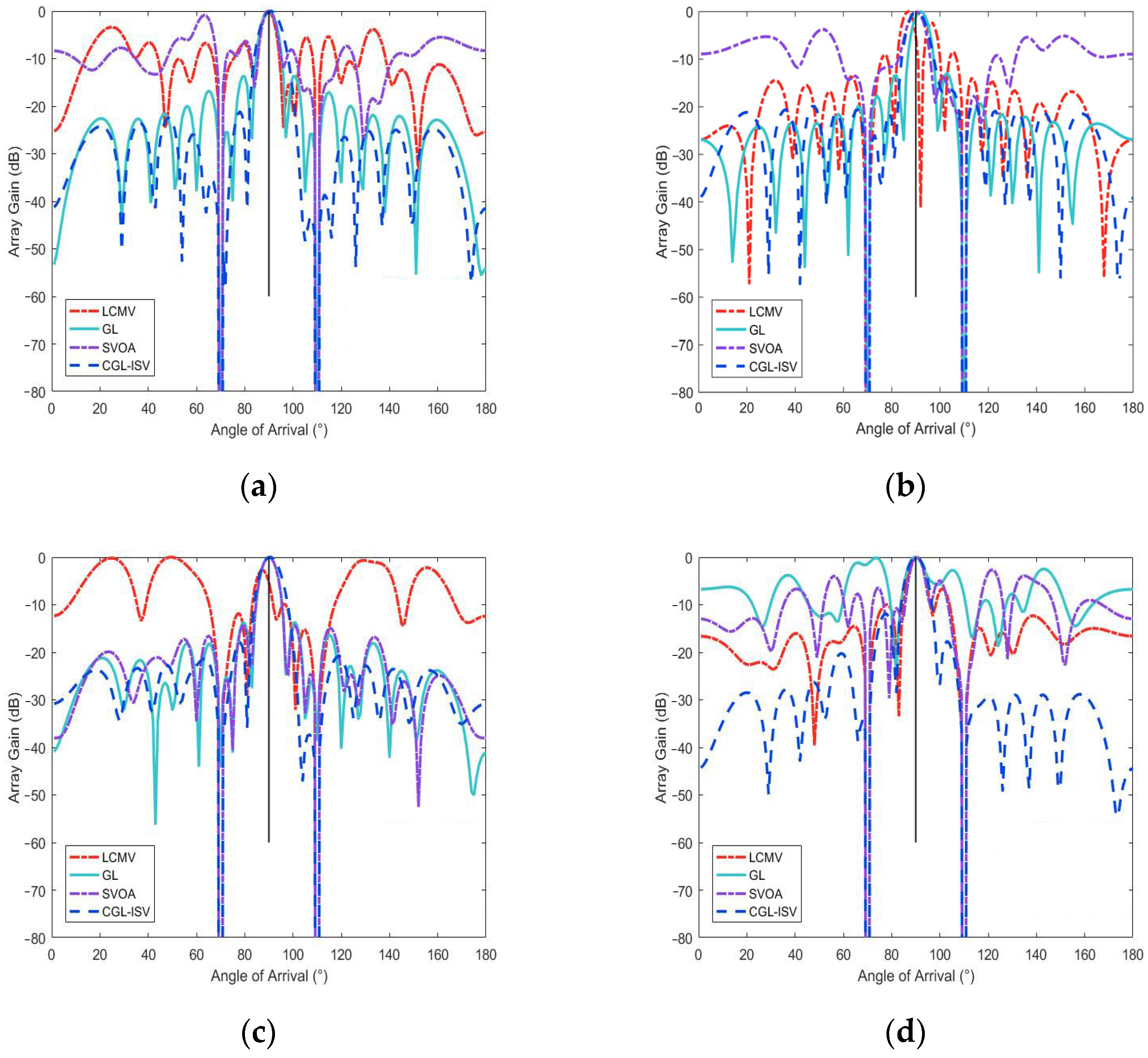
- Beampattern: For the far-field signal with THE Direction Of Arrival (DOA) and steering vector , the array outputs ARE . The array output is given by . According to the definition of the beampattern function, the expression of beampattern function is shown as follows:
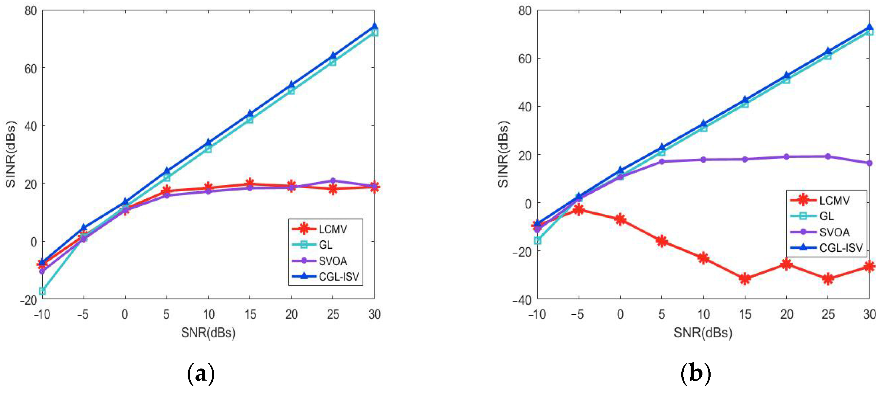
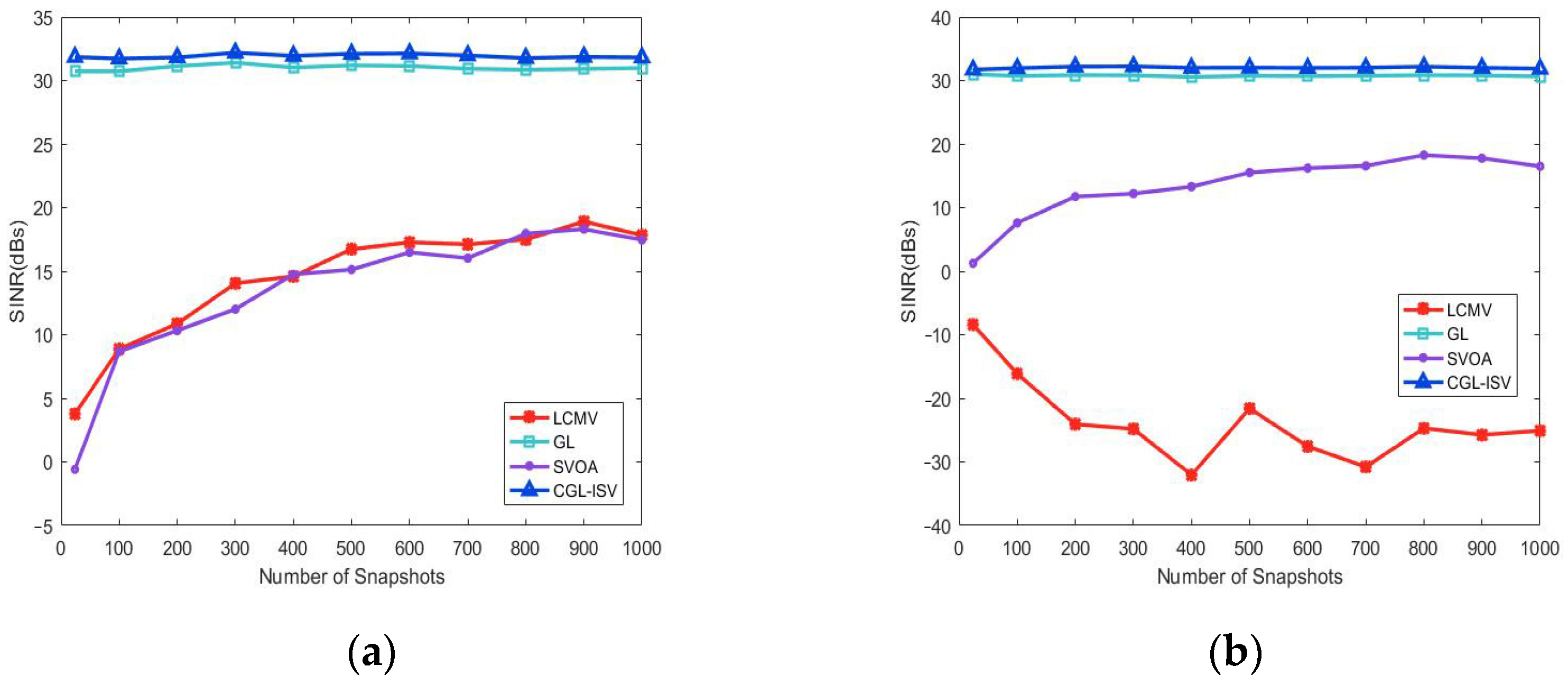
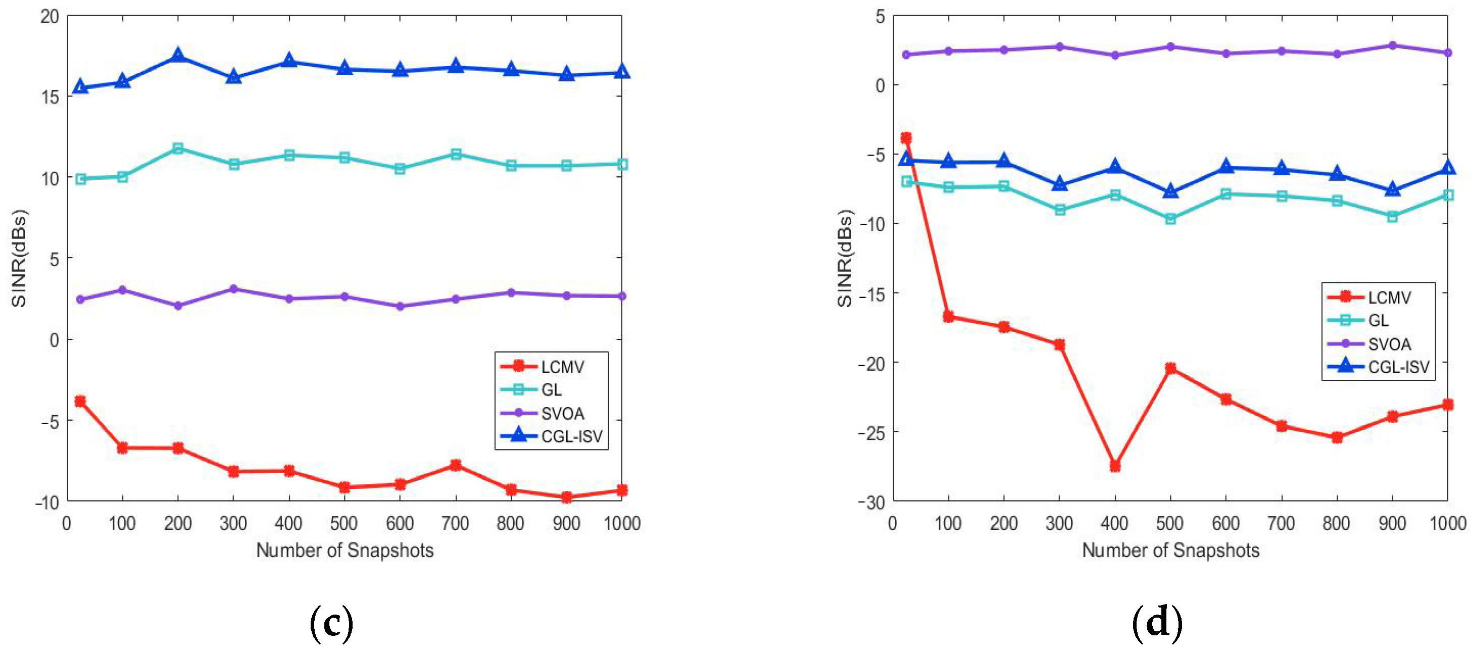
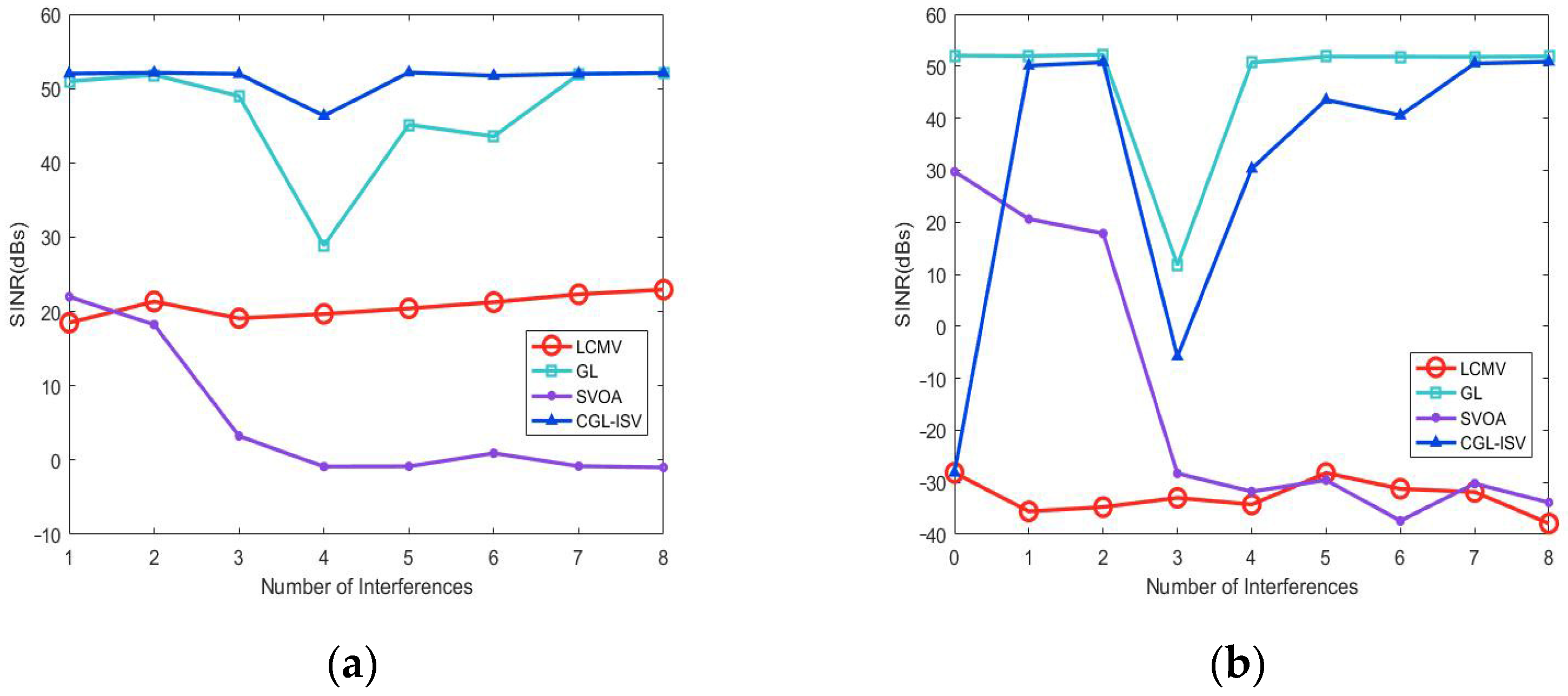
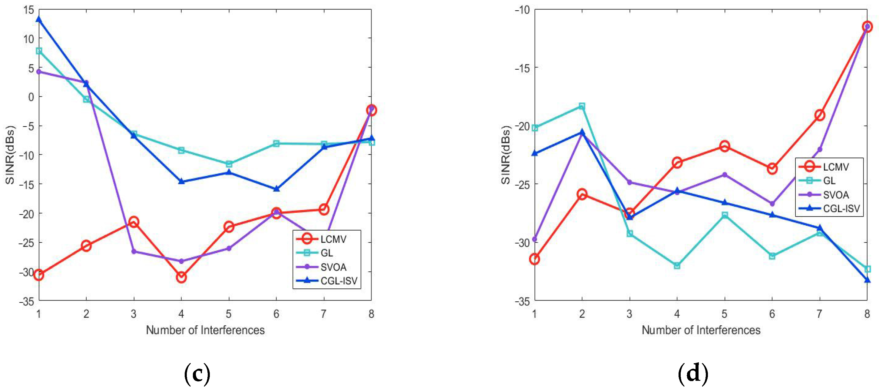
- Output SINR: For an adaptive antenna array system, the output SINR is defined as the output signal power divided by the output interference-and-noise power. Normally, the dB is employed as the unit of the output SINR and is given bywhere is the covariance matrix of the desired signal, and is the covariance matrix of the interference-and-noise.
4.1. The Beam Patterns
4.2. The Patterns of SINR with SNR
4.3. The Patterns of SINR with Snapshots
4.4. The Patterns of SINR with Interferences
5. Conclusions
Author Contributions
Funding
Data Availability Statement
Conflicts of Interest
References
- Saeed, M.; Osman, K. Robust adaptive beamforming for fast moving interference based on the covariance matrix reconstruction. IET Signal Process. 2019, 13, 486–493. [Google Scholar]
- Alon, A.; Miriam, D. A linearly constrained minimum variance beamformer with a pre-specified suppression level over a pre-defined broad null sector. Signal Process. 2015, 109, 165–171. [Google Scholar]
- Zhao, Y.; Li, W.X.; Mao, X.J.; Zhang, N. A beamforming null broadening method to resist array flow pattern error. J. Harbin Eng. Univ. 2018, 39, 163–168. [Google Scholar]
- Dang, J.; Zhang, Z.C.; Wu, L. Joint Beamforming for Intelligent Reflecting Surface Aided Wireless Communication Using Statistical CSI. China Commun. 2020, 17, 147–157. [Google Scholar] [CrossRef]
- Carlson, B.D. Covariance matrix estimation errors and diagonal loading in adaptive arrays. China Commun. 1988, 21, 397–401. [Google Scholar] [CrossRef]
- Elnashar, A.; Elnoubi, S.M.; El-Mikati, H.A. Further study on robust adaptive beamforming with optimum diagonal loading. IEEE Trans. Antennas Propag. 2006, 54, 3647–3658. [Google Scholar] [CrossRef]
- Du, L.; Li, J.; Stoica, P. Fully automatic computation of diagonal loading levels for robust adaptive beamforming. IEEE Trans. Aerosp. Electron. Syst. 2010, 46, 449–458. [Google Scholar] [CrossRef]
- Gu, Y.; Leshem, A. Robust adaptive beamforming based on interference covariance matrix reconstruction and steering vector. IEEE Trans. Signal Process. 2012, 60, 3881–3885. [Google Scholar]
- Duan, Y.; Gong, Y.; Yang, X.; Gao, W. Oblique Projection-Based Covariance Matrix Reconstruction and Steering Vector Estimation for Robust Adaptive Beamforming. Electronics 2022, 11, 3478. [Google Scholar] [CrossRef]
- Feldman, D.D. An analysis of the projection method for robust adaptive beamforming. IEEE Trans. Antennas Propag. 1996, 44, 1023–1030. [Google Scholar] [CrossRef]
- Huang, F.; Sheng, W.; Ma, X. Modified projection approach for robust adaptive array beamforming. Signal Process. 2012, 92, 1758–1763. [Google Scholar] [CrossRef]
- Jia, W.; Jin, W.; Zhou, S.; Yao, M. Robust adaptive beamforming based on a new steering vector estimation algorithm. Signal Process. 2013, 93, 2539–2542. [Google Scholar] [CrossRef]
- Li, J.; Stoicaand, P.; Wang, Z. on robust Capon beamforming and diagonal loading. IEEE Trans. Signal Process. 2003, 51, 1702–1715. [Google Scholar] [CrossRef]
- Khabbazibasmenj, A.; Vorobyov, S.A.; Hassanien, A. Robust adaptive beamforming based on steering vector estimation with as little as possible prior information. IEEE Trans. Signal Process. 2012, 60, 2974–2987. [Google Scholar] [CrossRef]
- Fan, Z.; Liang, G.L.; Wang, Y.L. A zero-trap broadening robust adaptive beamforming algorithm. J. Electron. Inf. Technol. 2013, 35, 2764–2770. [Google Scholar] [CrossRef]


Disclaimer/Publisher’s Note: The statements, opinions and data contained in all publications are solely those of the individual author(s) and contributor(s) and not of MDPI and/or the editor(s). MDPI and/or the editor(s) disclaim responsibility for any injury to people or property resulting from any ideas, methods, instructions or products referred to in the content. |
© 2023 by the authors. Licensee MDPI, Basel, Switzerland. This article is an open access article distributed under the terms and conditions of the Creative Commons Attribution (CC BY) license (https://creativecommons.org/licenses/by/4.0/).
Share and Cite
Cui, L.; Xue, K.; Wang, B.; Zhang, Y. Robust Adaptive Beamforming Algorithm Based on Complex Gauss–Legendre Integral. Electronics 2023, 12, 3794. https://doi.org/10.3390/electronics12183794
Cui L, Xue K, Wang B, Zhang Y. Robust Adaptive Beamforming Algorithm Based on Complex Gauss–Legendre Integral. Electronics. 2023; 12(18):3794. https://doi.org/10.3390/electronics12183794
Chicago/Turabian StyleCui, Lin, Kai Xue, Boyan Wang, and Yuanbang Zhang. 2023. "Robust Adaptive Beamforming Algorithm Based on Complex Gauss–Legendre Integral" Electronics 12, no. 18: 3794. https://doi.org/10.3390/electronics12183794
APA StyleCui, L., Xue, K., Wang, B., & Zhang, Y. (2023). Robust Adaptive Beamforming Algorithm Based on Complex Gauss–Legendre Integral. Electronics, 12(18), 3794. https://doi.org/10.3390/electronics12183794