An Off-Line Error Compensation Method for Absolute Positioning Accuracy of Industrial Robots Based on Differential Evolution and Deep Belief Networks

Abstract

Industrial robots have been increasingly used in the field of intelligent manufacturing. The low absolute positioning accuracy of industrial robots is one of the difficulties in their application. In this paper, an accuracy compensation algorithm for the absolute positioning of industrial robots is proposed based on deep belief networks using an off-line compensation method. A differential evolution algorithm is presented to optimize the networks. Combined with the evidence theory, a position error mapping model is proposed to realize the absolute positioning accuracy compensation of industrial robots. Experiments were conducted using a laser tracker AT901-B on an industrial robot KR6_R700 sixx_CR. The absolute position error of the end of the robot was reduced from 0.469 mm to 0.084 mm, improving the accuracy by 82.14% after the compensation. Experimental results demonstrated that the proposed compensation algorithm could improve the absolute positioning accuracy of industrial robots, as well as its potential uses for precise operational tasks.

1. Introduction

Industry 4.0 technologies are critical and indispensable tools to propel social and technological innovation advancements. Previous research [1,2] noted that the use of Industry 4.0 technologies can better sustain current resources, reduce labor costs, be better sources of energy, and potentially produce higher-quality sustainable products. Examples of Industry 4.0 technologies include, but are not limited to, machine learning, virtual and augmented reality, IoT, artificial intelligence, big data, and robotics [3]. Ref. [4] found Industry 4.0 technologies assist manufacturing companies’ sustainability and increase their economic potential. Scholars have examined Industry 4.0 technologies in diverse industries besides manufacturing. Ref. [5] implemented a systematic review to understand the use of Industry 4.0 technologies in managing pandemics. The use of Industry 4.0 technologies to meet the increasing demands of society is ubiquitous; applications include robotics [6], artificial intelligence [7], IoT [8], augmented reality [9], big data [10], and machine learning [11] in food and agricultural sciences, to assist in more efficient and enhanced production, which is needed to feed a growing world population. Ref. [12] investigated the use of Industry 4.0 technologies in the manufacturing sector, as examined in 380 papers prior to 2020. Ref. [13] sought to understand the manufacturing patterns implemented based on Industry 4.0 technologies.

Modern advanced manufacturing technology and key technologies demonstrate the fundamental competitiveness of a nation’s manufacturing industry. Robotics is a significant Industry 4.0 innovation that offers immeasurable possibilities in manufacturing disciplines [14]. An industrial robot is a complex system that succeeds in situations involving cross-work environments, high repetition, and high-precision processing. The current manual-based processing methods cannot meet all the requirements of a short development cycle and high assembly precision [15], and the use of industrial robots for processing is an excellent solution to this problem. The repeat positioning accuracy of industrial robots during the actual work process is usually quite satisfactory [16], and is typically 0.1 mm. However, the absolute positioning accuracy is poor, with an accuracy range of only approximately 2–3 mm. The absolute positioning accuracy severely limits the promotion and application of industrial robots in the manufacturing industry.

To address the problem of poor absolute positioning accuracy at the end of industrial robots, scholars at home and abroad have proposed various solutions [17]. Kinematic model-based control of robot joints makes it possible to compensate for absolute positioning errors in industrial robots. However, the positioning accuracy of the robot is affected by the size of the error of each kinematic parameter. The kinematic parameter errors can be addressed using kinematic parameter identification. The resulting parameter errors can be applied to the kinematic model to realize the adjustment of the model. This increases the positioning accuracy of the robot in the actual working environment, and the generated kinematic errors can be used to upgrade the kinematic model. This improves the positioning accuracy requirements of robots in actual workplaces.

In addition to positioning errors caused by geometric factors, nongeometric factors, such as gear gap, joint deformation, and temperature change, also affect the end positioning accuracy of robots [18]. The error mechanisms affecting robot positioning accuracy are complex and interconnected [19]. It is difficult to establish an accurate kinematic model that can account for all sources of error. Researchers have begun to investigate the establishment of a mapping relationship between the theoretical and actual position values.

A co-kriging-based error compensation method [20] was suggested to improve the positioning accuracy of the aerial drilling robot. A compensation method based on error similarity and error correlation was proposed to increase the robot’s positioning accuracy [21]. First, the maximum working stiffness of the robotic drilling system in a specific machining task was obtained. This was achieved by optimizing the mounting angle between the motor spindle and the robot end flange. This optimization laid the groundwork for achieving high hole-processing accuracy. Second, the method for calculating the corresponding compensation value was introduced. This was undertaken according to the position to be drilled. The method took into account the force deformation at the robot end and the absolute positioning error of the robot [22]. Combining error similarity and a radial basis function (RBF) neural network, Wang [23] developed a position error compensation approach. The robot joint angle and position error were used to fit the experimental semi-variance function. The bandwidth of the RBF neural network was modified using the parameters of the semi-variance function. The position error of the target position was also estimated using the RBF neural network. The estimated position error was used to modify the target position to achieve the compensation effect. In precision manufacturing, Li [24] introduced a synchronization estimation approach for the total inertia and load torque of spindle-tool systems. The synchronization method was based on a novel double extended sliding mode observer (DESMO), which synchronously tracked the total inertia and load torque. The robustness of DESMO was enhanced by inserting a robust activator to reduce the effect of coupling errors between the two expansion terms. This was critical to the precision control of the spindle tool and directly influenced the control performance.

Long-term research has been carried out by Tian Wei’s team at the Nanjing University of Aeronautics and Astronautics to increase the absolute positioning accuracy of industrial robots. A robot positioning error compensation method based on a deep neural network [25] was proposed to perform Latin hypercube sampling in Cartesian space. A positioning error prediction model based on genetic particle swarm optimization and a deep neural network (GPSO-DNN) was developed to predict and compensate for positioning error. Then, a practical positioning error compensation scheme for mobile industrial robots was proposed [16]. A binocular vision measurement method for robot positioning was developed. A mapping model between theoretical and actual robot pose errors was proposed based on deep belief networks (DBN), and the pose error estimation was realized.

A method for optimizing neural networks using the genetic particle swarm algorithm was proposed. This was done to improve the positioning accuracy of robots [26]. The aim was to model and predict the positioning error of industrial robots and achieve the compensation of target points within the robot workspace. Tian [27] proposed an absolute positioning error compensation scheme based on the DBN and error similarity. Relevant scholars have conducted in-depth research. The accuracy and versatility of error prediction can be further studied to improve the absolute positioning accuracy of the robot [28]. In addition, there are many mathematical methods [29,30,31,32] that can also be used to study the positioning accuracy of robots. Analytic methods such as fractional order have gained more and more attention [33,34].

The DBN is simple in structure and is suitable for data training in industrial robots. The training time of the DBN is short, thereby helping to improve the efficiency of the robot. Meanwhile, the differential evolution (DE) algorithm is an optimization algorithm based on the theory of swarm intelligence. It has been widely used in many fields because of its simple principle, small number of controlled parameters, and strong robustness. Finally, evidence theory can make experimental results more reliable.

Min [35] proposed a stable and high-accuracy model-free calibration method for unopened robotic systems, which can significantly improve the robot positional accuracy. Ref. [36] proposed an adaptive hierarchical compensation method based on fixed-length memory window incremental learning and incremental model reconstruction. Real-time trajectory position error compensation technology that considers non-kinematic errors [37,38] has also been proposed.

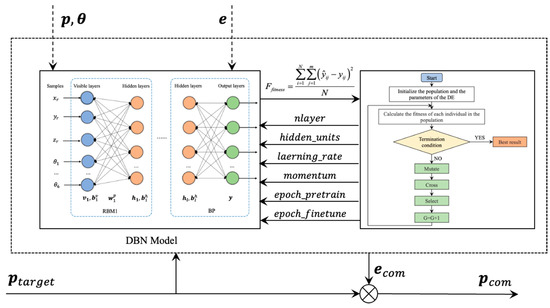
An absolute positioning accuracy compensation algorithm is proposed for industrial robots based on the DBN. The DE algorithm is used to optimize the DBN. The number of layer nodes, learning rate, momentum factor, restricted Boltzmann machine (RBM) iterations, and DBN fine-tuning iterations improve the optimization effect based on six dimensions and nine parameters. Combined with the evidence theory, the position error mapping model of industrial robots is established to realize its absolute positioning accuracy compensation. The technical process is shown in Figure 1.

Combined with the off-line feed-forward compensation method, the prediction error of the theoretical pose coordinates of the robot target is superimposed on the robot control instructions. The validity and superiority of the scheme are verified using a AT901-B laser tracker on KUKA KR6_R700 sixx_CR. The absolute positioning error at the end of the robot was reduced by 82.14%, from 0.469 mm to 0.084 mm. Future work can further consider industrial robot load, motion speed, acceleration, ambient temperature, or other factors that affect the absolute positioning accuracy of the robot.

The chapter arrangement of this paper is as follows: Section 1 serves as the introduction, providing an overview of the absolute positioning accuracy of industrial robots and the method proposed in this paper. Section 2 focuses on the robot positioning error prediction algorithm based on DE and DBN. Section 3 presents supervised predictive optimization based on evidence theory. Section 4 includes experimental setup, data collection, model training, and result analysis. Finally, Section 5 presents the conclusion.

2. Robot Positioning Error Prediction Algorithm Based on DE and DBN

2.1. Principle of the DBN

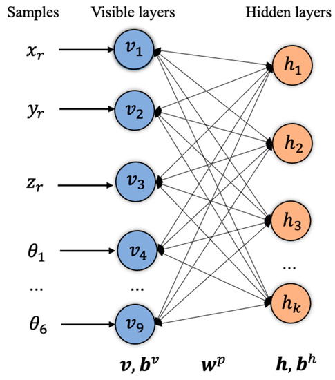
The DBN is a probabilistic generative model proposed by Geoffrey Hinton [39] in 2006. It is composed of multiple RBM connections and a regression layer, and created by fine-tuning the resulting deep network through gradient descent and back propagation (BP) to form the best model.

RBM, as the basic component of the DBN [40], is a generative random artificial neural network, which can learn probability distribution from the inputs. The structure of RBM is shown in Figure 2. RBM consists of two layers: the visible layer $\mathit{v}$ and the hidden layer $\mathit{h}$. The visible layer is used to receive training data. In this study, the visible layer is used to accept the desired position of the end in the robot coordinate system and the current robot joint angle. The input of the hidden layer is the output of the visible layer, which is used to extract features. The neurons of the two layers have intra-layer no-connection and inter-layer full-connection relationships. Between the visible and hidden layers is the weight matrix ${\mathit{w}}^p$. $\mathit{v}$ and $\mathit{h}$ represent the visible-layer and hidden-layer vectors, respectively, and $b^v$ and ${\mathit{b}}^h$ represent the biases of the visible and hidden layers, respectively.

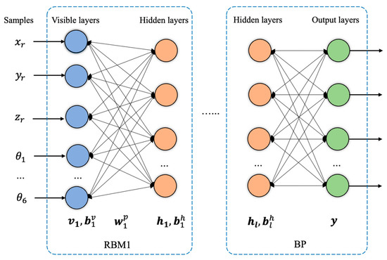
The multilayer RBM and the BP layer are stacked to form a DBN, as shown in Figure 3.

The first layer of RBM consists of a visible layer ${\mathit{v}}_1$ and a hidden layer ${\mathit{h}}_1$. The visible layer ${\mathit{v}}_2$ of the second layer of RBM is the hidden layer ${\mathit{h}}_1$ of the first layer of RBM, that is, ${\mathit{v}}_1={\mathit{h}}_1$, etc. The DBN realizes its layer-by-layer learning by stacking multiple RBMs, so as to extract the features of the data. The last layer of the DBN sets the BP network.

Unsupervised pretraining and fine-tuning are two processes of DBN training [41]. In the pretraining process, the greedy algorithm is used. The result obtained by the previous RBM training is used as the input of the next RBM until all RBMs are trained. The initial parameters of each RBM are obtained at the same time. The energy function of RBM is defined as follows:

$$\mathit{E}\left(\mathit{v},\mathit{h};\mathit{\theta }\right)=-{\displaystyle \sum _{i=1}^m{\mathit{b}}_i{\mathit{v}}_i}-{\displaystyle \sum _{j=1}^n{\mathit{c}}_j{\mathit{h}}_j}-{\displaystyle \sum _{i,j=1}^{m,n}{\mathit{w}}_{ij}{\mathit{v}}_i{\mathit{h}}_j}$$

(1)

$$\mathit{\theta }=\left\{{\mathit{w}}_{ij},{\mathit{b}}_i,{\mathit{c}}_j\right\}$$

(2)

where $m$ and $n$ are the number of nodes in the visible and hidden layers, respectively. ${\mathit{v}}_i$,${\mathit{b}}_i$ are the biases between neurons in the visible layer. ${\mathit{c}}_j$, ${\mathit{h}}_j$ are the biases between neurons in the hidden layer. ${\mathit{w}}_{ij}$ is the connection weight value between the i-th neuron in the visible layer and the j-th neuron in the hidden layer. Based on the energy function, the probability distribution can be obtained as:

$$\mathit{P}\left(\mathit{v},\mathit{h};\mathit{\theta }\right)=\frac{1}{\mathit{Z}\left(\mathit{\theta }\right)}\exp \left(-\mathit{E}\left(\mathit{v},\mathit{h};\mathit{\theta }\right)\right)$$

(3)

where $\mathit{Z}\left(\mathit{\theta }\right)$ is the normalization factor expressed as:

$$\mathit{Z}\left(\mathit{\theta }\right)={\displaystyle \sum _{\mathit{v},\mathit{h}}\exp \left(-\mathit{E}\left(\mathit{v},\mathit{h};\mathit{\theta }\right)\right)}$$

(4)

The state probabilities of the hidden and visible layers are:

$$\mathit{P}\left({\mathit{h}}_j=1|\mathit{v};\mathit{\theta }\right)=\mathit{\phi }\left({\mathit{b}}_j+{\displaystyle \sum _{i=1}^n{\mathit{w}}_{ij}{\mathit{v}}_i}\right)$$

(5)

$$\mathit{P}\left({\mathit{v}}_j=1|\mathit{h};\mathit{\theta }\right)=\mathit{\phi }\left({\mathit{b}}_j+{\displaystyle \sum _{j=1}^m{\mathit{w}}_{ij}{\mathit{h}}_i}\right)$$

(6)

$\mathit{\phi }$ is the activation function, $\mathit{\phi }=\frac{1}{1+\exp \left(-x\right)}$.

Fine-tuning refers to using the BP algorithm to train the entire network after pretraining [42], so that the entire DBN is in the best state, avoiding the disadvantages of critical points and long training time. Supposing $\mathit{y}$ and $\widehat{\mathit{y}}$ are the actual output and desired output of the DBN, respectively, the loss function of the output layer is:

$$\mathit{F}\left(\mathit{\tau }\right)=\frac{1}{2}{\displaystyle \sum _1^{\mathit{N}}{\left(\widehat{\mathit{y}}-\mathit{y}\right)}^2}$$

(7)

where $\mathit{\tau }$ is the number of iterations and $\mathit{N}$ is the number of training samples.

The weights between the hidden and output layers of the last layer of the network are iterated through an update function, and $\mathit{\eta }$ is iteration rate of the DE algorithm:

$${\mathit{w}}_{out}\left(\mathit{\tau }+1\right)-{\mathit{w}}_{out}\left(\mathit{\tau }\right)=-\mathit{\eta }\frac{\partial \mathit{F}\left(\mathit{\tau }\right)}{\partial {\mathit{w}}_{out}\left(\mathit{\tau }\right)}$$

(8)

The DBN has strong robustness and fault tolerance because the information is distributed in the neurons in the network, and it can approximate any complex nonlinear system. Therefore, it is suitable for dealing with the nonlinear problem of error compensation.

2.2. DBN Optimization Based on DE Algorithm

The parameters such as number of hidden layers, number of nodes in the hidden layer, learning rate, momentum factor, number of RBM iterations, and the number of DBN fine-tuning iterations of DBN determine the complexity of the network. These parameters are important factors influencing the accuracy of the results of the prediction model. Other parameters such as speed of training and performance can also influence the accuracy of the results.

To achieve the best training effect, it is necessary to optimize the training parameters to obtain the optimal parameters. The DE algorithm is an optimization algorithm based on the theory of swarm intelligence. This algorithm was proposed by Rainer Storn and Kenneth Price [43] in 1995. It has been widely used in many fields because of its simple principle, small number of controlled parameters, and strong robustness.

The DE algorithm mainly includes four operations: initialization, mutation, crossover, and selection [44]. The population of DE is generated by random steps. The population size is N. The dimension of the search space is D. The dimension is the number of parameters to be optimized in this paper. The population initialization can be expressed as:

$${\mathit{x}}_{i,j}\left(0\right)={\mathit{x}}_{j,\min }+\mathit{r}\mathit{a}\mathit{n}\mathit{d}\left[0,1\right]\cdot \left({\mathit{x}}_{j,\max }-{\mathit{x}}_{j,\min }\right)$$

(9)

where $i\in \left[1,2,\cdots ,N\right]$, $j\in \left[1,2,\cdots ,D\right]$, $\mathit{x}\left(0\right)$ represents the 0th generation individual. $\mathit{r}\mathit{a}\mathit{n}\mathit{d}\left[0,1\right]$ denotes uniformly distributed random numbers in $\left[0,1\right]$. ${\mathit{x}}_{j,\max }$ and ${\mathit{x}}_{j,\min }$ indicate the upper and lower bounds of the j-th chromosome, respectively.

After initialization, three different individuals are randomly selected from the population for mutation:

$${\mathit{v}}_i^{child}={\mathit{x}}_{ra}+\mathit{F}\cdot \left({\mathit{x}}_{rb}-{\mathit{x}}_{rc}\right)$$

(10)

where $\mathit{F}$ is the zoom factor, which can be set according to the actual situation.

A crossover operation is required to increase the diversity of the population. The new individual is generated by dimensionally crossing for each individual in the contemporary population and the new individual obtained from its mutation. The specific cross-operation process is defined as follows:

$${\mathit{u}}_{i,G}^j=\{\begin{array}{l}{\mathit{v}}_{i,G}^j,rand[0,1]\le \mathit{C}\mathit{R}\hspace{0.17em}or\hspace{0.17em}j=j_{rand}\hfill \\ {\mathit{x}}_{i,G}^j,otherwise\hfill \end{array}$$

(11)

where $\mathit{C}\mathit{R}$ is a crossover factor with a value range of $\left[0,1\right]$. ${\mathit{u}}_{i,G}^j$ is a new individual generated by the crossover strategy.

After the crossover is completed, the DE algorithm selects each individual of the current population and the crossover individual. It keeps the best individual among the two as the next-generation population individual:

$${\mathit{x}}_{i,G+1}^j=\{\begin{array}{l}{\mathit{u}}_{i,G}^j,if\hspace{0.17em}\mathit{f}\left(u_{i,j}\right)\le \mathit{f}\left(x_{i,G}\right)\hfill \\ {\mathit{x}}_{i,G}^j,otherwise\hfill \end{array}$$

(12)

The mean square error (MSE) between the expected output of the DBN and the actual output of the data is used as the fitness function of the DE algorithm:

$${\mathit{F}}_{fitness}=\frac{{\displaystyle \sum _{i=1}^{\mathit{n}}{\displaystyle \sum _{j=1}^{\mathit{m}}{\left({\widehat{\mathit{y}}}_{ij}-{\mathit{y}}_{ij}\right)}^2}}}{\mathit{N}}$$

(13)

where $\mathit{N}$ is the number of training sample data sets. $m$ is the dimension of the network output. ${\widehat{\mathit{y}}}_{ij}$ refers to the expected output of the sample. ${\mathit{y}}_{ij}$ refers to the actual output of the network.

The DE algorithm is known as an efficient global optimizer with the advantages of convergence speed and high precision. The fitness function of the DE algorithm is related to the DBN, and the smaller the fitness function value, the better the optimization result.

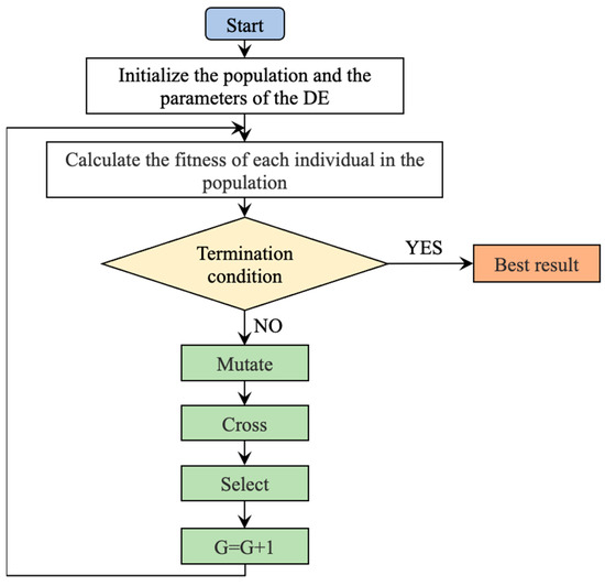
The principle of the DE algorithm is shown in Figure 4.

The DE algorithm starts searching from a group, that is, multiple points instead of the same point [45]. This is the main reason why it can find the overall optimal solution with a greater probability. The evolution criterion of the DE algorithm is based on fitness information [46] with the help of other auxiliary information. It has inherent parallelism, which is suitable for large-scale parallel distributed processing [47]. The DE parameter settings are shown in

Table 1. Parameters optimized by the DE algorithm.

Parameter	Symbol	Value
Dimensions of the objective function	n_dim	9
Maximum number of iterations	max_iter	200
Population size	size_pop	30
Mutation probability	prob_mut	0.8
Crossover probability	Crossp	0.7

.

The DBN input layer has nine channels. They are the theoretical position coordinates of the robot and the angles of the corresponding six joints $\left(\mathit{x},\mathit{y},\mathit{z},{\mathit{\theta }}_1,{\mathit{\theta }}_2,{\mathit{\theta }}_3,{\mathit{\theta }}_4,{\mathit{\theta }}_5,{\mathit{\theta }}_6\right)$. The output layer of DBN is three channels, which are the position error $\left({\mathit{e}}_x,{\mathit{e}}_y,{\mathit{e}}_z\right)$ of the robot.

The maximum number of hidden layers of DBN nodes is set to four layers. The range of nodes in the hidden layer is (10, 101). The initial learning rate is 0.01. The momentum factor is 0.8. The activation function is Sigmoid, and the MSE is used as the loss function. The hyperparameters that need to be optimized are the number of hidden layers of the DBN, number of hidden-layer nodes, learning rate, momentum factor, RBM iterations, and DBN fine-tuning iterations. The hyperparameters are shown in

Table 2. Parameters and optimization range of the DBN.

Parameter	Symbol	Range
Number of hidden layers of DBN	nlayer	(1, 4)
Number of nodes in DBN hidden layer 1	hidden_units [1]	(10, 101)
Number of nodes in DBN hidden layer 2	hidden_units [2]	(10, 101)
Number of nodes in DBN hidden layer 3	hidden_units [3]	(10, 101)
Number of nodes in DBN hidden layer 4	hidden_units [4]	(10, 101)
Learning rate of DBN	learning_rate	(0.01, 1)
Momentum factor of DBN	momentum	(0.8, 1)
Iterations of RBM	epoch_pretrain	(1, 100)
Fine-tuning iterations of DBN	epoch_finetune	(1, 200)

.

3. Supervised Predictive Optimization Based on Evidence Theory

The evidence theory is used as a supervised approach for assessing the uncertainty of DBN predictions. In order to assess the credibility of the DBN prediction, the uncertainty of the DBN prediction is evaluated [48]. This approach is taken to prevent the model from making mistakes due to overconfident performance and to improve the reliability of the prediction system. Evidence theory is a mathematical reasoning method with the characteristic of clearly expressing uncertainty. At present, in most cases, the basic probability assignment function is obtained by referring to expert experience and knowledge [49,50].

3.1. Evidence Theory

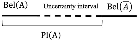
Evidence theory, also known as the Dempster–Shafer (DS) theory [51], is an uncertain reasoning theory widely used in the fields of information fusion and uncertain reasoning. The evidence theory can fuse evidence with comprehensible composite rules without prior probability. It can effectively deal with cognitive uncertainty in various engineering fields [52]. It can describe the corresponding fluctuation range of the system output through two boundary values: the belief function and the likelihood function. The fusion framework of the evidence theory usually consists of three parts: representation of evidence, fusion of evidence, and decision making of evidence [53].

The evidence theory is built on a framework of identification (FD) [54], usually represented by a nonempty set $\Theta$, $\Theta =\left\{{\mathit{\theta }}_1,{\mathit{\theta }}_2,\cdots ,{\mathit{\theta }}_n\right\}$. $\mathit{\theta }$ represents independent elements of a collection. The identification framework has $2^n$ subsets in total. Each subset $\mathit{A}$ corresponds to a possible outcome of a proposition, that is, the proposition $\left\{{\mathit{\theta }}_i,{\mathit{\theta }}_j\right\}$ indicates that at least one of the two basic events is true. The confidence interval is usually used to describe events due to the lack of subjective knowledge.

The confidence interval is a closed interval composed of a belief function $\left(\mathit{B}\mathit{e}\mathit{l}\right)$ and a likelihood function $\left(\mathit{P}\mathit{l}\right)$, which is used to indicate the degree of support for event $\mathit{\theta }$ [55]. $\mathit{B}\mathit{e}\mathit{l}\left(\mathit{A}\right)$ is the sum of the basic probability distributions of all subsets of $\mathit{A}$, which indicates the degree of trust in $\mathit{A}$. It is expressed as:

$$\{\begin{array}{l}\mathit{B}\mathit{e}\mathit{l}\left(\mathit{A}\right)={\displaystyle \sum _{\mathit{B}\subseteq \mathit{A}}\mathit{m}\left(\mathit{B}\right)}\hfill \\ \mathit{A}\subseteq \Theta \hfill \end{array}$$

(14)

$\mathit{P}\mathit{l}\left(\mathit{A}\right)$ is the sum of the basic probability assignments of all subsets intersecting with $\mathit{A}$. It indicates the degree of non-denial to $\mathit{A}$. It is expressed as:

$$\{\begin{array}{l}\mathit{P}\mathit{l}\left(\mathit{A}\right)={\displaystyle \sum _{\mathit{B}\cap \mathit{A}\ne \varnothing }\mathit{m}\left(\mathit{B}\right)}\hfill \\ \mathit{A}\subseteq \Theta \hfill \end{array}$$

(15)

Let the finite nonempty set $\Theta =\left\{{\mathit{\theta }}_1,{\mathit{\theta }}_2,\cdots ,{\mathit{\theta }}_n\right\}$ be the identification framework, and the function $\mathit{m}:2^n\to \left[0,1\right]$ be the basic probability assignment function on the identification framework $\Theta$. In this study, $\mathit{B}\mathit{e}\mathit{l}$ and $\mathit{P}\mathit{l}$ represent the upper and lower bounds of the reliability of the positioning accuracy of industrial robots. For the hypothetical conclusion $\mathit{A}$ in the identification framework, $\mathit{B}\mathit{e}\mathit{l}\left(\mathit{A}\right)$ and $\mathit{P}\mathit{l}\left(\mathit{A}\right)$ form a confidence interval denoted $\mathit{B}\mathit{e}\mathit{l}\left(\mathit{A}\right)$, $\mathit{P}\mathit{l}\left(\mathit{A}\right)$.

This represents a propositional uncertainty, where the probability of the occurrence of proposition $\mathit{A}$ lies somewhere between $\mathit{B}\mathit{e}\mathit{l}$ and $\mathit{P}\mathit{l}$ bounds. It is shown in Figure 5.

3.2. Optimization of Position Error Based on Evidence Theory

This study evaluates the uncertainty of DBN prediction using the evidence theory. It combines the evidence theory with the DBN model and achieves the fusion of evidence through the basic probability assignment function and the Dempster combination rule. The evidence theory does not rely on prior information [56] and is relatively more suitable for situations where it is inconvenient to obtain prior probability and conditional probability [57]. In the DBN prediction task, n feature vectors of the input sample are represented as $\mathit{\phi }\left(\mathit{x}\right)=\left({\mathit{\phi }}_1\left(\mathit{x}\right),{\mathit{\phi }}_2\left(\mathit{x}\right),\cdots ,{\mathit{\phi }}_n\left(\mathit{x}\right)\right)$. The identification frame $\Theta =\left\{{\mathit{\theta }}_1,{\mathit{\theta }}_2,\cdots ,{\mathit{\theta }}_k\right\}$ can be regarded as evidence corresponding to a subset in the identification frame. For each category ${\mathit{\theta }}_k$, evidence ${\mathit{\phi }}_j\left(x\right)$ can be considered to support either $\left\{{\mathit{\theta }}_k\right\}$ or $\overline{\left\{{\mathit{\theta }}_{\mathit{k}}\right\}}$, and the specific support depends on the weight coefficient of the evidence ${\mathit{\phi }}_j\left(\mathit{x}\right)$:

$$\mathit{\omega }=\mathit{\beta }{\mathit{\phi }}_{\mathit{j}}\left(\mathit{x}\right)+\mathit{\alpha }$$

(16)

where $\mathit{\beta }$ and $\mathit{\alpha }$ are two weight parameters.

Assume that the evidence weights of $\left\{{\mathit{\theta }}_{\mathit{k}}\right\}$ and $\overline{\left\{{\mathit{\theta }}_{\mathit{k}}\right\}}$ are the positive and negative parts of $\mathit{\omega }$, respectively. For each ${\mathit{\phi }}_j\left(\mathit{x}\right)$ and each category ${\mathit{\theta }}_k$, two basic probability assignment functions exist:

$${\mathit{m}}^{+}={\left\{{\mathit{\theta }}_{\mathit{k}}\right\}}^{{\mathit{\omega }}^{+}}$$

(17)

$${\mathit{m}}^{-}={\left\{{\mathit{\theta }}_{\mathit{k}}\right\}}^{{\mathit{\omega }}^{-}}$$

(18)

where ${\mathit{m}}^{+}$ represents ${\mathit{\phi }}_j\left(\mathit{x}\right)$ support for $\left\{{\mathit{\theta }}_{\mathit{k}}\right\}$, and ${\mathit{m}}^{-}$ represents ${\mathit{\phi }}_j\left(\mathit{x}\right)$ support for $\overline{\left\{{\mathsf{\theta }}_{\mathit{k}}\right\}}$.

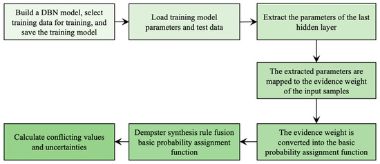
The process of quantitative evaluation method for the uncertainty of DBN prediction is mainly divided into two stages. The first stage is the construction stage of the evidence classifier. The appropriate DBN model is built according to the needs, and the training samples are used to train the model to ensure that the model can meet the requirements of high classification accuracy. The model is saved. The model parameters are loaded. The parameters of the last hidden layer of the model are extracted. The extracted parameters are converted into the basic probability assignment function. The Dempster synthesis rule is used to combine and output the final basic probability assignment function.

The second stage is the uncertainty modeling of DBN prediction. The basic probability assignment function is used as the decision index to predict the classification results. At the same time, the basic probability assignment function is further calculated to obtain the conflict value and uncertainty. The uncertainty of DBN prediction is quantitatively evaluated using the uncertainty evaluation module. The uncertainty evaluation method for DBN prediction is shown in Figure 6.

The evaluation method proposed earlier is based on the evidence classifier. The evidence classifier is modeled by extracting the parameters of the hidden layer of the trained DBN model. During the modeling process, the modification of the training loss function and the retraining of the DBN model are not required. Such characteristics mean that the evaluation method can be applied to any pre-trained DBN model and has strong scalability in the application of the DBN model.

4. Experiments

4.1. Experimental Setup and Data Collection

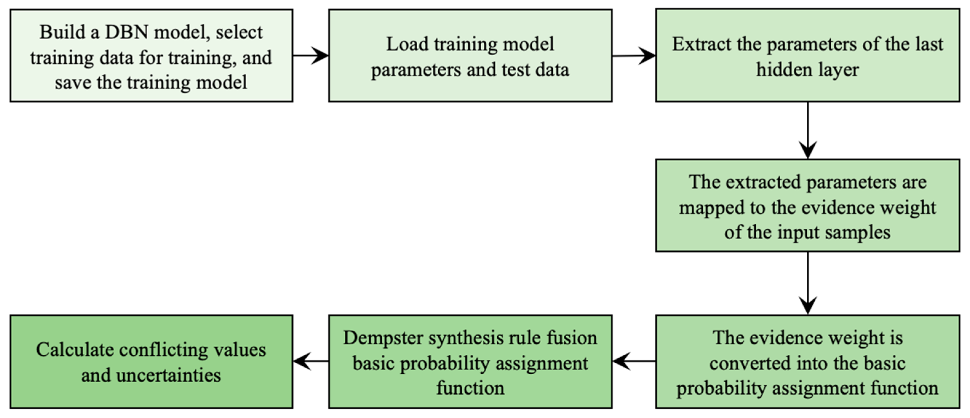
The experimental platform for compensating absolute positioning accuracy compensation of industrial robots is shown in Figure 7. The industrial robot used for precision compensation is KUKA’s KR6_R700 sixx_CR. It has a load capacity of 6 kg and a working range of 700 mm radius. The volume of the working space is 1.36 m³, the position repeatability is ±0.03 mm, and the absolute positioning accuracy is ±0.6 mm. A Leica AT901-B laser tracker is used to measure the position error and the error is ±15 μm + 6 μm/m. The error of the laser tracker increases with the increase in distance.

AT901-B uses an angle encoder to measure the angle and an absolute interferometer to measure the distance. The absolute interferometer in the AT901 integrates a helium-neon laser interferometer and an absolute range finder. The two lasers can work independently. The laser beam emitted by the laser is directed to the target through the universal mirror. The interferometer laser beam also serves as the collimation axis for the tracker. The reflected laser light is measured using the tracker’s built-in dual-axis position detector. The pulse generated by the position detector is processed by the processor of the tracker. The output is then fed back to the servo motor, which drives the motor to track the target mirror of the tracker in real time. Finally, the tracking distance measurement is realized, which is used to measure the actual pose of the end effector of the industrial robot.

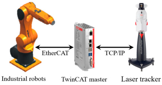
The control and communication diagram of the error compensation platform is shown in Figure 8. The computer is used as the TwinCAT master, that is, the primary controller of the control system. The TwinCAT master uses industrial Ethernet EtherCAT to communicate with industrial robots. The laser tracker communicates with the TwinCAT master via Ethernet (TCP/IP protocol).

In this study, an off-line compensation method [58] is adopted, which uses a laser tracker to obtain the actual position of the manipulator. The DBN based on the DE algorithm is employed to perform the error compensation function.

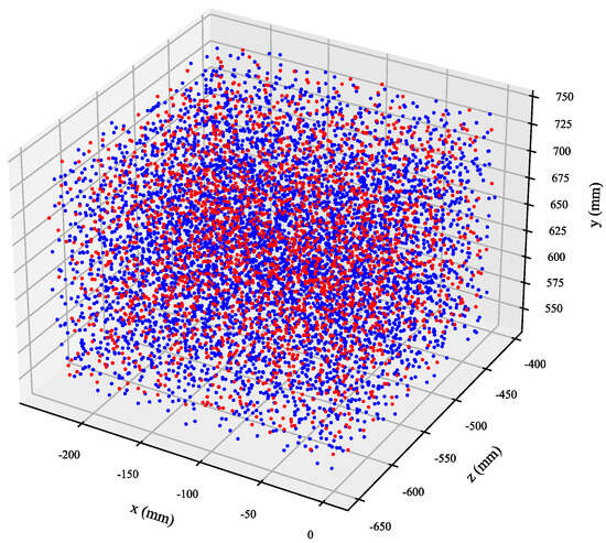
Assuming that the measurement requirements of the laser tracker are met, the target ball of the fixed tooling of the industrial robot is installed in the 240 mm × 240 mm × 200 mm working space, and about 8000 sets of data are measured. For the universality and randomness of the experimental data, the random number module $drand$ is used in TwinCAT3 to randomly generate specific sampling data within a predetermined sampling space. In order to obtain the real position of the robot and the laser tracker in steady state, each sampling is divided into three steps. First, the robot arrives at the sampling point and remains there for 2000 ms. Then, the laser tracker records the data for 1000 ms. Finally, the devices are delayed for another 1000 ms in order to reset them. The theoretical position coordinates and joint angles of the robot are the input of the model. The absolute position error of the robot end constitutes the output of the model.

The data set is divided into the training set and the test set in a ratio of 0.3. The 8000 sets of collected data are divided into 5600 sets of training data and 2400 sets of test data. As shown in Figure 9, the blue dots represent the training set and the red dots represent the test set.

4.2. Model Training and Result Analysis

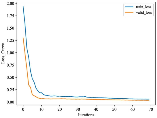
According to the setting in Section 2.2, the input layer of DBN has nine channels, which are the theoretical position coordinates and joint angles of the robot $\left(\mathit{x},\mathit{y},\mathit{z},{\mathit{\theta }}_1,{\mathit{\theta }}_2,{\mathit{\theta }}_3,{\mathit{\theta }}_4,{\mathit{\theta }}_5,{\mathit{\theta }}_6\right)$. The output layer of DBN has three channels, which are the position error $\left({\mathit{e}}_x,{\mathit{e}}_y,{\mathit{e}}_z\right)$ of the robot. Figure 10 shows the loss function decline curve when the DBN is trained alone.

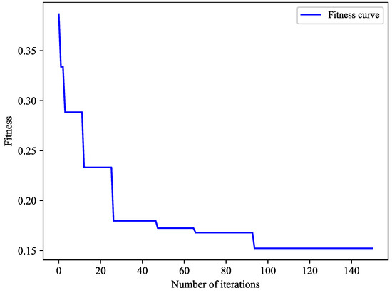
The DE algorithm is utilized to determine the number of hidden layers of the DBN, number of nodes in the hidden layer, learning rate, momentum factor, number of iterations of RBM, and number of iterations of DBN fine-tuning. Figure 11 shows the fitness decline curve of the DE-optimized DBN, which is reduced by 60.7% from 0.387 to 0.152. After 150 iterations of training, the optimal fitness iteration number can be found at the end of the 92nd iteration, and the optimal parameters of the DBN can be output.

The DE algorithm is utilized to determine the number of hidden layers of the DBN, number of hidden-layer nodes, learning rate, momentum factor, number of iterations of RBM, and number of iterations of DBN fine-tuning. The fitness of each particle is calculated according to the fitness calculation conditions. When the training error reaches the allowable value or the number of iterations reaches the maximum value, the DE algorithm iteration terminates.

Finally, the DBN hyperparameters determined according to the DE algorithm are shown in

Table 3. Optimal parameters of DBN.

Parameter	Symbol	Optimal Value
Number of hidden layers of DBN	nlayer	4
Number of nodes in DBN hidden layer 1	hidden_units [1]	7
Number of nodes in DBN hidden layer 2	hidden_units [2]	56
Number of nodes in DBN hidden layer 3	hidden_units [3]	62
Number of nodes in DBN hidden layer 4	hidden_units [4]	56
Learning rate of DBN	learning_rate	0.9360
Momentum factor of DBN	momentum	0.9618
Iterations of RBM	epoch_pretrain	100
Fine-tuning iterations of DBN	epoch_finetune	70

.

Supervised learning in machine learning essentially yields a series of training samples and establishes a mapping relationship so that the fitting result is as close as possible to the real output. The loss function is an important indicator for analyzing the quality of the training results. In this paper, the DBN is analyzed using five indicators: MSE, root mean square error (RMSE), mean absolute percentage error (MAPE), mean absolute error (MAE), and R². These five indicators are expressed as follows:

$$\mathrm{MSE}=\frac{1}{n}{\displaystyle \sum _{i=1}^n{\left(y_i-{\widehat{y}}_i\right)}^2}$$

(19)

$$\mathrm{RMSE}=\sqrt{\frac{1}{n}{\displaystyle \sum _{i=1}^n{\left(y_i-{\widehat{y}}_i\right)}^2}}=\sqrt{\mathrm{MSE}}$$

(20)

$$\mathrm{MAPE}=\frac{1}{n}{\displaystyle \sum _{i=1}^n\frac{\left|y_i-{\widehat{y}}_i\right|}{y_i}}$$

(21)

$$\mathrm{MAE}=\frac{1}{n}{\displaystyle \sum _{i=1}^n\left|y_i-{\widehat{y}}_i\right|}$$

(22)

$${\mathrm{R}}^2=1-\frac{{\displaystyle \sum _{i=1}^n{\left(y_i-{\widehat{y}}_i\right)}^2}}{{\displaystyle \sum _{i=1}^n{\left(y_i-{\overline{y}}_i\right)}^2}}=1-\frac{\mathrm{RMSE}}{\mathrm{Var}}$$

(23)

where $y_i$ represents the true value of the data set. ${\widehat{y}}_i$ represents the predicted value of the data set. ${\overline{y}}_i$ represents the average value of the predicted value of the data set. $n$ represents the number of data sets. Var represents the data variance.

MSE is the mean of the sum of squares of the corresponding point errors between the predicted data and the original data. RMSE is the square root of MSE, also known as the fitting standard deviation of the regression system. MAPE is often used to measure the accuracy of predictions. However, when the real data are equal to zero, the denominator becomes zero and the formula is not available. The situation where the true value is zero does not appear in this study. The MAE refers to the average value of the absolute value of the deviation of each measurement value, which accurately reflects the size of the actual prediction error. The closer the four indicators approach 0, the closer the predicted value will be to the real value, indicating a better prediction effect.

R² represents the coefficient of determination of the model. The best score is 1, indicating that the model perfectly predicts the real value. It may also be negative because the model can be arbitrarily worse, that is, no mapping-fitting relationship exists between the predicted data and the real data.

Table 4. MSE, RMSE, MAPE, MAE, and R² values.

	$\mathit{x}$	$\mathit{y}$	$\mathit{z}$
MSE	0.0104	0.0017	0.0003
RMSE	0.1021	0.0412	0.0194
MAPE	0.1021	0.0412	0.0193
MAE	0.0824	0.0284	0.0900
R2	0.8701	0.9038	0.9582

shows the calculated MSE, RMSE, MAPE, MAR, and R² from the DBN model.

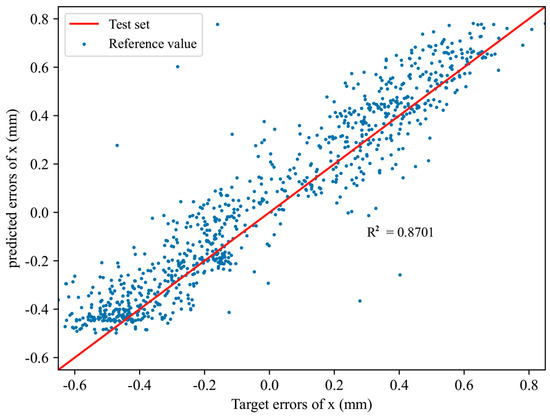
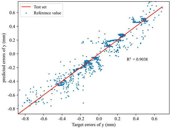
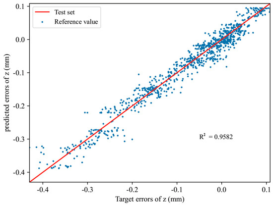
The MSE, RMSE, MAPE, and MAE of the position error prediction value of the robot end effector are all found to be close to 0 using the proposed position error prediction model for industrial robots. The coefficient of determination (R²) of the predicted value of the position error is shown in Figure 12, Figure 13 and Figure 14. The figures show that the predicted value (blue dot) is closely distributed around the real value (red line). In addition, R² is close to 1, indicating the correlation between the predicted value and the actual value. The higher the value, the higher the fitting accuracy. Therefore, the proposed machine learning model has good adaptability and robustness in the prediction of industrial robot position errors.

The R² of the robot end precision compensation error is around 0.87–0.95, and the overall effect is good. As the DBN is trained and iterated in three dimensions, the characteristics of the three dimensions interact and couple with each other. It is also disturbed by nonlinear factors such as the accuracy of data acquisition and environmental conditions, which makes some differences in the effect of robot end accuracy error compensation.

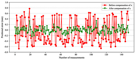
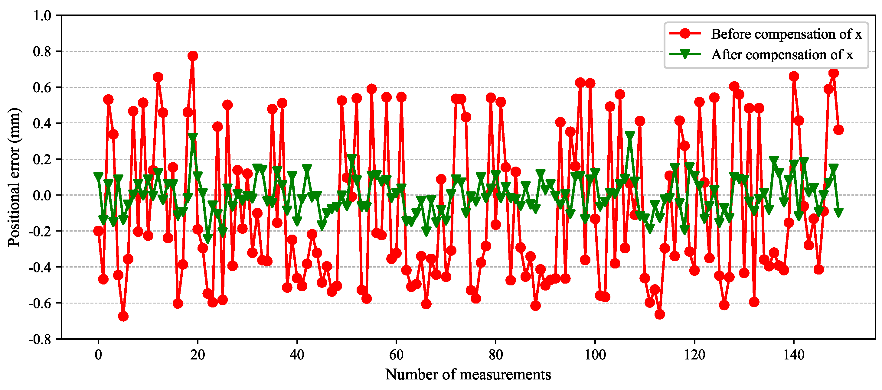
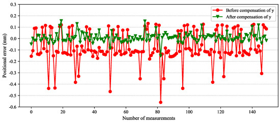
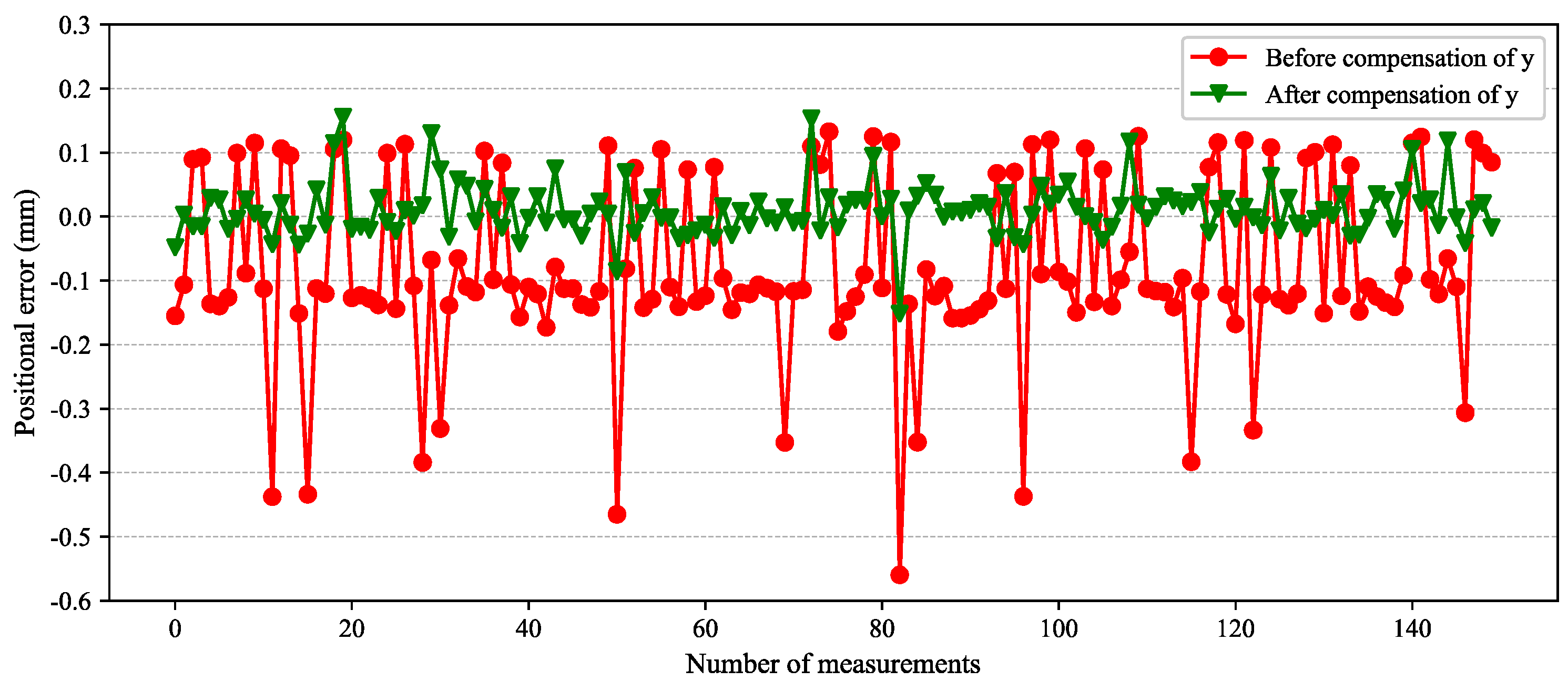
A total of 50 random verification points were selected in the robot motion space with a measurement space of 240 × 240 × 200 mm³. These are presented to verify the effectiveness and improvement effect of the DBN optimization based on the DE algorithm. The distribution of position errors before and after compensation in the $x$, $y$, and $z$ directions are shown in Figure 15, Figure 16 and Figure 17, respectively. The compensation results revealed the following. Before compensation, the errors in the $x$ direction are basically evenly distributed above and below 0. The errors in the $y$ direction are also distributed around 0, but are more negative. The errors in the $z$ direction are basically negative. The error compensation technology proposed in this study is used to optimize the DBN with the DE algorithm. The errors in the three directions are basically distributed around 0 and fluctuate around ±0.2 mm, ±0.1 mm, and ±0.5 mm. The range of fluctuations is extremely small, indicating that the accuracy after compensation has high stability and that the accuracy of robot operation can be improved.

Table 5. Statistical results of the positional errors.

		Error Range	Confidence	Percent Improvement
$x$ error (mm)	Before	[−0.674, 0.773]	[−0.500, 0.345]	65.56%
	After	[−0.130, 0.368]	[−0.017, 0.017]
$y$ error (mm)	Before	[0.133, −0.559]	[−0.225, 0.063]	55.22%
	After	[0.108, −0.201]	[−0.047, 0.031]
$z$ error (mm)	Before	[0.003, −0.162]	[−0.115, −0.026]	49.12%
	After	[0.029, −0.054]	[−0.021, 0.009]

shows the static statistical analysis results before and after the robot end position error compensation. The $x$, $y$, and $z$ directions are improved by 65.56%, 55.22%, and 49.12%, respectively.

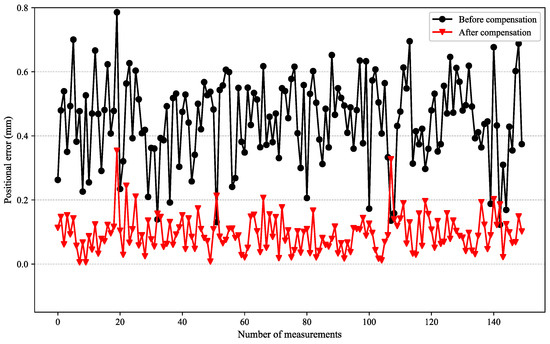
The experimental platform for data acquisition and verification of the robot is the light industrial robot KR6_R700 sixx_CR. The error range is much smaller compared with that of the traditional heavy industrial robot. Hence, using the DBN for feature extraction, model training, and optimization is difficult. The network is optimized and combined with the evidence theory, and the position error mapping model of industrial robots is established. The comprehensive analysis of the compensation effect of the robot end accuracy in three directions is shown in Figure 18.

The method used in this study is compared with previous methods to verify the test results [25,27]. The results are shown in

Table 6. Comparison of data compensation on the results of previous models.

Error (mm)	Max	Min	Average
Uncompensated	1.529	0.124	0.754
GA-DNN	0.965	0.017	0.284
PSO-DNN	0.519	0.172	0.333
GPSO-DNN	0.364	0.097	0.249
PSO-DBN	0.244	Null	0.110
Uncompensated	0.701	0.139	0.469
DE-DBN	0.255	0.006	0.083

. After off-line compensation, the minimum value is reduced from 0.097 mm to 0.006 mm. The average value is reduced from 0.110 mm to 0.083 mm. Therefore, the proposed DE-DBN method was successful in improving the minimum and average values after the end error compensation of the robot.

5. Conclusions

Based on deep belief networks using an off-line compensation method, a compensation algorithm for the absolute positioning accuracy of industrial robots is proposed. It predicts and compensates for the absolute positioning error of industrial robots based on the DBN and DE algorithm. The number of hidden layers, hidden-layer nodes, learning rate, momentum factors, RBM iterations, and DBN fine-tuning iterations are optimized. The position error model of industrial robots is established. Combined with the off-line feedback compensation method, the proposed method is verified experimentally using the KR6_R700 sixx_CR industrial robot and the AT901-B laser tracker.

After compensation, the absolute positioning error of the robot end is reduced by 82.14%, from 0.469 mm to 0.084 mm. The absolute positioning accuracy of the industrial robot is improved. This indicates the proposed approach is advantageous for performing more precise operation tasks. The results of this paper can be used to improve the absolute positioning accuracy of industrial robots, which is of great help in improving the motion accuracy and force control performance of robots.

Considerations of the off-line compensation method include an experimental environment free of vibration, the allowable operating temperature of the robot, and the higher accuracy of the laser tracker. Future work can further consider industrial robot load, motion speed, acceleration, ambient temperature, or other factors that affect the absolute positioning accuracy of the robot. Deep learning can be integrated into the robot’s motion control system. The training model can be deployed in the control algorithm. Realizing the intelligent prediction and real-time compensation of robot errors is a direction of great research value.

References

- Mubarak, M.F.; Petraite, M. Industry 4.0 Technologies, Digital Trust and Technological Orientation: What Matters in Open Innovation? Technol. Forecast Soc. Chang. 2020, 161, 120332. [Google Scholar] [CrossRef]
- Papakostas, N.; Constantinescu, C.; Mourtzis, D. Novel Industry 4.0 Technologies and Applications. Appl. Sci. 2020, 10, 6498. [Google Scholar] [CrossRef]
- Jaskó, S.; Skrop, A.; Holczinger, T.; Chován, T.; Abonyi, J. Development of Manufacturing Execution Systems in Accordance with Industry 4.0 Requirements: A Review of Standard- and Ontology-Based Methodologies and Tools. Comput. Ind. 2020, 123, 103300. [Google Scholar] [CrossRef]
- Rosin, F.; Forget, P.; Lamouri, S.; Pellerin, R. Impacts of Industry 4.0 Technologies on Lean Principles. Int. J. Prod. Res. 2019, 58, 1644–1661. [Google Scholar] [CrossRef]
- Moosavi, J.; Bakhshi, J.; Martek, I. The Application of Industry 4.0 Technologies in Pandemic Management: Literature Review and Case Study. Healthc. Anal. 2021, 1, 100008. [Google Scholar] [CrossRef]
- Klerkx, L.; Rose, D. Dealing with the Game-Changing Technologies of Agriculture 4.0: How Do We Manage Diversity and Responsibility in Food System Transition Pathways? Glob. Food Sec. 2020, 24, 100347. [Google Scholar] [CrossRef]
- Javaid, M.; Haleem, A.; Khan, I.H.; Suman, R. Understanding the Potential Applications of Artificial Intelligence in Agriculture Sector. Adv. Agrochem. 2023, 2, 15–30. [Google Scholar] [CrossRef]
- Strong, R.; Wynn, J.T.; Lindner, J.R.; Palmer, K. Evaluating Brazilian Agriculturalists’ IoT Smart Agriculture Adoption Barriers: Understanding Stakeholder Salience Prior to Launching an Innovation. Sensors 2022, 22, 6833. [Google Scholar] [CrossRef]
- Ronaghi, M.; Ronaghi, M.H. Investigating the Impact of Economic, Political, and Social Factors on Augmented Reality Technology Acceptance in Agriculture (Livestock Farming) Sector in a Developing Country. Technol. Soc. 2021, 67, 101739. [Google Scholar] [CrossRef]
- Osinga, S.A.; Paudel, D.; Mouzakitis, S.A.; Athanasiadis, I.N. Big Data in Agriculture: Between Opportunity and Solution. Agric. Syst. 2022, 195, 103298. [Google Scholar] [CrossRef]
- Ahn, J.; Briers, G.; Baker, M.; Price, E.; Sohoulande Djebou, D.C.; Strong, R.; Piña, M.; Kibriya, S. Food Security and Agricultural Challenges in West-African Rural Communities: A Machine Learning Analysis. Int. J. Food Prop. 2022, 25, 827–844. [Google Scholar] [CrossRef]
- Zheng, T.; Ardolino, M.; Bacchetti, A.; Perona, M. The Applications of Industry 4.0 Technologies in Manufacturing Context: A Systematic Literature Review. Int. J. Prod. Res. 2021, 59, 1922–1954. [Google Scholar] [CrossRef]
- Frank, A.G.; Dalenogare, L.S.; Ayala, N.F. Industry 4.0 Technologies: Implementation Patterns in Manufacturing Companies. Int. J. Prod. Econ. 2019, 210, 15–26. [Google Scholar] [CrossRef]
- Javaid, M.; Haleem, A.; Singh, R.P.; Suman, R. Substantial Capabilities of Robotics in Enhancing Industry 4.0 Implementation. Cogn. Robot. 2021, 1, 58–75. [Google Scholar] [CrossRef]
- Zhang, T.; Yu, Y.; Yang, L.X.; Xiao, M.; Chen, S.Y. Robot Grinding System Trajectory Compensation Based on Co-Kriging Method and Constant-Force Control Based on Adaptive Iterative Algorithm. Int. J. Precis. Eng. Manuf. 2020, 21, 1637–1651. [Google Scholar] [CrossRef]
- Wang, W.; Tian, W.; Liao, W.; Li, B. Pose Accuracy Compensation of Mobile Industry Robot with Binocular Vision Measurement and Deep Belief Network. Optik 2021, 238, 166716. [Google Scholar] [CrossRef]
- Qi, J.; Chen, B.; Zhang, D. Compensation for Absolute Positioning Error of Industrial Robot Considering the Optimized Measurement Space. Int. J. Adv. Robot Syst. 2020, 17. [Google Scholar] [CrossRef]
- Kong, L.B.; Yu, Y. Precision Measurement and Compensation of Kinematic Errors for Industrial Robots Using Artifact and Machine Learning. Adv. Manuf. 2022, 10, 397–410. [Google Scholar] [CrossRef]
- Cao, C.T.; Do, V.P.; Lee, B.R. A Novel Indirect Calibration Approach for Robot Positioning Error Compensation Based on Neural Network and Hand-Eye Vision. Appl. Sci. 2019, 9, 1940. [Google Scholar] [CrossRef]
- Chen, D.; Yuan, P.; Wang, T.; Cai, Y.; Xue, L. A Compensation Method for Enhancing Aviation Drilling Robot Accuracy Based on Co-Kriging. Int. J. Precis. Eng. Manuf. 2018, 19, 1133–1142. [Google Scholar] [CrossRef]
- Chen, D.; Yuan, P.; Wang, T.; Ying, C.; Tang, H. A Compensation Method Based on Error Similarity and Error Correlation to Enhance the Position Accuracy of an Aviation Drilling Robot. Meas. Sci. Technol. 2018, 29, 085011. [Google Scholar] [CrossRef]
- Shen, N.Y.; Guo, Z.M.; Li, J.; Tong, L.; Zhu, K. A Practical Method of Improving Hole Position Accuracy in the Robotic Drilling Process. Int. J. Adv. Manuf. Technol. 2018, 96, 2973–2987. [Google Scholar] [CrossRef]
- Chen, D.; Wang, T.; Yuan, P.; Sun, N.; Tang, H. A Positional Error Compensation Method for Industrial Robots Combining Error Similarity and Radial Basis Function Neural Network. Meas. Sci. Technol. 2019, 30, 125010. [Google Scholar] [CrossRef]
- Wang, L.; Tang, Z.; Zhang, P.; Liu, X.; Wang, D.; Li, X. Double Extended Sliding Mode Observer-Based Synchronous Estimation of Total Inertia and Load Torque for PMSM-Driven Spindle-Tool Systems. IEEE Trans. Ind. Inf. 2022, 19, 8496–8507. [Google Scholar] [CrossRef]
- Fu, S.; Li, Y.; Zhang, M.; Hu, J.; Hua, F.; Tian, W. Robot Positioning Error Compensation Method Based on Deep Neural Network. J. Phys. Conf. Ser. 2020, 1487, 012045. [Google Scholar] [CrossRef]
- LI, B.; TIAN, W.; ZHANG, C.; HUA, F.; CUI, G.; LI, Y. Positioning Error Compensation of an Industrial Robot Using Neural Networks and Experimental Study. Chin. J. Aeronaut. 2022, 35, 346–360. [Google Scholar] [CrossRef]
- Wang, W.; Tian, W.; Liao, W.; Li, B.; Hu, J. Error Compensation of Industrial Robot Based on Deep Belief Network and Error Similarity. Robot Comput. Integr. Manuf. 2022, 73, 102220. [Google Scholar] [CrossRef]
- Qi, J.; Chen, B.; Zhang, D. A Calibration Method for Enhancing Robot Accuracy Through Integration of Kinematic Model and Spatial Interpolation Algorithm. J. Mech. Robot 2021, 13, 061013. [Google Scholar] [CrossRef]
- Adel, M.; Khader, M.M.; Algelany, S. High-Dimensional Chaotic Lorenz System: Numerical Treatment Using Changhee Polynomials of the Appell Type. Fractal. Fract. 2023, 7, 398. [Google Scholar] [CrossRef]
- Adel, M.; Khader, M.M.; Assiri, T.A.; Kallel, W. Numerical Simulation for COVID-19 Model Using a Multidomain Spectral Relaxation Technique. Symmetry 2023, 15, 931. [Google Scholar] [CrossRef]
- Khader, M.M.; Inc, M.; Adel, M.; Akinlar, M.A. Numerical Solutions to the Fractional-Order Wave Equation. Int. J. Mod. Phys. C 2023, 34, 2350067. [Google Scholar] [CrossRef]
- Adel, M.; Srivastava, H.M.; Khader, M.M. Implementation of an Accurate Method for the Analysis and Simulation of Electrical R-L Circuits. Math. Methods Appl. Sci. 2023, 46, 8362–8371. [Google Scholar] [CrossRef]
- Adel, M.; Khader, M.M.; Ahmad, H.; Assiri, T.A.; Adel, M.; Khader, M.M.; Ahmad, H.; Assiri, T.A. Approximate Analytical Solutions for the Blood Ethanol Concentration System and Predator-Prey Equations by Using Variational Iteration Method. AIMS Math. 2023, 8, 19083–19096. [Google Scholar] [CrossRef]
- Ibrahim, Y.F.; Abd El-Bar, S.E.; Khader, M.M.; Adel, M. Studying and Simulating the Fractional COVID-19 Model Using an Efficient Spectral Collocation Approach. Fractal. Fract. 2023, 7, 307. [Google Scholar] [CrossRef]
- Min, K.; Ni, F.; Chen, Z.; Liu, H.; Lee, C.-H. A Robot Positional Error Compensation Method Based on Improved Kriging Interpolation and Kronecker Products. IEEE Trans. Ind. Electron. 2023, 1–10. [Google Scholar] [CrossRef]
- Zhou, J.; Zheng, L.; Fan, W.; Zhang, X.; Cao, Y. Adaptive Hierarchical Positioning Error Compensation for Long-Term Service of Industrial Robots Based on Incremental Learning with Fixed-Length Memory Window and Incremental Model Reconstruction. Robot Comput. Integr. Manuf. 2023, 84, 102590. [Google Scholar] [CrossRef]
- Li, R.; Ding, N.; Zhao, Y.; Liu, H. Real-Time Trajectory Position Error Compensation Technology of Industrial Robot. Measurement 2023, 208, 112418. [Google Scholar] [CrossRef]
- Ma, S.; Deng, K.; Lu, Y.; Xu, X. Error Compensation Method of Industrial Robots Considering Non-Kinematic and Weak Rigid Base Errors. Precis. Eng. 2023, 82, 304–315. [Google Scholar] [CrossRef]
- Hinton, G.E.; Osindero, S.; Teh, Y.W. A Fast Learning Algorithm for Deep Belief Nets. Neural Comput. 2006, 18, 1527–1554. [Google Scholar] [CrossRef]
- Gao, S.; Xu, L.; Zhang, Y.; Pei, Z. Rolling Bearing Fault Diagnosis Based on SSA Optimized Self-Adaptive DBN. ISA Trans. 2022, 128, 485–502. [Google Scholar] [CrossRef]
- Wang, Y.; Pan, Z.; Yuan, X.; Yang, C.; Gui, W. A Novel Deep Learning Based Fault Diagnosis Approach for Chemical Process with Extended Deep Belief Network. ISA Trans. 2020, 96, 457–467. [Google Scholar] [CrossRef]
- Liu, J.; Wu, N.; Qiao, Y.; Li, Z. Short-Term Traffic Flow Forecasting Using Ensemble Approach Based on Deep Belief Networks. IEEE Trans. Intell. Transp. Syst. 2022, 23, 404–417. [Google Scholar] [CrossRef]
- Storn, R.; Price, K. Differential Evolution—A Simple and Efficient Heuristic for Global Optimization over Continuous Spaces. J. Glob. Optim. 1997, 11, 341–359. [Google Scholar] [CrossRef]
- Ahmad, M.F.; Isa, N.A.M.; Lim, W.H.; Ang, K.M. Differential Evolution: A Recent Review Based on State-of-the-Art Works. Alex. Eng. J. 2022, 61, 3831–3872. [Google Scholar] [CrossRef]
- Bilal; Pant, M.; Zaheer, H.; Garcia-Hernandez, L.; Abraham, A. Differential Evolution: A Review of More than Two Decades of Research. Eng. Appl. Artif. Intell. 2020, 90, 103479. [Google Scholar] [CrossRef]
- Deng, W.; Shang, S.; Cai, X.; Zhao, H.; Song, Y.; Xu, J. An Improved Differential Evolution Algorithm and Its Application in Optimization Problem. Soft Comput. 2021, 25, 5277–5298. [Google Scholar] [CrossRef]
- Khaparde, A.R.; Alassery, F.; Kumar, A.; Alotaibi, Y.; Khalaf, O.I.; Pillai, S.; Alghamdi, S. Differential Evolution Algorithm with Hierarchical Fair Competition Model. Intell. Autom. Soft Comput. 2022, 33, 1045–1062. [Google Scholar] [CrossRef]
- Fang, Z.; Roy, K.; Mares, J.; Sham, C.W.; Chen, B.; Lim, J.B.P. Deep Learning-Based Axial Capacity Prediction for Cold-Formed Steel Channel Sections Using Deep Belief Network. Structures 2021, 33, 2792–2802. [Google Scholar] [CrossRef]
- Tong, Z.; Xu, P.; Denœux, T. An Evidential Classifier Based on Dempster-Shafer Theory and Deep Learning. Neurocomputing 2021, 450, 275–293. [Google Scholar] [CrossRef]
- Du, Y.W.; Zhong, J.J. Generalized Combination Rule for Evidential Reasoning Approach and Dempster–Shafer Theory of Evidence. Inf. Sci. 2021, 547, 1201–1232. [Google Scholar] [CrossRef]
- Deng, X.; Jiang, W.; Wang, Z. Zero-Sum Polymatrix Games with Link Uncertainty: A Dempster-Shafer Theory Solution. Appl. Math. Comput. 2019, 340, 101–112. [Google Scholar] [CrossRef]
- Gudiyangada Nachappa, T.; Tavakkoli Piralilou, S.; Gholamnia, K.; Ghorbanzadeh, O.; Rahmati, O.; Blaschke, T. Flood Susceptibility Mapping with Machine Learning, Multi-Criteria Decision Analysis and Ensemble Using Dempster Shafer Theory. J. Hydrol. 2020, 590, 125275. [Google Scholar] [CrossRef]
- Pan, Y.; Zhang, L.; Li, Z.W.; Ding, L. Improved Fuzzy Bayesian Network-Based Risk Analysis with Interval-Valued Fuzzy Sets and D–S Evidence Theory. IEEE Trans. Fuzzy Syst. 2020, 28, 2063–2077. [Google Scholar] [CrossRef]
- Xiao, F. Generalization of Dempster–Shafer Theory: A Complex Mass Function. Appl. Intell. 2020, 50, 3266–3275. [Google Scholar] [CrossRef]
- Xiao, F. A New Divergence Measure for Belief Functions in D–S Evidence Theory for Multisensor Data Fusion. Inf. Sci. 2020, 514, 462–483. [Google Scholar] [CrossRef]
- Feng, R.; Xu, X.; Zhou, X.; Wan, J. A Trust Evaluation Algorithm for Wireless Sensor Networks Based on Node Behaviors and D-S Evidence Theory. Sensors 2011, 11, 1345–1360. [Google Scholar] [CrossRef]
- Wang, H.; Deng, X.; Jiang, W.; Geng, J. A New Belief Divergence Measure for Dempster–Shafer Theory Based on Belief and Plausibility Function and Its Application in Multi-Source Data Fusion. Eng. Appl. Artif. Intell. 2021, 97, 104030. [Google Scholar] [CrossRef]
- Slavkovic, N.; Zivanovic, S.; Kokotovic, B.; Dimic, Z.; Milutinovic, M. Simulation of Compensated Tool Path through Virtual Robot Machining Model. J. Braz. Soc. Mech. Sci. Eng. 2020, 42, 374. [Google Scholar] [CrossRef]
Disclaimer/Publisher’s Note: The statements, opinions and data contained in all publications are solely those of the individual author(s) and contributor(s) and not of MDPI and/or the editor(s). MDPI and/or the editor(s) disclaim responsibility for any injury to people or property resulting from any ideas, methods, instructions or products referred to in the content. |
© 2023 by the authors. Licensee MDPI, Basel, Switzerland. This article is an open access article distributed under the terms and conditions of the Creative Commons Attribution (CC BY) license (https://creativecommons.org/licenses/by/4.0/).