Self-Supervised Sound Promotion Method of Sound Localization from Video

Abstract

Compared to traditional unimodal methods, multimodal audio-visual correspondence learning has many advantages in the field of video understanding, but it also faces significant challenges. In order to fully utilize the feature information from both modalities, we needs to ensure accurate alignment of the semantic information from each modality, rather than simply concatenating them together. This requires consideration of how to design fusion networks that can better perform this task. Current algorithms heavily rely on the network’s output results for sound-object localization while neglecting the potential issue of suppressed feature information due to the internal structure of the network. Thus, we propose a sound promotion method (SPM), a self-supervised framework that aims to increase the contribution of voices to produce better performance of the audiovisual learning. We first cluster the audio separately to generate pseudo-labels and then use the clusters to train the backbone of audio. Finally, we explore the impact of our method to several existing approaches on MUSIC datasets and the results prove that our proposed method is able to produce better performance.

1. Introduction

As humans, we not only perceive the world through vision, but also use hearing, tasting, touching, etc. If only an image is provided, the existing algorithm can already meet most of people’s needs, such as object category recognition, action understanding, text translation, etc. But if a video is provided, the original research in the field of single-modal images cannot cover the understanding of the video well, because the video has not only one more time dimension than the image, but also additional sound information, and the image and sound in the video are naturally corresponding, which is the key to join them in our network. Therefore, audio-visual correspondence learning is gradually separated from the original image field and sound field, and combined into a new research direction. Now, with the influx of a large number of researchers, this direction also has many branches, such as speaker separation [1,2,3,4], sound source localization [5,6,7], speech recognition [8,9,10,11], audio-visual retrieval [12,13], etc.

In this paper, we focus on the problem of sound source localization [14] which has recently become one of the mainstream research projects of Audio-Visual Learning (AVL), because we believe that the accuracy of the sound localization reflects the network’s learning of the video. In addition, since there are various unlabeled videos on the Internet, the common starting point of recent work is to learn the position information of the sound in the video in a self-supervised or weakly supervised way. The earlier works feed information from both modalities into the same network [5,6,7,15], like, for example, Arandjelovic et al. [5], who utilized the audiovisual correspondence (AVC) to find the sound localization in 2018. Then, Zhao et al. [16] proposed a mix-and-separate approach to compute the sound of each pixel by an audio synthesizer network, and Senocak et al. [15] fused the information of two modalities by using the attention mechanism which can be applied to supervised or un-supervised learning. In 2019, Hu et al. [17] clustered audio and visual representations within each modality to calculate similarity through contrastive learning. In 2021, Lin et al. [18] extended this method by using an iterative contrastive learning algorithm. Based on this, Chen et al. [19] also proposed a tri-map method to divide a picture into more detailed positive and negative samples, and in 2022, Song et al. [20] discarded negative samples directly to form a negative-free method and propose a predictive coding module (PCM) for feature alignment. At the same time, Senocak et al. [21] used multi-task classification to train the backbone of the audiovisual network.

These methods did localize the sounding object, but they just focus on the image or the image-to-audio relationship and ignore the audio. According to the conclusion in [21], the feature extractor obtained through a classification task is applicable to the research on sound source localization algorithms. Therefore, it can be inferred that the classification accuracy of the two-modal feature extractor followed by a classifier reflects its contribution to the final results. Based on this observation, we connected two classifiers after the image and audio feature extractors, respectively. Through a series of training experiments, it was found that the classification accuracy of the image channel is approximately 65%, while the accuracy of the audio classifier is only about 27%. It turns out that the sound itself was not fully exploited and utilized, which lead to the ambiguity of sound source location. Thus, different from the aforementioned articles, we propose our sound promotion method (SPM) which makes the network pay more attention to the audio and obtains a more precise localization of the sound source. The procedure is as follows: First, since we want to improve the contribution of audio, we cluster audio information features separately. 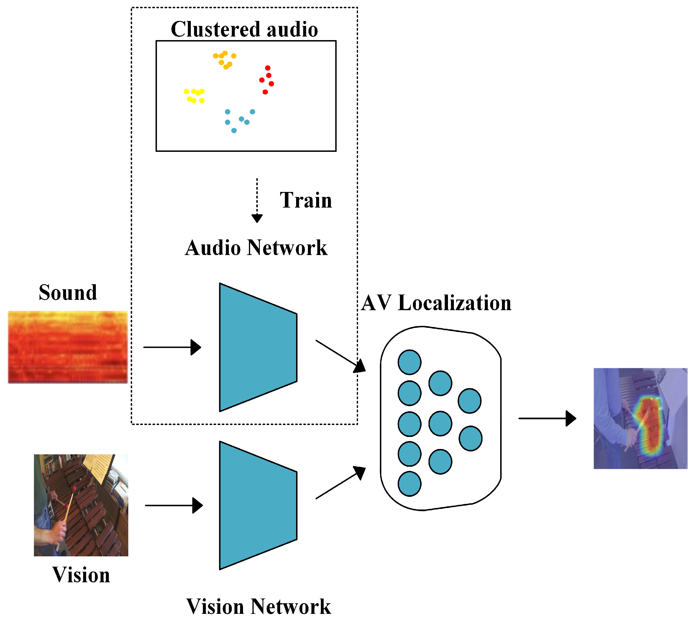Then, we use the pseudo-label of sound to train the backbone of the audio (Figure 1). We freeze this part and train the whole network, because we find that with the network training, the entire network focuses on the image level, which makes the audio contribution decline. Finally, the results indicate that our method greatly improves the accuracy, which proves the effectiveness of our method.

As Figure 1 shows, our method mainly includes three key parts: the audio image feature extraction network, the sound promotion framework and the multi-modal fusion framework (AV localization). The audio and image feature extraction networks are designed using the first five layers of a ResNet-18 model with a residual structure. Considering that the audio input is a mel-log spectrum, i.e., a one-dimensional signal, the number of audio channels is set to one in the first layer of the audio extractor. Meanwhile, for image input, the image frames in the video are randomly selected as input. At the same time, the image feature extraction network is obtained by pre-training on the ImageNet Datasets, while the audio feature extraction network uses the sound promotion method (SPM) proposed in this study which uses sound clustering to generate pseudo-label categories for training, freezing its parameters and then performing transfer learning. Through these two feature extraction networks, high-level semantic information of images and sounds can be obtained. Subsequently, this information is input into the multi-modal fusion framework for settlement. In this framework, by calculating the cosine similarity between the image and the sound, and through a sigmoid function, a mask consistent with the size of the image is generated to obtain the information of the sounding object in the image. Since images and audio come from the same video, there is a natural correspondence between them, so they are used as pseudo-labels to supervise the learning network to achieve the goal of self-supervised learning. In the end, the mask generated by the network is able to accurately localize the location of the sounding object.

Our main contributions of this work are summarized as follows: (1) We mine the contribution of audio and image to the results. (2) We propose a novel sound promotion method (SPM). It clusters the audio separately to generate pseudo-labels and then uses the clusters to train the backbone of audio. (3) We explore the impact of our method on several existing approaches on MUSIC datasets [18] which show that our method can improve the sound source localization.

2. Materials and Methods

The goal of our model is to localize sound sources by increasing the contribution of voice to the whole network. Most of the existing works [17,19,20,22] are all about improvement in the field of image, and they do not consider optimizing audio as one of the modalities to improve network performance.

Different from the aforementioned methods, our method is shown in Figure 1 in the dashed frame and can be explained as follows. Because our method is validated on DSOL [23] as the baseline, we first introduce the model of the baseline, and then introduce our method.

2.1. Audiovisual Model of the Baseline

We obtain visual frames $v_i$ and audio spectrogram $a_j$ from video clips $X=\{v_i,a_j|v_i\in R^{C\times H\times W},a_j\in R^C\}$; H and W are the spatial size. Then, we obtain their visual feature representation $V_i$ and audio feature representation $A_j$ through vision embedding ${\mathit{f}}_v\left(·\right)$ and audio embedding ${\mathit{f}}_a\left(·\right)$.

$$\begin{array}{cc}\hfill & \hfill V_i={\mathit{f}}_v\left(v_i\right),v_i\in R^{C\times H\times W},\hfill \end{array}$$

(1)

$$\begin{array}{cc}\hfill & \hfill A_j={\mathit{f}}_a\left(a_j\right),a_j\in R^C.\hfill \end{array}$$

(2)

Note that it is regarded as a positive sample that the audio and image are from the same video, i.e., $i=j$. Otherwise, when they come from different videos, i.e., $i\ne j$, the value is perceived as a negative sample.

In addition, the cosine similarities are computed in Equation (3) by feeding the vision and audio features, $V_i$ and $A_j$.

$${\left[cosin{e}_{ij}\right]}_{uv}=\frac{〈A_j,{\left[V_i\right]}_{:uv}〉}{∥A_j∥∥{\left[V_i\right]}_{:uv}∥},uv\in \left[h\right]\times \left[w\right].$$

(3)

Then, we use the sigmoid function $\sigma$ to obtain the mask of sounding object $m_{ij}$ as follows:

$$m_{ij}=\sigma \left(\left(cosin{e}_{ij}-ϵ\right)/\tau \right),$$

(4)

where $ϵ$ refers to the thresholding parameter and $\tau$ is the temperature. Hence, we can extract potential object representation $O_i$ which represents the degree of correlation between audio and video,

$$O_i=GAP\left({\mathit{f}}_v\left(v_i\right)\circ m_{ij}\right),$$

(5)

where $GAP$ is the Global Average Pooling operation and ∘ is the Hadamard product.

2.2. Sound Similar Mining

As we have lots of audio information, clustering is the most efficient way for self-supervision. We cluster the audio representation $A_j$ obtained through audio embedding ${\mathit{f}}_a\left(·\right)$ to generate pseudo-labels. Then, we use Equation (6) as the criterion for classification and find the argmax $D_{i\mu }$ which denotes the most comparable sound.

$$\begin{array}{c}{D}_{i\mu }=\left\{A_i^T{A}_{\mu }|i\in \left[1,n\right],\mu \in \left[1,k\right]\right\},\\ argmax{D}_{i\mu },\end{array}$$

(6)

where $A_{\mu }$ are the centroids of k categories, and n refers to the mounts of audio clips.

2.3. Audio Backbone Training

Inspired by [22], where it is demonstrated that the backbone trained by the classifier can perform well on the sound localization task, we utilize the pseudo-labels of sound to train our audio embedding layers and freeze this part of parameters in the following training.

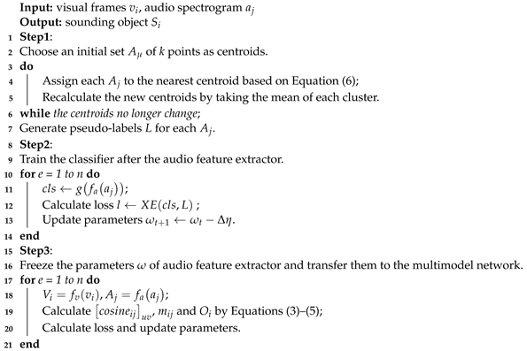
And The overall training process of the algorithm is as Algorithm 1 shows.

Algorithm 1: Sound Promotion Method (SPM)

2.4. Dataset

The MUSIC (Multimodal Sources of Instrument Combinations) dataset [18] contains 714 untrimmed videos of musical solos and duets, covering 11 classes of musical instruments. To demonstrate the effectiveness of our approach, we perform the same job as that in the Hu et al. [23] work, where the first five/two videos of each instrument category in solo/duet are used for testing, and the rest is used for training. Note that some videos are now not available on YouTube. We finally obtained 422 videos.

3. Results

3.1. Evaluation Metric

We adopt Consensus Intersection over Union (CIoU) and Area Under Curve (AUC) as the evaluation metrics to quantitatively analyze the results. The annotated bounding boxes are generated by a Faster RCNN network [24] to evaluate the positioning accuracy of the algorithm we proposed for the sounding object. The parameters of the Faster R-CNN model are obtained by training the public datasets, Open Image Datasets. Since this algorithm studies the detection of sounding objects, the instrument category in the Open Image Datasets were selected as the training set when training the Faster R-CNN model. During the training process, 15 musical instrument categories were selected from the Open Image Datasets, and a total of more than 30,000 images participated in the training of the Faster R-CNN model. These instrument categories include accordion, banjo, cello, drum, guitar, harp, harmonica, oboe, piano, saxophone, trombone, trumpet, violin, flute and horn. These 15 musical instrument categories basically cover the main categories of common musical instruments, so the target detection model Faster R-CNN trained using them can accurately identify musical instruments in the video and label relevant regions. Although these 15 categories do not include all musical instruments, they meet the criteria for this algorithm test. When detecting potential sounding objects in an actual video scene, many detection results are obtained. In order to filter out the most valuable results, we only keep the detection results with a confidence level higher than 90%, and manually clean up the remaining detection boxes. After such a screening process, the obtained target detection coordinates basically meet the requirements of the sound source localization test.

$$CIoU=\frac{{\sum }_{k=1}^K{\delta }_{k}Io{U}_k}{{\sum }_{k=1}^K{\delta }_k},$$

(7)

where $Io{U}_k$ is computed by the predicted sounding object area and annotated bounding box. The indicator is ${\delta }_k$ = 1 where the object is sounding, otherwise, it is 0.

3.2. Implementation Details

We divide each video equally into one-second clips with no intersection and randomly sample one image from the divided clips as the visual inputs, which is resized to 256 × 256. Then, we randomly crop them to a 224 × 224 size. As for audio, the inputs are first re-sampled into 16 KHz, then translated into a spectrogram via Short Time Fourier Transform (STFT). Log-Mel projection is performed over the spectrogram to better represent sound features. The audio and visual input from the same video clip are regarded as a positive sample. We use lightweight ResNet-18 [25] as audio and visual backbones. Our network is trained with the Adam optimizer with a learning rate of ${10}^{-4}$. Similar to the baselines [23], we pretrain the backbone of visual on ImageNet. In addition, we use $\theta$ = 0.65, $\tau$ = 0.03 and k = 11 as our network’s hyper-parameters. Finally, all these experiments are run on the computer with a GPU of 3080 10 G, and it takes about three weeks to complete the training stage.

3.3. Quantitative Results

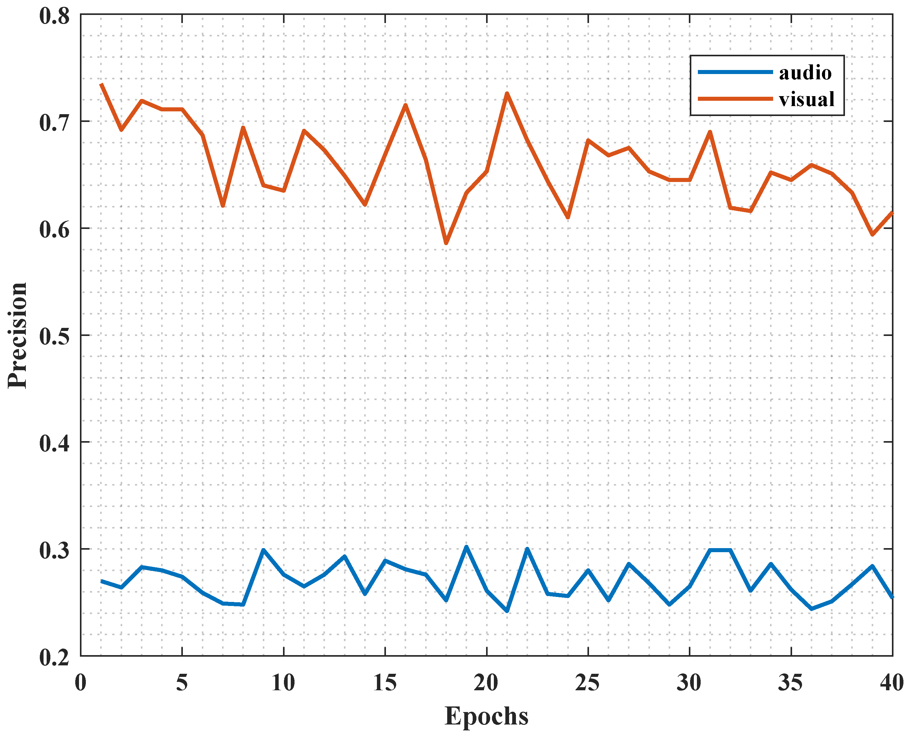
In this section, we compare our method (SPM) with the existing sound localization on the MUSIC dataset. First, in Figure 2, we show the reason why we separately improve the audio contribution. With the increase in training time, the accuracy of the audio classifier is much lower than that of the image classifier. According to the inference in [22], we can deduce the classifier performance of sound to show its contribution to the final result from the side. It was found that the accuracy of the image classifier was approximately 65%, while the accuracy of the audio classifier was only about 27%. This indicates that although both audio and images are used as inputs for network training, images contribute more to the final results, while audio has a lower level of involvement. Through in-depth analysis, it was discovered that the image feature extraction network, due to its pre-training, may become stuck in the vicinity of local optima, resulting in the phenomenon of “weak listening”. Thus, our method works in the freezing of the backbone of audio with a higher extraction rate to help it better learn the sound features.

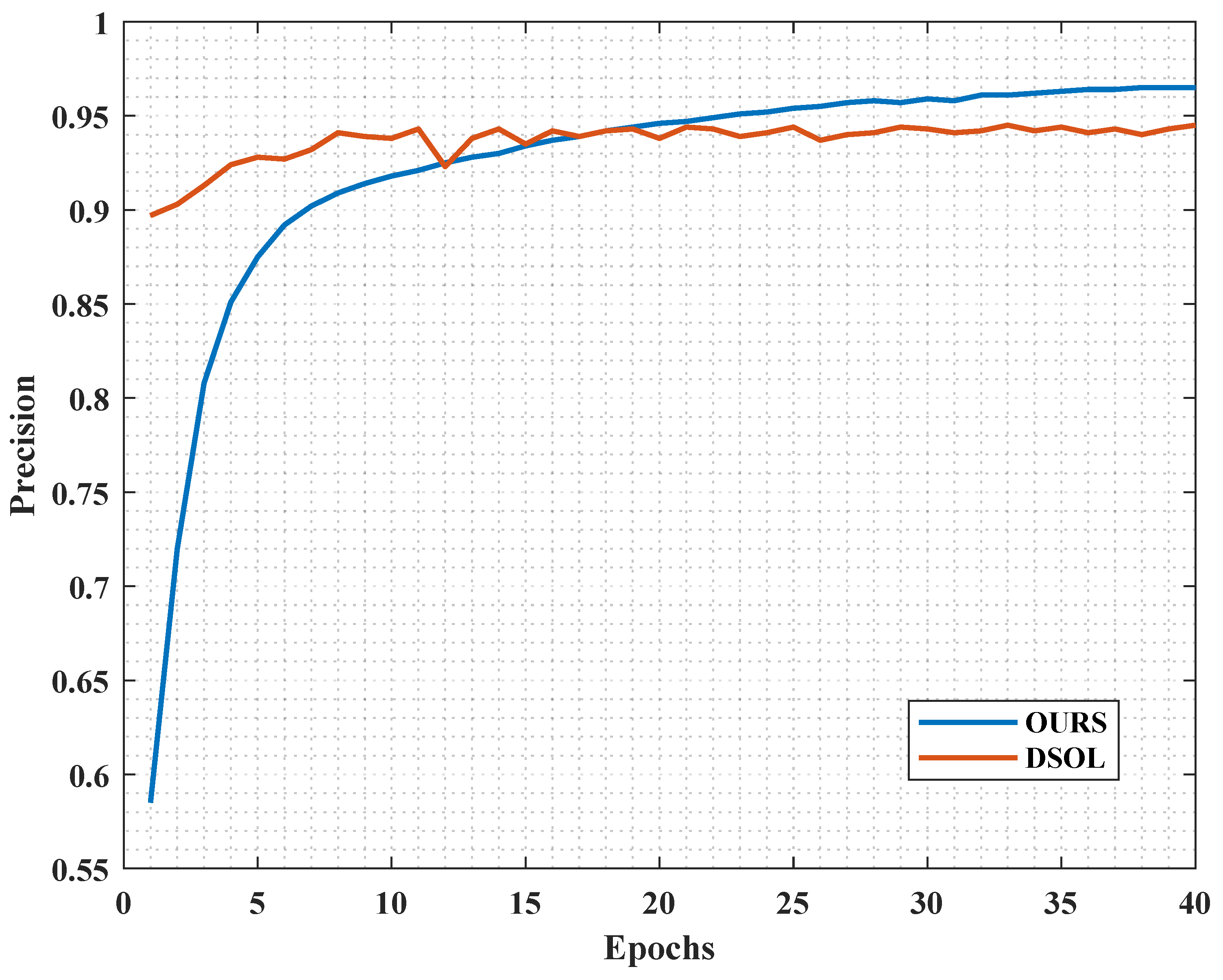
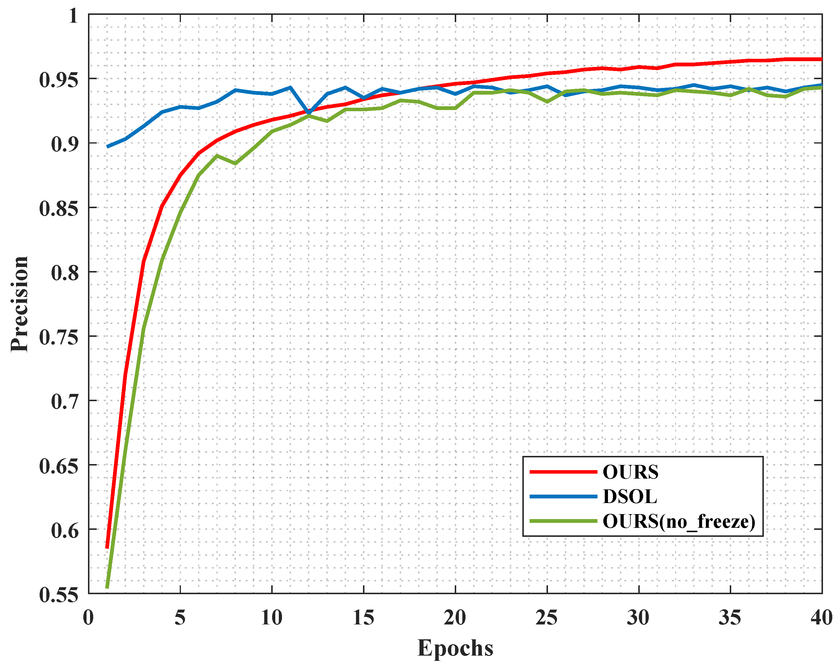
Then, in Figure 3, it can be observed that at the beginning of training, the DSOL algorithm performs well in overall accuracy because it is only pre-trained on images, ignoring audio information. However, as training progresses, the accuracy of DSOL starts oscillating and converges at 94.5%. In contrast, the convergence curve of our method shows a steady improvement trend. Although the overall accuracy is lower than that of DSOL at the beginning of training, with an increase in the number of iterations, the proposed algorithm gradually surpasses the comparative algorithm and ultimately achieves an accuracy of 96.5%. We believe that the multimodal fusion in the comparative network is mainly dominated by visual information. When the visual network’s extractor reaches its limit, the contribution of the audio extractor is lower, resulting in network oscillation. In contrast, for our algorithm, the audio extractor is frozen, and only the image extractor and the final classifier are trained. Due to the larger operatable space of image information, the overall network can progress towards the optimal point, avoiding the oscillation phenomenon. This indicates that increasing the contribution of audio features can lead to higher accuracy, bringing the network closer to the global optimum.

In

Table 1. Quantitative results on the MUSIC testset. Note that the CIoU reported in this table is [email protected], and our method outperforms the existing method on the test set.

Methods	CIoU(0.3)	AUC
Sound-of-Pixel [18]	8.1	11.8
Object-Sound [5]	3.7	10.2
DMC [17]	7.0	16.3
DSOL [23]	30.6	22.4
Ours	33.4	24.7

, it is shown that the method we propose outperforms the existing method on the test set. Due to the lack of data or the use of undisclosed optimization algorithms in the comparative algorithms during training, we cannot fully reproduce the experimental results from other papers. Therefore, we can only compare the accuracy provided in the other papers. Even so, the algorithm we propose still demonstrates better performance. When the CIoU is set to 0.3, in comparison to the best DSOL algorithm, our method improves by 2.8 percentage points and significantly surpasses the benchmark results of previous studies. We hypothesize that because the previous method did not have the operation like that of our model, the network could not escape from the local optimum when it converged. After the addition of our method, the network successfully converges to the better optimum, thereby improving the accuracy.

3.4. Qualitative Results

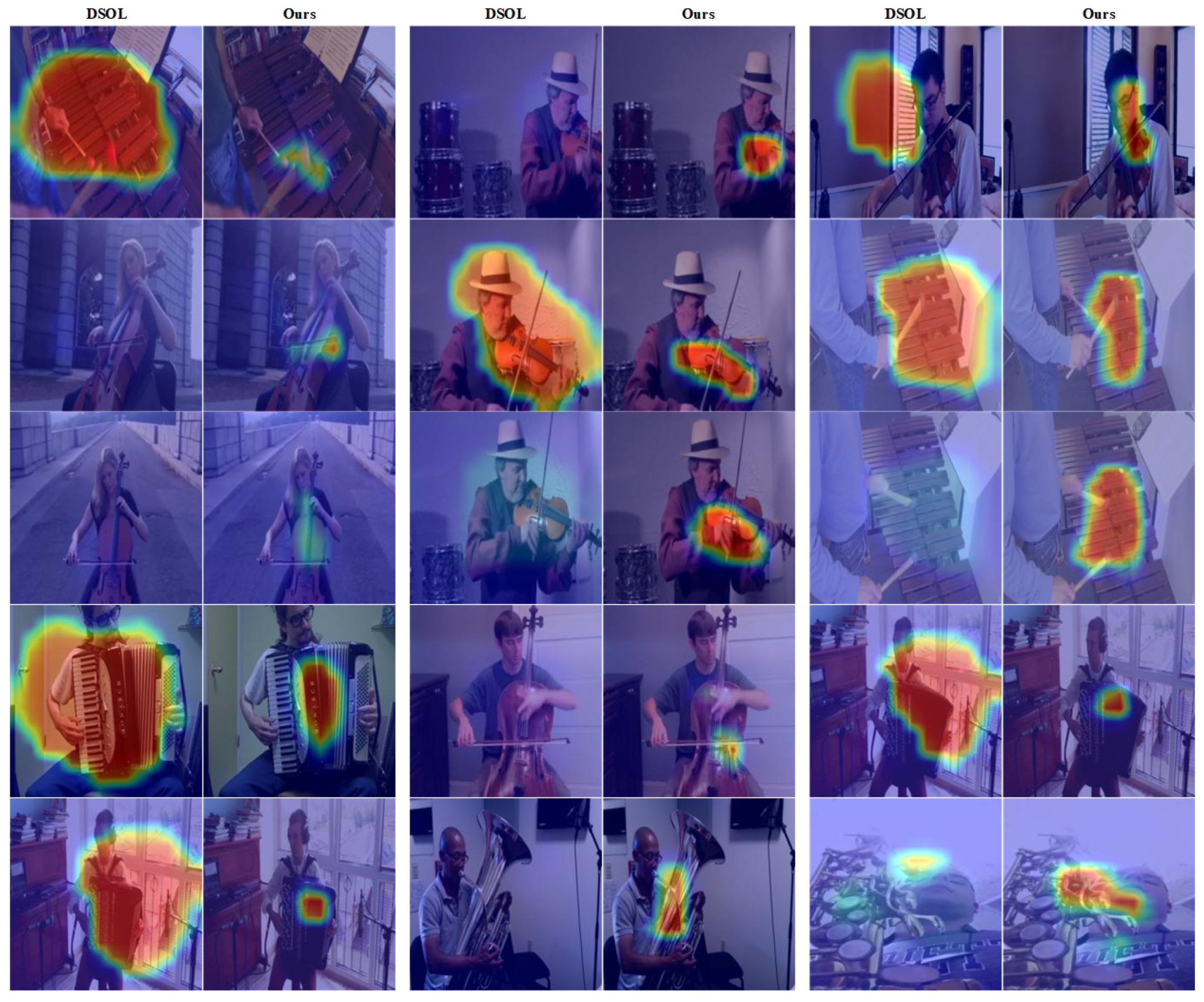
We visualize the prediction results in Figure 4, and we can find that our proposed method can produce a smaller and more precise heatmap output on the MUSIC dataset. Even in cases where the comparative algorithms fail to detect musical instruments, the algorithm we propose is still capable of detecting the position of the instruments, further confirming the effectiveness of our method. We hypothesize that, due to the frozen audio network and a large amount of redundant information that can be discarded in the image field, we keep the audio representation still and the network achieves better effect by adjusting image learning.

3.5. Alation Study

From the results shown in Figure 5, it can be observed that if only our algorithm is used for pre-training involving audio, the accuracy of the final network gradually approaches that of the DSOL algorithm, reaching only a 94.3% accuracy. A deep analysis of the curve reveals that after the first epoch of training, the accuracy of not freezing the audio extractor starts to decline compared to that of the proposed algorithm. This is because the performance of the audio extractor is affected, leading to an overall decrease in performance. The results eventually converging near the accuracy of DSOL also confirm the “weak listening” phenomenon mentioned above, where regardless of whether the audio extractor is involved in pre-training or not, the network tends to be biased towards visual dominance, suppressing the contribution of audio information. This validates the effectiveness of our algorithm once again.

The comparative results of the ablation experiments further demonstrate the superiority of the proposed algorithm and emphasize the importance of audio features. It is necessary to enhance their contribution by freezing the audio extractor in order to achieve better localization accuracy.

3.6. Additional Study

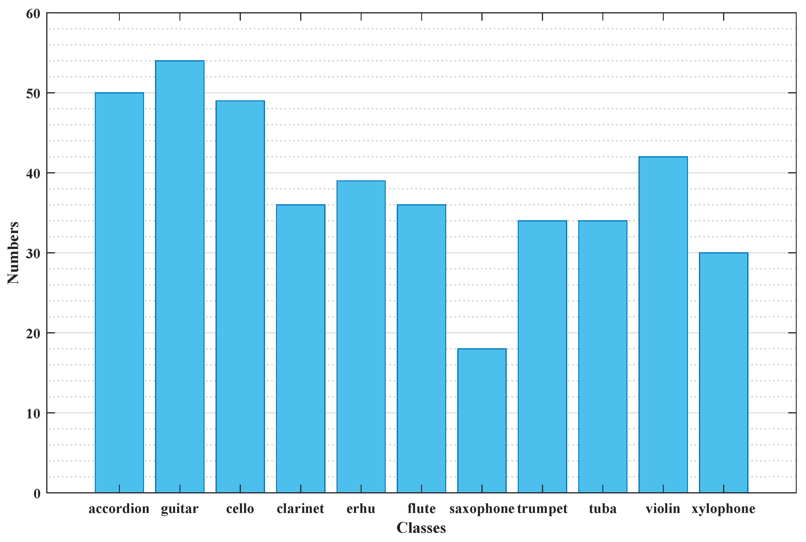
In the current situation, due to the large storage space occupied by large video datasets, there is no fixed packaging method available for download. Thus, the number of samples and the distribution of datasets that each person can obtain vary, which leads to biases in experimental results.

Figure 6 shows the number of samples in each category after removing five test samples from each category. It can be observed that the accordion, guitar, and cello have 50, 54, and 49 different samples, respectively, while the saxophone and xylophone only have 18 and 30 samples. This significant sample difference inevitably leads to dataset imbalance and can also affect the accuracy of the final results.

In response to the complexity of multimodal data augmentation, we attempted the following three experimental approaches to enhance the modal-specific features. By comparing these three different data augmentation methods, the optimal strategy can be determined, and further improvements can be made in the performance and accuracy of the multimodal sound source localization task.

Method A: Different frames are selected as image inputs within the same video while still using the original audio corresponding to the video for data augmentation.

Method B: The same frame of the video is selected as the image input, but the most similar audio to the original audio is found using Equation (6) as a replacement.

Method C: Different frames of the video are used as image inputs, and the most similar audio is found using Equation (6) as the corresponding audio.

Based on the results shown in Figure 7 and

Table 2. Comparison of three data enhancement methods.

Methods	Accordion	Acoustic_Guitar	Saxophone	Xylophone	All _Classes
A	35.0	35.4	33.6	33.7	34.4
B	35.7	36.1	33.8	34.3	35.6
C	36.2	35.8	34.1	34.5	35.8

, the CIoU under the three data augmentation methods and the comparative results can be observed. In Figure 7, the CIoU values for different categories under the three methods are depicted. Table 2 provides detailed data comparisons for the categories with the highest and lowest values, as well as the overall results.

For Method A, overall performance is inferior to that of Methods B and Method C, indicating that augmenting the image with the original audio yields inferior results compared to replacing the audio. This aligns with the expectations for traditional data augmentation methods, which do not apply well to multimodal tasks. The results demonstrate that merely enhancing the image while keeping the audio unchanged does not achieve optimal performance.

In comparison, there is little difference between Method B and Method C, but Method C slightly outperforms Method B. This suggests that better performance can be achieved by leveraging the diversity of images and audio and maintaining their correspondence. Method C, which comprehensively considers the characteristics of both image and audio in multimodal data augmentation, achieves favorable results.

4. Discussion

We investigate and explore the task of sound source localization in audio-visual correspondence learning, and we propose a self-supervised sound promotion method and achieves remarkable results. However, the algorithm we propose still has some limitations. The following are the issues that are worth further research and discussion: a. consideration of visual information temporal coherence factor; b. limitations of feature extraction algorithms. It is hoped that more and more researchers can enter this field to explore and help make the tasks related to audio-visual correspondence learning more universal and robust.

5. Conclusions

In this paper, we mine the inherent audiovisual contribution to the result and present a self-supervised sound promotion method to tackle the problem of low sound contribution. We validate our method on benchmarks showing great improvement. Experimental results indicate that our approach does increase the proportion of sound in the result, which also improves the accuracy of sound localization, as shown in Figure 4. Furthermore, future work should put emphasis on the more specific balance between vision and audio, because we believe in the following: the more balanced, the more accurate.