
Using Haze Level Estimation in Data Cleaning for Supervised Deep Image Dehazing Models

Abstract
:1. Introduction
- We introduced a haze level estimation (HLE) scheme in which a haze level indicator was devised based on the dark channel in ref. [1]. In ref. [1], it was observed that the haze level in an image is related to its dark channel. However, there is no further work on haze level estimation. To date, no such research has been conducted on using haze level information in a data set for SDID models. Thus, our HLE is a pioneering work in the SDID field.
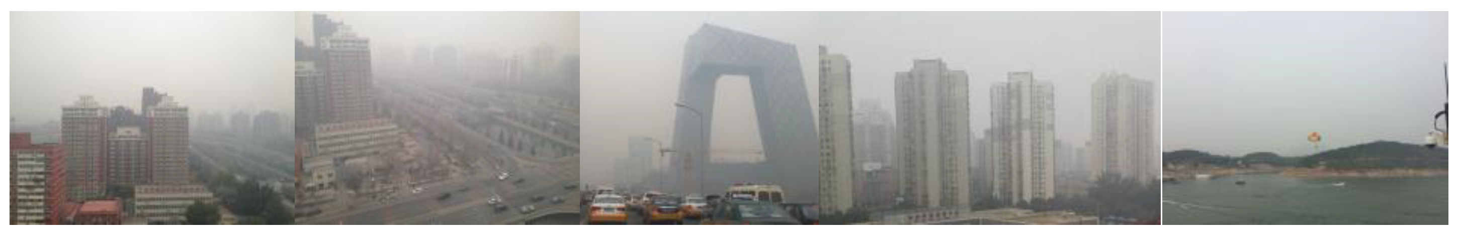
- We presented a data cleaning scheme based on the proposed HLE for SDID models. The haze level indicator is used to distinguish clear and hazy GT images in a data set. When a GT image is hazy, its corresponding hazy images are excluded together from the data set. The process to discard image pairs with hazy GT images is called data cleaning in this study. The experiment showed that the proposed data cleaning scheme can significantly improve the dehazing performance of SDID models. So far, no such work has been reported on SDID methods. Therefore, this paper is a contribution in this field.
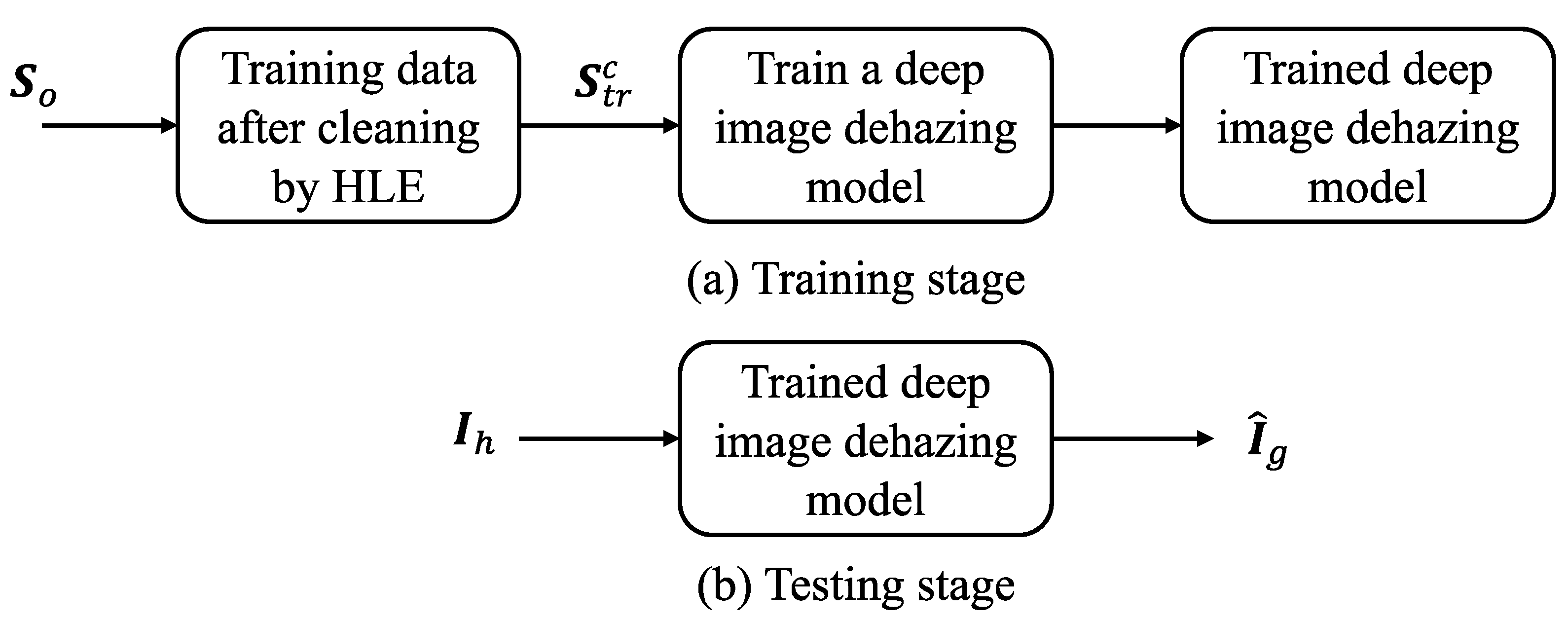
- We proposed an SDID framework that uses a data cleaning scheme to exclude image pairs with hazy GT images. This prevents an SDID model from learning an inappropriate mapping that degrades the dehazing performance. The proposed framework requires fewer training image pairs, yet achieves better dehazing performance. The framework can be easily applied to any SDID model. This is another contribution to the research community.
2. Haze Level Estimation and Data Cleaning
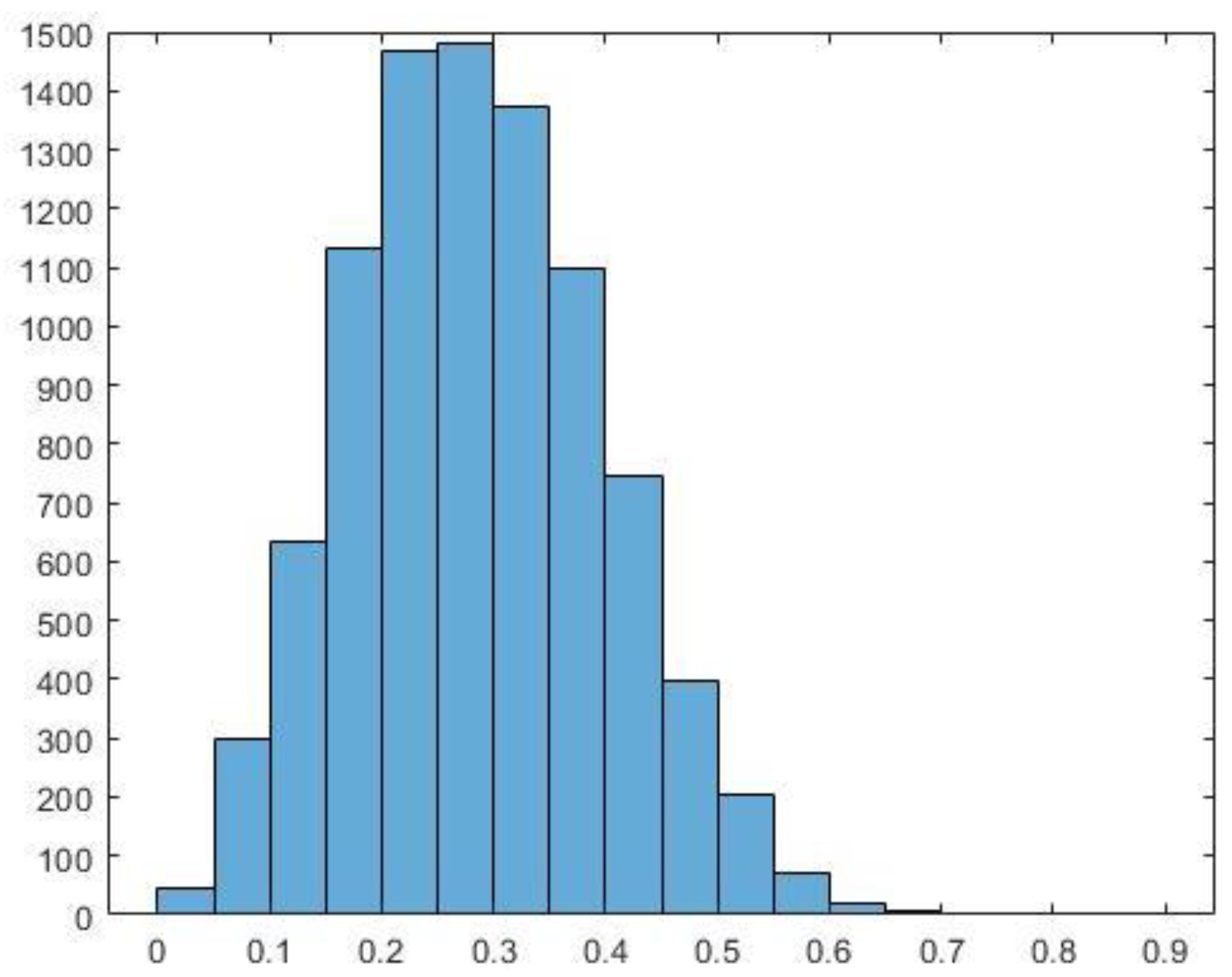
2.1. Haze Level Estimation
- Step 1.
- Obtain the dark channel using the minimum filter as below.where and is a window centered at .
- Step 2.
- Calculate the haze level indicator , a truncated mean of , as below.where is a user-defined threshold to exclude the pixel values from the calculation.
- Step 3.
- Check if the inequality holds, where is a user-defined threshold. If is true, then image is considered as clear. Otherwise, go to Step 4 for the second check.
- Step 4.
- Calculate the difference of , , and check if the inequality holds, where and . Notations and are user-defined thresholds. If is true, then image is considered as clear. Otherwise, it is hazy.
2.2. Application of the HLE to Data Cleaning
3. The Proposed SDID Framework
4. Results and Discussion
4.1. Determination of in the HLE
4.2. The GCAN Results for RESIDE Data Set
4.2.1. Objective Comparison
4.2.2. Subjective Comparison
4.3. The REFN Results for RESIDE Data Set
4.3.1. Objective Comparison
4.3.2. Subjective Comparison
4.4. The cGAN Results RESIDE Data Set
4.4.1. Objective Comparison
4.4.2. Subjective Comparison
4.5. The KeDeMa Results
4.5.1. The GCAN Results for KeDeMa Data Set
4.5.2. The REFN Results for KeDeMa Data Set
4.5.3. The cGAN Results KeDeMa Data Set
5. Conclusions and Further Research
Author Contributions
Funding
Data Availability Statement
Conflicts of Interest
References
- He, K.; Sun, J.; Tang, X. Single Image Haze Removal Using Dark Channel Prior. IEEE Trans. Pattern Anal. Mach. Intell. 2011, 33, 2341–2353. [Google Scholar] [CrossRef] [PubMed]
- Ju, M.; Ding, C.; Ren, W.; Yang, Y.; Zhang, D.; Guo, Y.J. IDE: Image Dehazing and Exposure Using an Enhanced Atmospheric Scattering Model. IEEE Trans. Image Process. 2021, 30, 2180–2192. [Google Scholar] [CrossRef] [PubMed]
- Zhu, Q.; Mai, J.; Shao, L. A Fast Single Image Haze Removal Algorithm Using Color Attenuation Prior. IEEE Trans. Image Process. 2015, 24, 3522–3533. [Google Scholar] [CrossRef]
- Fattal, R. Single image dehazing. ACM Trans. Graph. 2008, 27, 1–9. [Google Scholar] [CrossRef]
- Fattal, R. Dehazing Using Color-Lines. ACM Trans. Graph. 2014, 34, 1–14. [Google Scholar] [CrossRef]
- Xie, L.; Wang, H.; Wang, Z.; Cheng, L. DHD-Net: A Novel Deep-Learning-based Dehazing Network. In Proceedings of the 2020 International Joint Conference on Neural Networks (IJCNN), Glasgow, UK, 19–24 July 2020; pp. 1–7. [Google Scholar] [CrossRef]
- Li, B.; Peng, X.; Wang, Z.; Xu, J.; Feng, D. AOD-Net: All-in-One Dehazing Network. In Proceedings of the IEEE International Conference on Computer Vision (ICCV), Venice, Italy, 22–29 October 2017; pp. 4780–4788. [Google Scholar] [CrossRef]
- Zhu, H.; Cheng, Y.; Peng, X.; Zhou, J.T.; Kang, Z.; Lu, S.; Fang, Z.; Li, L.; Lim, J.-H. Single-Image Dehazing via Compositional Adversarial Network. IEEE Trans. Cybern. 2019, 51, 829–838. [Google Scholar] [CrossRef] [PubMed]
- Cai, B.; Xu, X.; Jia, K.; Qing, C.; Tao, D. DehazeNet: An End-to-End System for Single Image Haze Removal. IEEE Trans. Image Process. 2016, 25, 5187–5198. [Google Scholar] [CrossRef]
- Ren, W.; Liu, S.; Zhang, H.; Pan, J.; Cao, X.; Yang, M.-H. Single Image Dehazing via Multi-scale Convolutional Neural Networks. In Proceedings of the European Conference on Computer Vision, Amsterdam, The Netherlands, 11–14 October 2016; pp. 154–169. [Google Scholar]
- Yin, S.; Yang, X.; Wang, Y.; Yang, Y.-H. Visual Attention Dehazing Network with Multi-level Features Refinement and Fusion. Pattern Recognit. 2021, 118, 108021. [Google Scholar] [CrossRef]
- Jiao, L.; Hu, C.; Huo, L.; Tang, P. Guided-Pix2Pix+: End-to-end spatial and color refinement network for image dehazing. Signal Process. Image Commun. 2022, 107, 116758. [Google Scholar] [CrossRef]
- Zhang, H.; Patel, V.M. Densely Connected Pyramid Dehazing Network. In Proceedings of the IEEE Conference on Computer Vision and Pattern Recognition (CVPR), Salt Lake City, UT, USA, 18–23 June 2018; pp. 3194–3203. [Google Scholar] [CrossRef]
- Bai, H.; Pan, J.; Xiang, X.; Tang, J. Self-Guided Image Dehazing Using Progressive Feature Fusion. IEEE Trans. Image Process. 2022, 31, 1217–1229. [Google Scholar] [CrossRef]
- Li, P.; Tian, J.; Tang, Y.; Wang, G.; Wu, C. Deep Retinex Network for Single Image Dehazing. IEEE Trans. Image Process. 2020, 30, 1100–1115. [Google Scholar] [CrossRef]
- Chen, D.; He, M.; Fan, Q.; Liao, J.; Zhang, L.; Hou, D.; Yuan, L.; Hua, G. Gated Context Aggregation Network for Image Dehazing and Deraining. In Proceedings of the 2019 IEEE Winter Conference on Applications of Computer Vision (WACV), Waikoloa, HI, USA, 7–11 January 2019; pp. 1375–1383. [Google Scholar] [CrossRef]
- Li, R.; Pan, J.; Li, Z.; Tang, J. Single Image Dehazing via Conditional Generative Adversarial Network. In Proceedings of the CVPR Computer Vision and Pattern Recognition, Salt Lake City, UT, USA, 18–22 July 2018; pp. 8202–8211. [Google Scholar]
- Qu, Y.; Chen, Y.; Huang, J.; Xie, Y. Enhanced Pix2pix Dehazing Network. In Proceedings of the 2019 IEEE/CVF Conference on Computer Vision and Pattern Recognition (CVPR), Long Beach, CA, USA, 15–20 June 2019; pp. 8152–8160. [Google Scholar] [CrossRef]
- Huang, P.; Zhao, L.; Jiang, R.; Wang, T.; Zhang, X. Self-filtering image dehazing with self-supporting module. Neurocomputing 2020, 432, 57–69. [Google Scholar] [CrossRef]
- Dharejo, F.A.; Zhou, Y.; Deeba, F.; Jatoi, M.A.; Khan, M.A.; Mallah, G.A.; Ghaffar, A.; Chhattal, M.; Du, Y.; Wang, X. A deep hybrid neural network for single image dehazing via wavelet transform. Optik 2021, 231, 166462. [Google Scholar] [CrossRef]
- Zhao, D.; Mo, B.; Zhu, X.; Zhao, J.; Zhang, H.; Tao, Y.; Zhao, C. Dynamic Multi-Attention Dehazing Network with Adaptive Feature Fusion. Electronics 2023, 12, 529. [Google Scholar] [CrossRef]
- Cui, Z.; Wang, N.; Su, Y.; Zhang, W.; Lan, Y.; Li, A. ECANet: Enhanced context aggregation network for single image dehazing. Signal Image Video Process. 2022, 17, 471–479. [Google Scholar] [CrossRef]
- Agrawal, S.C.; Jalal, A.S. A Comprehensive Review on Analysis and Implementation of Recent Image Dehazing Methods. Arch. Comput. Methods Eng. 2022, 29, 4799–4850. [Google Scholar] [CrossRef]
- Gui, J.; Cong, X.; Cao, Y.; Ren, W.; Zhang, J.; Zhang, J.; Cao, J.; Tao, D. A Comprehensive Survey and Taxonomy on Single Image Dehazing Based on Deep Learning. ACM Comput. Surv. 2022, 55, 1–37. [Google Scholar] [CrossRef]
- Li, Y.; Miao, Q.; Ouyang, W.; Ma, Z.; Fang, H.; Dong, C.; Quan, Y. LAP-Net: Level-Aware Progressive Network for Image Dehazing. In Proceedings of the 2019 IEEE/CVF International Conference on Computer Vision (ICCV), Seoul, Korea, 27 October–2 November 2019; pp. 3275–3284. [Google Scholar] [CrossRef]
- Hong, M.; Xie, Y.; Li, C.; Qu, Y. Distilling Image Dehazing With Heterogeneous Task Imitation. In Proceedings of the 2020 IEEE/CVF Conference on Computer Vision and Pattern Recognition (CVPR), Seattle, WA, USA, 13–19 June 2020; pp. 3459–3468. [Google Scholar] [CrossRef]
- Wang, T.; Zhao, L.; Huang, P.; Zhang, X.; Xu, J. Haze concentration adaptive network for image dehazing. Neurocomputing 2021, 439, 75–85. [Google Scholar] [CrossRef]
- Li, B.; Ren, W.; Fu, D.; Tao, D.; Feng, D.; Zeng, W.; Wang, Z. Benchmarking Single-Image Dehazing and Beyond. IEEE Trans. Image Process. 2019, 28, 492–505. [Google Scholar] [CrossRef]
- Zhao, S.; Zhang, L.; Shen, Y.; Zhou, Y. RefineDNet: A Weakly Supervised Refinement Framework for Single Image Dehazing. IEEE Trans. Image Process. 2021, 30, 3391–3404. [Google Scholar] [CrossRef]
- Isola, P.; Zhu, J.-Y.; Zhou, T.; Efros, A.A. Image-to-Image Translation with Conditional Adversarial Networks. In Proceedings of the IEEE Conference on Computer Vision and Pattern Recognition (CVPR), Honolulu, HI, USA, 21–26 July 2017. [Google Scholar]
- Wang, Z.; Bovik, A.C.; Sheikh, H.R.; Simoncelli, E.P. Image Quality Assessment: From Error Visibility to Structural Similarity. IEEE Trans. Image Process. 2004, 13, 600–612. [Google Scholar] [CrossRef] [PubMed]
- Yeganeh, H.; Wang, Z. Objective Quality Assessment of Tone-Mapped Images. IEEE Trans. Image Process. 2013, 22, 657–667. [Google Scholar] [CrossRef] [PubMed]
- Nafchi, H.Z.; Shahkolaei, A.; Moghaddam, R.F.; Cheriet, M. FSITM: A Feature Similarity Index for Tone-Mapped Images. IEEE Signal Process. Lett. 2015, 22, 1026–1029. [Google Scholar] [CrossRef]
- Mittal, A.; Moorthy, A.K.; Bovik, A.C. No-Reference Image Quality Assessment in the Spatial Domain. IEEE Trans. Image Process. 2012, 21, 4695–4708. [Google Scholar] [CrossRef]
- Zhang, L.; Zhang, L.; Bovik, A.C. A Feature-Enriched Completely Blind Image Quality Evaluator. IEEE Trans. Image Process. 2015, 24, 2579–2591. [Google Scholar] [CrossRef]
- Min, X.; Zhai, G.; Gu, K.; Yang, X.; Guan, X. Objective Quality Evaluation of Dehazed Images. IEEE Trans. Intell. Transp. Syst. 2019, 20, 2879–2892. [Google Scholar] [CrossRef]
- Ma, K.; Liu, W.; Wang, Z. Perceptual evaluation of single image dehazing algorithms. In Proceedings of the 2015 IEEE International Conference on Image Processing (ICIP), Quebec City, QC, Canada, 27–30 September 2015; pp. 3600–3604. [Google Scholar] [CrossRef]


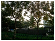
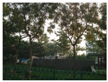
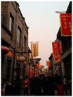
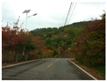
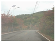
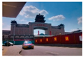
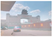
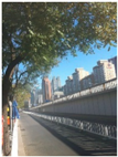
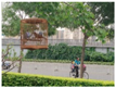
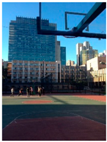
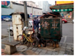
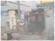
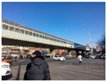
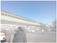
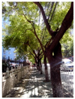
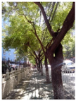
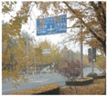
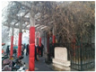
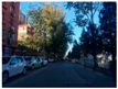
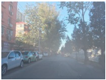
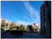
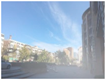
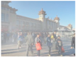
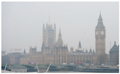
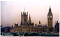
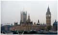
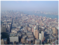
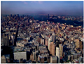
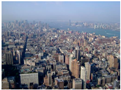
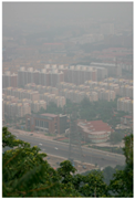
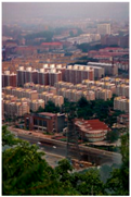
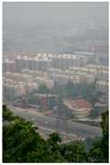
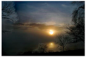
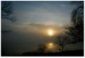
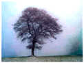
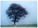
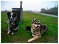
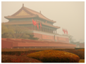
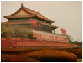
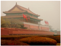
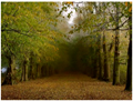
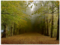
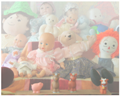
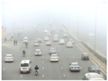
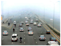
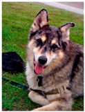
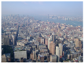
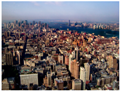
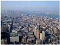
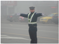
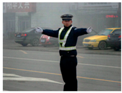
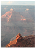
| Haze level indicator |  |  | 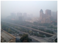 |
| 0.0252 | 0.2461 | 0.2312 | |
| 0.2528 | 0.2742 | 0.4661 | |
| 0.2276 | 0.0281 | 0.2349 | |
| Discrimination result | clear | clear | hazy |
| 0.025 | 0.05 | 0.075 | 0.1 | Original | |
| 104,440 | 113,295 | 136,570 | 166,425 | 313,950 | |
| 2984 | 3237 | 3902 | 4755 | 8970 | |
| 33.27% | 36.09% | 43.50% | 53.01% | 100% |
| Testing Set | ||||
|---|---|---|---|---|
| 10 K | 24.89 | 27.53 | 27.93 | 27.99 |
| 30 K | 24.96 | 27.56 | 28.01 | 28.07 |
| 50 K | 24.97 | 27.57 | 28.02 | 28.08 |
| Average | 24.94 | 27.55 | 27.99 | 28.04 |
| SSIM↑ | TMQI↑ | FSITM↑ | BRISQUE↑ | ILNIQE↓ | DHQI↑ | ↓ | |
|---|---|---|---|---|---|---|---|
| 0.91(2) | 0.92(2) | 0.73(2) | 20.46(1) | 21.31(2) | 54.96(2) | 1.83 | |
| 0.93(1) | 0.93(1) | 0.74(1) | 19.84(2) | 20.88(1) | 55.36(1) | 1.17 |
 |  = 0.11 |  PSNR = 28.09 |  PSNR = 28.69 | |
 |  21.03/0.26 |  26.23 |  28.70 | |
 |  14.22/0.36 |  25.61 | 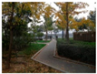 28.68 | |
 |  13.97/0.45 |  25.67 |  25.48 | |
 |  0.54 | 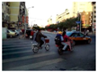 28.07 | 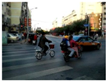 29.48 | |
 |  0.63 | 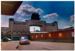 19.72 | 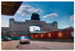 25.44 |
| Testing Set | ||||
|---|---|---|---|---|
| 10 K | 23.49 | 28.56 | 29.17 | 28.86 |
| 30 K | 23.43 | 28.57 | 29.19 | 28.87 |
| 50 K | 23.45 | 28.58 | 29.20 | 28.87 |
| Average | 23.45 | 28.57 | 29.19 | 28.87 |
| SSIM↑ | TMQI↑ | FSITM↑ | BRISQUE↑ | ILNIQE↓ | DHQI↑ | ↓ | |
|---|---|---|---|---|---|---|---|
| 0.93(2) | 0.93(2) | 0.77(2) | 16.28(1) | 19.78(1) | 52.67(2) | 1.67 | |
| 0.97(1) | 0.94(1) | 0.80(1) | 17.66(2) | 20.24(2) | 56.26(1) | 1.33 |
 |  = 0.15 |  PSNR = 23.05 |  PSNR = 31.50 | |
 |  0.25 | 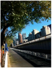 27.19 |  33.69 | |
 |  0.36 | 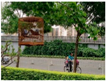 19.49 | 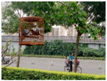 24.48 | |
 |  0.49 | 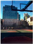 25.31 | 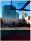 25.40 | |
 |  0.53 |  22.30 | 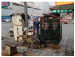 27.89 | |
 |  0.64 | 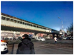 20.42 |  22.66 |
| Testing Set | ||||
|---|---|---|---|---|
| 10 K | 22.34 | 28.11 | 28.41 | 28.75 |
| 30 K | 22.33 | 28.14 | 28.45 | 28.78 |
| 50 K | 22.31 | 28.15 | 28.46 | 28.79 |
| Average | 22.33 | 28.13 | 28.44 | 28.77 |
| SSIM↑ | TMQI↑ | FSITM↑ | BRISQUE↑ | ILNIQE↓ | DHQI↑ | ↓ | |
|---|---|---|---|---|---|---|---|
| 0.91(2) | 0.89(2) | 0.74(2) | 10.99(1) | 20.39(1) | 57.90(1) | 1.50 | |
| 0.94 (1) | 0.94(1) | 0.76(1) | 11.88(2) | 33.77(2) | 57.75(2) | 1.50 |
 |  = 0.12 | 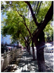 PSNR = 23.44 |  PSNR = 30.78 | |
 |  0.27 | 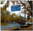 27.41 |  27.70 | |
 |  0.35 | 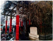 15.49 |  24.14 | |
 |  0.43 | 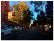 26.30 | 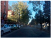 24.92 | |
 |  0.55 |  16.45 | 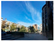 27.63 | |
 |  0.60 |  23.57 |  26.58 |
| BRISQUE↑ | ILNIQE↓ | DHQI↑ | ↓ | |
|---|---|---|---|---|
| 19.27(2) | 26.30(2) | 50.23(2) | 2 | |
| 17.28(1) | 25.93(1) | 50.90(1) | 1 |
 |  |  | |
 |  |  | |
 |  |  | |
 |  |  | |
 |  |  | |
 |  |  |
| BRISQUE↑ | ILNIQE↓ | DHQI↑ | ↓ | |
|---|---|---|---|---|
| 14.33(1) | 23.43(1) | 48.25(2) | 1.33 | |
| 16.97(2) | 26.11(2) | 51.06(1) | 1.67 |
 |  |  | |
 |  |  | |
 |  |  | |
 |  |  | |
 |  |  | |
 |  |  |
| BRISQUE↑ | ILNIQE↓ | DHQI↑ | ↓ | |
|---|---|---|---|---|
| 10.50(1) | 24.84(1) | 63.46(2) | 1.33 | |
| 29.97(2) | 37.81(2) | 55.31(1) | 1.67 |
 |  |  | |
 |  |  | |
 |  |  | |
 |  |  | |
 |  |  | |
 |  |  |
Disclaimer/Publisher’s Note: The statements, opinions and data contained in all publications are solely those of the individual author(s) and contributor(s) and not of MDPI and/or the editor(s). MDPI and/or the editor(s) disclaim responsibility for any injury to people or property resulting from any ideas, methods, instructions or products referred to in the content. |
© 2023 by the authors. Licensee MDPI, Basel, Switzerland. This article is an open access article distributed under the terms and conditions of the Creative Commons Attribution (CC BY) license (https://creativecommons.org/licenses/by/4.0/).
Share and Cite
Hsieh, C.-H.; Chen, Z.-Y. Using Haze Level Estimation in Data Cleaning for Supervised Deep Image Dehazing Models. Electronics 2023, 12, 3485. https://doi.org/10.3390/electronics12163485
Hsieh C-H, Chen Z-Y. Using Haze Level Estimation in Data Cleaning for Supervised Deep Image Dehazing Models. Electronics. 2023; 12(16):3485. https://doi.org/10.3390/electronics12163485
Chicago/Turabian StyleHsieh, Cheng-Hsiung, and Ze-Yu Chen. 2023. "Using Haze Level Estimation in Data Cleaning for Supervised Deep Image Dehazing Models" Electronics 12, no. 16: 3485. https://doi.org/10.3390/electronics12163485
APA StyleHsieh, C.-H., & Chen, Z.-Y. (2023). Using Haze Level Estimation in Data Cleaning for Supervised Deep Image Dehazing Models. Electronics, 12(16), 3485. https://doi.org/10.3390/electronics12163485