Spectral Clustering Approach with K-Nearest Neighbor and Weighted Mahalanobis Distance for Data Mining
Abstract
1. Introduction
- (1)
- In order to better capture the degree of linear correlation between the data, a correlation coefficient matrix is used as the weight to calculate the Mahalanobis distance, and then, the KNN method is used to construct the similarity matrix W.
- (2)
- The degree matrix D is calculated according to W and then a regularized Laplacian matrix L is constructed.
- (3)
- L is normalized and decomposed to obtain the feature space for clustering. This method fully considers the degree of linear correlation between data and achieves accurate clustering.
- (4)
- Multi-angle comparative experiments are conducted on artificial and UCI data sets to verify the superiority of MDLSC.
2. Related Information
2.1. Mahalanobis Distance
2.2. Similarity Matrix and Laplace Matrix
2.3. Spectral Clustering Algorithm
- (1)
- Construct a matrix W that can describe the similarity relationship between data through data samples. Construct Laplacian matrix L from degree matrix D and similarity matrix W.
- (2)
- Calculate and sort the eigenvalues and eigenvectors of Laplacian matrix L.
- (3)
- Take the eigenvectors corresponding to the first k eigenvalues after sorting, and arrange each vector in the column direction to form a new solution space.
- (4)
- On the new solution space, use the classical clustering algorithm (fuzzy clustering, K-means, etc.) for clustering and map the clustering result back to the original solution space.
3. Improved Spectral Clustering Algorithm
3.1. Mahalanobis Distance Spectral Clustering (M_SC) Algorithm
- (1)
- Calculate the Mahalanobis distance between each point and all other points, use the KNN algorithm to initialize it, and form similarity matrix W.
- (2)
- Calculate the regular Laplace matrix L = D−1/2(D − W) D−1/2; D is the degree matrix, that is, the sum of the elements of each row of similarity matrix W.
- (3)
- Calculate the eigenvectors corresponding to the first k eigenvalues of matrix L and place them in columns to form matrix U.
- (4)
- Unitize the row vectors in matrix U sequentially and then perform K-means clustering to obtain K clustering results.
3.2. Weighted Mahalanobis Distance Spectral Clustering (MDLSC) Algorithm
3.2.1. Weighted Mahalanobis Distance
The Weight Derivation Process of WMD
- (1)
- When performing principal component analysis, it is first necessary to standardize the data set D. Calculate the covariance matrix Γ of the standardized data D’; Γ is also the correlation coefficient matrix R, that is, Γ = R, and further obtain the characteristic root of Γ: λ1 ≥ λ2 ≥…≥ λp.
- (2)
- When performing principal component analysis on data, it is first necessary to standardize the data set D. Calculate the covariance matrix Γ of the standardized data D’; Γ is also the correlation coefficient matrix R, that is, Γ = R, and further obtain the the characteristic root of Γ: λ1 ≥ λ2 ≥……≥ λp.
- (3)
- Let Γ correspond to the unitized eigenvectors U1, U2, ……, Up and the matrix U = (U1, U2, ……, Up), formed by the eigenvectors. Suppose the diagonal matrix formed by characteristic roots {λ1, λ2, ……λp} is Λ = diag (λ1, λ2, ……λp); then, Λ = UT ΓU is established. Data set D’ is transformed into F = UT D’. Sample point X = ( x1, x2, ……, xp)T is converted into FX = UT X, and sample point Y = (y1, y2, ……, yp)T is converted into FY = UT Y.
- (4)
- Record F = (F1, F2, …, Fp)T, Fi = UiTD’, i = 1, 2, …, p and define ηi = λi/tr(Λ) as the variance contribution rate of Fi (i = 1,2,…,p) because Fi and Fj are independent of each other (i and j are integers between 1 and p); then, the Fi variance contribution rate can be used as the weight. The weight matrix recorded as the data set is W = diag(η1, η2,……, ηp); then, the correlation coefficient matrix of D’ after transformation is Γ = UTΓU. For any two sample points, the weight matrix is the same as the weight matrix of the data set and then the weighted Mahalanobis distance from FX to FY is expressed as shown in Equation (10):
- (5)
- According to Equation (12), UWUT = B in Equation (13). Since W = diag(η1, η2, …, ηp), Λ = diag (λ1, λ2, ……λp), ηi = λi/tr(Λ); thus, W = Λ/tr(Λ). Deduce B = U(Λ/tr(Λ))UT and, because Λ = UTΓU, Γ = UΛUT; then, B = Γ/tr(Λ) = R/tr(Λ). The weighted Mahalanobis distance formula for two samples X and Y is shown in Equation (11):
- (6)
- Since Γ = R, RΓ−1 = RR−1 = I; I is the identity matrix, and the final weighted Mahalanobis distance formula of samples X and Y is shown in Equation (12).
The Superiority of WMD
- (1)
- Covariance matrix: The covariance matrix is used to measure the degree of correlation and variation between different features. In the covariance matrix, the variance of each feature corresponds to its own importance, while the covariance measures the correlation between two features. If a feature has a higher variance, it has more variation in the data; thus, it can be considered to contribute more to the overall distance. Therefore, when using the covariance matrix as weights, the importance of features with a larger variance will be more prominent.
- (2)
- Correlation coefficient matrix: The correlation coefficient matrix measures the linear correlation between features, which removes the variance of the features themselves and focuses more on the relationship between features. The value range of the correlation coefficient is between −1 and 1, and the closer the absolute value is to 1, the stronger the linear relationship between the two features. If a feature has a strong linear relationship with other features, its corresponding value in the correlation coefficient matrix will be relatively large. When using the correlation coefficient matrix as a weight, the importance of features with strong linear relationships will be more prominent.
- (1)
- Considering the linear relationship between features: The correlation coefficient matrix captures the linear correlation between features. This is beneficial for spectral clustering since spectral clustering algorithms exploit the characteristic relationships of the data to build a similarity matrix. As a weight, the correlation coefficient matrix can better reflect the linear relationship between data points and provide a more accurate similarity measure.
- (2)
- The variance influence of the feature itself is removed: the correlation coefficient matrix eliminates the variance influence of the feature itself so that more attention is paid to the relationship between features when calculating the distance, without being affected by the variance of a single feature. This can reduce the dominance of large feature variance on the distance calculation and thus better capture the relative importance between features.
Calculation Steps of WMD
- (1)
- Calculate the mean of each variable di. i is an integer between 1 and p, the specific formula is shown in Equation (14):
- (2)
- Calculate the standard deviation of each variable di. i is an integer between 1 and p, the specific formula is shown in Equation (15):
- (3)
- Calculate the covariance matrix: Calculate the covariance among all variables in data set D. The covariance matrix is a p × p matrix where the (i, j)th element represents the covariance between the i-th variable and the j-th variable. Each element of the covariance matrix can be calculated using Equation (16):
- (4)
- Compute the correlation matrix: Calculate the correlation coefficient matrix using the covariance matrix. The correlation coefficient matrix is a p × p matrix where the (i, j)th element represents the correlation coefficient between the i variable and the j variable. Each element of the correlation coefficient matrix can be calculated using Equation (17):
- (5)
- The correlation coefficient matrix obtained through step (4) is R, and the weighted Mahalanobis distance between any two sample points can be calculated by Equation (14).
3.2.2. Construction of the Similarity Matrix
- (1)
- Calculate the weighted Mahalanobis distance between any two sample points, and the data constitute an n × n matrix (denoted as WM_matrix), which is a symmetric matrix.
- (2)
- Use the K-NN algorithm to traverse all data points and take the nearest k points of the distance (this distance is calculated by the Mahalanobis distance calculated in step (1)) of each data node vi as the nearest neighbor points, denoted as vi_KNN. vi_KNN is a set with k data nodes. Only the k points closest to the data node vi have a similarity greater than 0. Let Wij represent the similarity between the i-th data node vi and the j-th data node vj. When vj belongs to vi_KNN, then Wij > 0, and Wij is the weighted Mahalanobis distance from vi to vj; otherwise. Wij = 0. Experiments indicate that the effect of k being 3 and 5 is the same and the best, respectively. In order to reduce the amount of calculation, k is 3 in this paper. In order to ensure that the constructed similarity matrix W is symmetrical, it is constructed using method_B of KNN (see Section 2.2).
3.2.3. Construction of the Regularized Laplacian Matrix
- (1)
- Construct the degree matrix D. According to similarity matrix W (calculated in Section 3.2.2), degree matrix D is constructed. Degree matrix D is a diagonal matrix and its diagonal element D(i, i) represents the degree of node vi (that is, the number of edges connected to node vi). Graph G constructed in this paper is an undirected graph. D(i, i) can be calculated according to Equation (6).
- (2)
- Construct a standard Laplacian matrix L. According to the obtained similarity matrix W and degree matrix D, use Equation (7) to construct a standard Laplacian matrix L, i.e., L = D − W. The Laplacian matrix can provide important information about the graph structure and help cluster the data. The eigenvalues and eigenvectors of the Laplacian matrix can be obtained through spectral decomposition, thus realizing the core steps of the spectral clustering algorithm.
- (3)
- Construct a regularized Laplacian matrix. Symmetrically normalize L obtained by Equation (2), using Equation (18) to obtain a regularized Laplacian matrix L.
3.2.4. Steps for the MDLSC Algorithm
- (1)
- According to the steps in Section 3.2.1, calculate the weighted Mahalanobis distance of any two sample points and construct the weighted Mahalanobis distance matrix of the entire data set D.
- (2)
- According to the steps in Section 3.2.2, construct the similarity matrix W.
- (3)
- According to the steps in Section 3.2.3, construct the symmetric normalized Laplacian matrix L.
- (4)
- Perform spectral decomposition on L to obtain the eigenvectors corresponding to the first k smallest eigenvalues and place them according to column vectors to form matrix P. In order to make each new dimension reveal a cluster, the dimension k of the new space formed by P is usually set to the number of the last clustered clusters.
- (5)
- Unitize the row vector of matrix P and then perform K-means clustering to obtain the clustering result.
- (6)
- Calculate the clustering accuracy rate ACC, standard mutual confidence rate NMI, and purity and F1-Score.
3.2.5. Pseudocode for the MDLSC Algorithm
| Algorithm 1: MDLSC | |
| Input: Data D, Number of clusters K, Number of neighbors k | |
| Output: Clustering results K | |
| 1 | X = read(D)//read data into X |
| 2 | for xi to xn |
| 3 | di = get-mahalanobis( )//Calculate the weighted Mahalanobis distance of each//data point to other data points and store to di-matrix |
| 4 | KNN (di-matrix) = Wk //Use the KNN algorithm to mark the nearest k data points in the di-matrix to get Wk, here k = 3. |
| 5 | W = (Wk +WT)/2, Wk is transposed with WT //Calculate the Similarity matrix |
| 6 | D = diagonal sum of W //Calculate the Degree matrix |
| 7 | L = D-W //Calculate a standard Laplacian matrix L |
| 8 | L = D−1/2 L D−1/2 //Calculate the symmetric normalized Laplacian matrix |
| 9 | Calculate the first k smallest eigenvectors p1, p2, …, pk of L//the value of k is the same as the number of clusters |
| 10 | form p1, p2, …, pk into matrix P, |
| 10 | normalize P so that the norm of each row of p is 1.//data normalization |
| 11 | for (i = 1; i < = n; i++) |
| 12 | Taking each row vector yi in P as a data point, K-mean(yi) |
| 13 | Update data point labels |
| 14 | return K clustering results |
3.2.6. Algorithm Time Complexity Analysis
4. Experimental Results and Analysis
4.1. Data Set Description
4.2. Evaluation Metrics
4.3. Experimental Results and Analysis
4.3.1. Experiment on Artificial Data Sets
4.3.2. Experiment on UCI Data Set
4.4. Experimental Results and Analysis
5. Conclusions and Future Work
Author Contributions
Funding
Data Availability Statement
Conflicts of Interest
References
- Wang, J.; Wang, S.; Deng, Z. Several Problems in Cluster Analysis Research. Control Decis. 2012, 27, 8. [Google Scholar]
- Lei, X.; Xie, K.; Lin, F.; Xia, Z. An Efficient Clustering Algorithm Based on K-means Local Optimality. J. Softw. 2008, 19, 1683–1692. [Google Scholar] [CrossRef]
- Liu, Z.; Wu, P.; Wu, Y. Research on three spectral clustering algorithms and their applications. Comput. Applicat. Res. 2017, 34, 1026–1031. [Google Scholar]
- Miguel, C. On the diameter of the commuting graph of the matrix ring over a centrally finite division ring. Linear Algebra Its Applicat. 2016, 509, 276–285. [Google Scholar] [CrossRef]
- Zhou, X.; Ma, H.; Gu, J.; Chen, H.; Deng, W. Parameter adaptation-based ant colony optimization with dynamic hybrid mechanism. Eng. Appl. Artif. Intell. 2022, 114, 105139. [Google Scholar] [CrossRef]
- Zhang, J.M.; Sheny, X. Review on spectral methods for clustering. In Proceedings of the 2015 34th Chinese Control Conference (CCC), Hangzhou, China, 28–30 July 2015; pp. 3791–3796. [Google Scholar]
- Che, W.F.; Feng, G.C. Spectral clustering: A semi-supervised approach. Neuro Comput. 2012, 77, 119–228. [Google Scholar]
- Zhao, Y.C.; Zhang, S.C. Generalized Dimension-Reduction Frame work for Recent-Biased Time Series Analysis. IEEE Trans. Knowl. Data Eng. 2006, 18, 231–244. [Google Scholar] [CrossRef]
- Langone, R.; Mall, R.; Alzate, C.; Suykens, J.A.K. Kernel Spectral Clustering and Applications; Unsupervised Learning Algorithms; Springer International Publishing: Berlin/Heidelberg, Germany, 2016. [Google Scholar]
- Shi, B.; Guo, Y.; Hu, Y.; Yu, J. Multi-scale spectral clustering algorithm. Comput. Eng. Applicat. 2011, 47, 128–132. [Google Scholar]
- Fisher, D.H. Knowledge acquisition via incremental conceptual clustering. Machine Learn. 1987, 2, 139–172. [Google Scholar] [CrossRef]
- Shi, J.; Malik, J.M. Normalized cuts and image segmentation. IEEE Trans. Pattern Anal. Mach. Intell. 2000, 22, 888–905. [Google Scholar]
- Ng, A.Y.; Jordan, M.I.; Weiss, Y. On spectral clustering: Analysis and an algorithm. In Proceedings of the 14th International Conference on Neural Information Processing Systems: Natural and Synthetic, Vancouver, BC, Canada, 3–8 December 2001. [Google Scholar]
- Kong, W.Z.; Sun, Z.H.; Yang, C.; Sun, C. Automatic spectral clustering based on eigengap and orthogonal eigenvectors. Chin. J. Electron. 2010, 38, 1880–1885. [Google Scholar]
- Zhao, X.X.; Zhou, Z.P. A Semi-Supervised Spectral Clustering Algorithm Combining Sparse Representation and Constraint Transfer. J. Intell. Syst. 2018, 13, 855–862. [Google Scholar]
- Jia, Y.; Liu, H.; Hou, J.; Kwong, S.; Zhang, Q. Multi-view spectral clustering tailored tensor low-rank representation. IEEE Trans. Circuits Syst. Video Technol. 2021, 31, 4784–4797. [Google Scholar] [CrossRef]
- Wang, L.; Feng, B.L.; Cheng, J.L. Density -sensitive spectral clustering. Acta Electron. Sin. 2007, 35, 1577–1581. [Google Scholar]
- Wang, N.; Li, X. Active Semi-Supervised Spectral Clustering Algorithm Based on Supervised Information Characteristics. J. Electron. 2010, 38, 172–176. [Google Scholar]
- Wang, X.Y.; Ding, S.F.; Jia, W.K. Active constraint spectral clustering based on Hessian matrix. Soft Comput. 2020, 24, 2381–2390. [Google Scholar] [CrossRef]
- Klein, D.; Kamvar, S.D.; Manning, C.D. From Instance-Level Constraints to Space-Level Constraints: Making the Most of Prior Knowledge in Data Clustering; Stanford University: Stanford, CA, USA, 2002. [Google Scholar]
- Wu, L.; Wen, G.; Tong, T.; Tan, M.L.; Du, T.-T. Spectral clustering algorithm combining local PCA and k-nearest neighbors. Comput. Eng. Design 2019, 40, 2204–2210. [Google Scholar]
- Tao, X.; Wang, R.T.; Chang, R.; Huang, B.; Zhu, Q. Spectral Clustering Algorithm Based on Low Density Segmentation Density Sensitive Distance. Chin. J. Automat. 2020, 46, 1479–1495. [Google Scholar]
- Ge, J.; Yang, G. Density Adaptive Neighborhood Spectral Clustering Algorithm Based on Shared Nearest Neighbors. Comput. Eng. 2021, 47, 116–123. [Google Scholar] [CrossRef]
- Du, T.; Wen, G.; Wu, L.; Tong, T.; Tan, M. Spectral clustering algorithm based on local covariance matrix. Comput. Eng. Applicat. 2019, 148–154, 176. [Google Scholar]
- Yang, X. Research on Imbalanced Data Undersampling Method Based on Spectral Clustering. Comput. Digit. Eng. 2021, 49, 2305–2309+2330. [Google Scholar]
- Lu, G.; Lin, Z.; Yan, S.; Sun, J.; Yu, Y.; Ma, Y. Robust recovery of subspace structures by low-rank representation. IEEE Trans. Pattern Anal. Mach. Intell. 2012, 35, 171–184. [Google Scholar] [CrossRef] [PubMed]
- Elhamifar, E.; Vidal, R. Sparse subspace clustering. In Proceedings of the 2009 IEEE Computer Society Conference on Computer Vision and Pattern Recognition (CVPR), Miami, FL, USA, 20–25 June 2009; pp. 2790–2797. [Google Scholar]
- Sun, S. Subspace Clustering and Its Application; Xi’an University of Architecture and Technology: Xi’an, China, 2016. [Google Scholar]
- Kim, J.H.; Choi, J.H.; Park, Y.H.; Leung, C.K.S.; Nasridinov, A. KNN-SC: Novel spectral clustering algorithm using k-nearest neighbors. IEEE Access 2021, 9, 152616–152627. [Google Scholar] [CrossRef]
- Zhang, X.; Li, J.; Yu, H. Local density adaptive similarity measurement for spectral clustering. Patt. Recognit. Lett. 2011, 32, 352–358. [Google Scholar] [CrossRef]
- Nataliani, Y.; Yang, M.S. Powered Gaussian kernel spectral clustering. Neural Comput. Applicat. 2019, 31, 557–572. [Google Scholar] [CrossRef]
- Berahmand, K.; Mohammadi, M.; Faroughi, A.; Mohammadiani, R.P. A novel method of spectral clustering in attributed networks by constructing parameter-free affinity matrix. Cluster Comput. 2022, 25, 869–888. [Google Scholar] [CrossRef]
- Jiang, Z.; Liu, X. Adaptive KNN and graph-based auto-weighted multi-view consensus spectral learning. Informat. Sci. 2022, 609, 1132–1146. [Google Scholar] [CrossRef]
- Yin, L.; Li, M.; Chen, H.; Deng, W. An Improved Hierarchical Clustering Algorithm Based on the Idea of Population Reproduction and Fusion. Electronics 2022, 11, 2735. [Google Scholar] [CrossRef]
- Ren, Z.; Zhen, X.; Jiang, Z.; Gao, Z.; Li, Y.; Shi, W. Underactuated control and analysis of single blade installation using a jackup installation vessel and active tugger line force control. Mar. Struct. 2023, 88, 103338. [Google Scholar] [CrossRef]
- Song, Y.; Zhao, G.; Zhang, B.; Chen, H.; Deng, W.Q.; Deng, Q. An enhanced distributed differential evolution algorithm for portfolio optimization problems. Eng. Appl. Artif. Intell. 2023, 121, 106004. [Google Scholar] [CrossRef]
- Sun, Q.; Zhang, M.; Zhou, L.; Garme, K.; Burman, M. A machine learning-based method for prediction of ship performance in ice: Part I. ice resistance. Mar. Struct. 2022, 83, 103181. [Google Scholar] [CrossRef]
- Li, X.; Zhao, H.; Deng, W. BFOD: Blockchain-based privacy protection and security sharing scheme of flight operation data. IEEE Internet Things J. 2023. [Google Scholar] [CrossRef]
- Yu, Y.; Tang, K.; Liu, Y. A fine-tuning based approach for daily activity recognition between smart homes. Appl. Sci. 2023, 13, 5706. [Google Scholar] [CrossRef]
- Yu, C.; Gong, B.; Song, M.; Zhao, E.; Chang, C.I. Multiview Calibrated Prototype Learning for Few-shot Hyperspectral Image Classification. IEEE Trans. Geosci. Remote Sens. 2022, 60, 5544713. [Google Scholar] [CrossRef]
- Chen, H.; Wang, T.; Chen, T.; Deng, W. Hyperspectral Image Classification Based on Fusing S3-PCA, 2D-SSA and Random Patch Network. Remote Sens. 2023, 15, 3402. [Google Scholar] [CrossRef]
- Huang, C.; Zhou, X.; Ran, X.; Wang, J.; Chen, H.; Deng, W. Adaptive cylinder vector particle swarm optimization with differential evolution for UAV path planning. Eng. Appl. Artif. Intell. 2023, 121, 105942. [Google Scholar] [CrossRef]
- Xie, C.; Zhou, L.; Ding, S.; Liu, R.; Zheng, S. Experimental and numerical investigation on self-propulsion performance of polar merchant ship in brash ice channel. Ocean Eng. 2023, 269, 113424. [Google Scholar] [CrossRef]
- Cai, J.; Ding, S.; Zhang, Q.; Liu, R.; Zeng, D.; Zhou, L. Broken ice circumferential crack estimation via image techniques. Ocean Eng. 2022, 259, 111735. [Google Scholar] [CrossRef]
- Zhu, G.; Huang, S.; Yuan, C.; Huang, Y.H. SCoS: Design and Implementation of Parallel Spectral Clustering Algorithm Based on Spark. Chin. J. Comput. 2018, 41, 868–885. [Google Scholar]
- Bai, L.; Zhao, X.; Kong, Y.; Zhang, Z.; Shao, J.; Qian, Y. Review of Spectral Clustering Algorithms Research. Comput. Eng. Applicat. 2021, 57, 15–26. [Google Scholar]
- Chen, D.; Liu, J. Joint Learning of k-means and Spectral Clustering Based on Multiplicative Update Rule. J. Nanjing Univ. (Nat. Sci. Ed.) 2021, 57, 177–188. [Google Scholar]
- Li, M.; Zhang, J.; Song, J.; Li, Z.; Lu, S. A clinical-oriented non severe depression diagnosis method based on cognitive behavior of emotional conflict. IEEE Trans. Comput. Soc. Syst. 2022, 10, 131–141. [Google Scholar] [CrossRef]
- Duan, Z.; Song, P.; Yang, C.; Deng, L.; Jiang, Y.; Deng, F.; Jiang, X.; Chen, Y.; Yang, G.; Ma, Y.; et al. The impact of hyperglycaemic crisis episodes on long-term outcomes for inpatients presenting with acute organ injury: A prospective, multicentre follow-up study. Front. Endocrinol. 2022, 13, 1057089. [Google Scholar] [CrossRef] [PubMed]
- Jin, T.; Zhu, Y.; Shu, Y.; Cao, J.; Yan, H.; Jiang, D. Uncertain optimal control problem with the first hitting time objective and application to a portfolio selection model. J. Intell. Fuzzy Syst. 2022, 44, 1585–1599. [Google Scholar] [CrossRef]
- Li, M.; Zhang, W.; Hu, B.; Kang, J.; Wang, Y.; Lu, S. Automatic assessment of depression and anxiety through encoding pupil-wave from HCI in VR scenes. ACM Trans. Multimed. Comput. Commun. Appl. 2022. [Google Scholar] [CrossRef]
- Chen, M.; Shao, H.; Dou, H.; Li, W.; Liu, B. Data augmentation and intelligent fault diagnosis of planetary gearbox using ILoFGAN under extremely limited sample. IEEE Trans. Reliab. 2022, 1–9. [Google Scholar] [CrossRef]
- Zhou, X.; Cai, X.; Zhang, H.; Zhang, Z.; Jin, T.; Chen, H.; Deng, W. Multi-strategy competitive-cooperative co-evolutionary algorithm and its application. Inf. Sci. 2023, 635, 328–344. [Google Scholar] [CrossRef]
- Chen, H.; Chen, Y.; Wang, Q.; Chen, T.; Zhao, H. A New SCAE-MT Classification Model for Hyperspectral Remote Sensing Images. Sensors 2022, 22, 8881. [Google Scholar] [CrossRef]
- Chen, T.; Song, P.; He, M.; Rui, S.; Duan, X.; Ma, Y.; Armstrong, D.G.; Deng, W. Sphingosine-1-phosphate derived from PRP-Exos promotes angiogenesis in diabetic wound healing via the S1PR1/AKT/FN1 signalling pathway. Burn. Trauma 2023, 11, tkad003. [Google Scholar] [CrossRef]
- Li, Y.; Xiang, G. A Linear Discriminant Analysis Classification Algorithm Based on Mahalanobis Distance. Comput. Simulat. 2006, 23, 86–88. [Google Scholar]
- Yan, Z.; Zhang, Z.; Wang, Y.; Jin, Y.; Yan, T. Improved Deep Embedding Clustering Algorithm Based on Weighted Ma-halanobis Distance. J. Comput. Applicat. 2019, 39, 122–126. [Google Scholar]
- Cai, J.; Xie, F.; Zhang, Y. A New Fuzzy Clustering Algorithm Based on Mahalanobis Distance Feature Weighting. Comput. Eng. Applicat. 2012, 48, 422. [Google Scholar]
- Ma, Y.; Li, X.; Xue, S. A Fusion Algorithm of Spectral Clustering and Quantum Clustering Based on Manifold Distance Kernel. J. Northwest Normal Univ. (Nat. Sci. Ed.) 2023, 59, 37–46. [Google Scholar]
- Fan, J.; Deng, X.; Liu, Y. A Spectral Clustering Algorithm Based on Fréchet Distance. J. Guangdong Univ. Technol. 2023, 40, 39–44. [Google Scholar]
- Trillos, N.G.; Little, A.; McKenzie, D.; Murphy, J.M. Fermat Distances: Metric Approximation, Spectral Convergence, and Clustering Algorithms. arXiv 2023, arXiv:2307.05750. [Google Scholar]
- Zhang, Y.; Fang, K. Introduction to Multivariate Statistical Analysis; Science Press: Beijing, China, 1982. [Google Scholar]
- Fiedler, M. Algebraic connectivity of graphs. Czechoslovak Math. J. 1973, 23, 298–305. [Google Scholar] [CrossRef]
- Pang, Y.; Xie, J.; Nie, F.; Li, X. Spectral clustering by joint spectral embedding and spectral rotation. IEEE Trans. Cybernet. 2018, 50, 247–258. [Google Scholar] [CrossRef]
- Cai, X.; Dai, G.; Yang, L. A Survey of Spectral Clustering Algorithms. Comput. Sci. 2008, 35, 14–18. [Google Scholar]
- Cai, D.; He, X.; Han, J. Document clustering using locality preserving indexing. IEEE Trans. Knowl. Data Eng. 2005, 17, 1624–1637. [Google Scholar] [CrossRef]
- Strehl, A.; Ghosh, J. Cluster ensembles—A knowledge reuse framework for combining multiple partitions. J. Mach. Learn. Res. 2002, 3, 583–617. [Google Scholar]
- Wen, G. Research on Spectral Clustering Method for High-Dimensional Data; Guangxi Normal University: Guangxi, China, 2022. [Google Scholar] [CrossRef]
- Zhang, M. Research on the Evaluation Index of Symbolic Data Clustering; Shanxi University: Taiyuan, China, 2013. [Google Scholar]
- He, J. Spectral Clustering Algorithm for Improved Similarity Measurement. J. Guilin Inst. Aerospace Eng. 2017, 22, 123–127. [Google Scholar]




| Data Sets | Sample | Feature | Number of Clusters |
|---|---|---|---|
| Aggregation | 789 | 2 | 7 |
| Flame | 241 | 2 | 2 |
| Jain | 374 | 2 | 2 |
| Path-based | 301 | 2 | 3 |
| Spiral | 313 | 2 | 3 |
| Data Sets | Sample | Feature | Number of Clusters |
|---|---|---|---|
| Glass | 215 | 9 | 6 |
| Wine | 178 | 13 | 3 |
| Iris | 150 | 4 | 3 |
| Vehicle | 752 | 18 | 4 |
| Data Sets | Evaluation Metrics | Kernel SC | LSR | K-Means | NJW | MDLSC | M_SC |
|---|---|---|---|---|---|---|---|
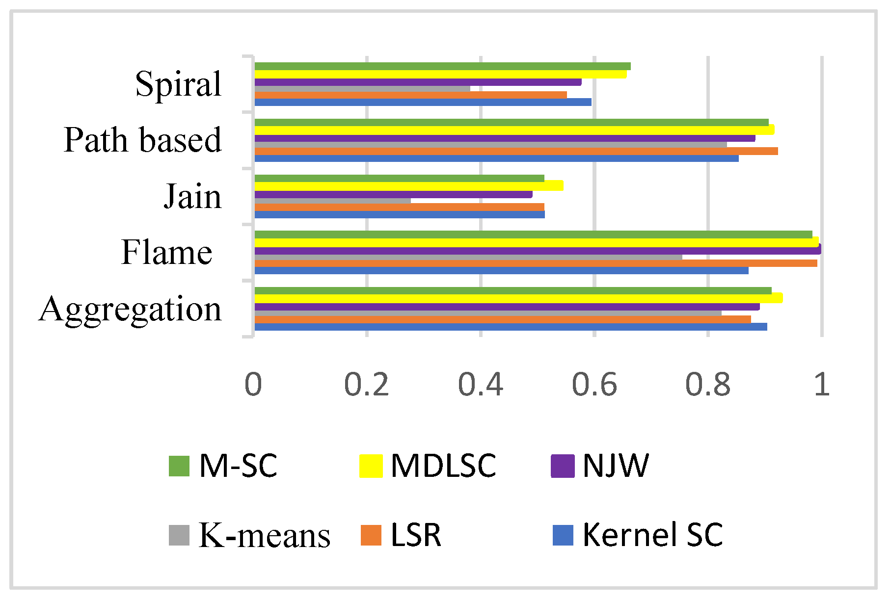
| Aggregation | ACC | 0.9035 | 0.8753 | 0.8238 | 0.888 | 0.928 | 0.9112 |
| NMI | 0.9088 | 0.8621 | 0.8421 | 0.9392 | 0.9492 | 0.8594 | |
| Purity | 0.8327 | 0.8461 | 0.8052 | 0.8327 | 0.8329 | 0.8314 | |
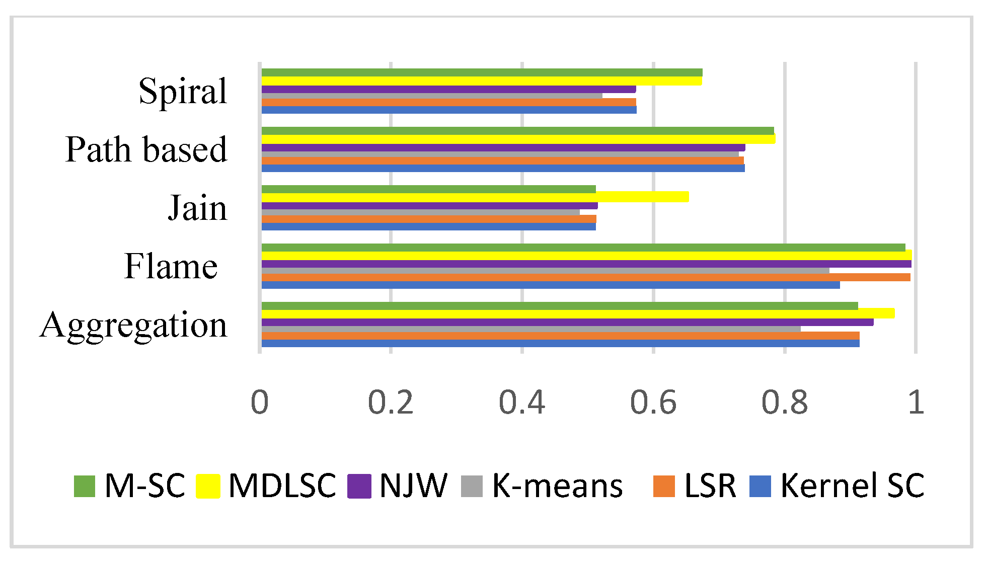
| F1-Score | 0.9136 | 0.914 | 0.8238 | 0.9328 | 0.9651 | 0.9112 | |
| Flame | ACC | 0.8708 | 0.9916 | 0.7541 | 0.9958 | 0.9916 | 0.9833 |
| NMI | 0.9259 | 0.9354 | 0.4534 | 0.9633 | 0.9875 | 0.899 | |
| Purity | 0.875 | 1 | 0.85 | 0.9958 | 1 | 0.9916 | |
| F1-Score | 0.8837 | 0.9916 | 0.8676 | 0.9909 | 0.9916 | 0.9833 | |
| Jain | ACC | 0.5124 | 0.512 | 0.2769 | 0.4879 | 0.5425 | 0.512 |
| NMI | 0.1108 | 0.1108 | 0.0468 | 0.1108 | 0.1492 | 0.1234 | |
| Purity | 0.1469 | 0.1637 | 0.0738 | 0.1469 | 0.1936 | 0.1892 | |
| F1-Score | 0.512 | 0.5123 | 0.4876 | 0.5123 | 0.6517 | 0.512 | |
| Path-based | ACC | 0.8533 | 0.923 | 0.8333 | 0.88 | 0.9133 | 0.9066 |
| NMI | 0.7148 | 0.7204 | 0.6622 | 0.7941 | 0.7951 | 0.8115 | |
| Purity | 0.6521 | 0.6254 | 0.4965 | 0.4552 | 0.6721 | 0.6366 | |
| F1-Score | 0.7392 | 0.7373 | 0.73 | 0.7373 | 0.7833 | 0.7833 | |
| Spiral | ACC | 0.5946 | 0.5519 | 0.381 | 0.5743 | 0.6538 | 0.6634 |
| NMI | 0.6358 | 0.6684 | 0.6176 | 0.6703 | 0.6995 | 0.7039 | |
| Purity | 0.802 | 0.8557 | 0.8218 | 0.8429 | 0.8461 | 0.8743 | |
| F1-Score | 0.5738 | 0.5734 | 0.5217 | 0.5707 | 0.6714 | 0.6743 |
Disclaimer/Publisher’s Note: The statements, opinions and data contained in all publications are solely those of the individual author(s) and contributor(s) and not of MDPI and/or the editor(s). MDPI and/or the editor(s) disclaim responsibility for any injury to people or property resulting from any ideas, methods, instructions or products referred to in the content. |
© 2023 by the authors. Licensee MDPI, Basel, Switzerland. This article is an open access article distributed under the terms and conditions of the Creative Commons Attribution (CC BY) license (https://creativecommons.org/licenses/by/4.0/).
Share and Cite
Yin, L.; Lv, L.; Wang, D.; Qu, Y.; Chen, H.; Deng, W. Spectral Clustering Approach with K-Nearest Neighbor and Weighted Mahalanobis Distance for Data Mining. Electronics 2023, 12, 3284. https://doi.org/10.3390/electronics12153284
Yin L, Lv L, Wang D, Qu Y, Chen H, Deng W. Spectral Clustering Approach with K-Nearest Neighbor and Weighted Mahalanobis Distance for Data Mining. Electronics. 2023; 12(15):3284. https://doi.org/10.3390/electronics12153284
Chicago/Turabian StyleYin, Lifeng, Lei Lv, Dingyi Wang, Yingwei Qu, Huayue Chen, and Wu Deng. 2023. "Spectral Clustering Approach with K-Nearest Neighbor and Weighted Mahalanobis Distance for Data Mining" Electronics 12, no. 15: 3284. https://doi.org/10.3390/electronics12153284
APA StyleYin, L., Lv, L., Wang, D., Qu, Y., Chen, H., & Deng, W. (2023). Spectral Clustering Approach with K-Nearest Neighbor and Weighted Mahalanobis Distance for Data Mining. Electronics, 12(15), 3284. https://doi.org/10.3390/electronics12153284


