Towards System-Level Simulation of a Miniature Electromagnetic Energy Harvester Model

Abstract

Energy harvesting, a solution to provide a lifetime power supply to wireless sensor nodes, has attracted widespread attention in the last two decades. An energy harvester collects ambient energy, e.g., solar, thermal, or vibration energy, and transforms it into electrical energy. In this work, we work on an electromagnetic energy harvester model, which is composed of four magnets oscillating along a coil. Such a device converts the vibrational energy into electrical energy. We reproduce the electromagnetic energy harvester model in finite element-based software. In order to include this model in a system-level simulation, the methodology of extracting a look-up table-based equivalent circuit model is presented. Such an equivalent circuit model enables the interaction of the electromagnetic energy harvester model with both electrical and mechanical compact models at the system-level. Furthermore, the matrix interpolation-based and algebraic parameterization-based parametric model order reduction methods are suggested for speeding up the generation of the equivalent circuit model and the design optimization process with respect to magnet dimensions. The efficiencies of these two methods are investigated and compared.

1. Introduction

The ‘Fourth Industrial Revolution’, also known as ‘Industry 4.0’, is a concept that describes the rapid change in technology and industries as a result of growing interconnectivity and intelligent automation. It is driven by emergent and disruptive intelligence and information technologies that significantly influence the industry, social, and environmental sustainable development [1]. Industry 4.0 technologies, including but not limited to artificial intelligence, big data analytics, cloud computing and the internet of things (IoT), improve the levels of current production efficiencies, quality, and industrial system sustainability [2,3]. For example, different from traditional manufacturing practices, the IoT enables machine-to-machine communication and automates the production process. The production data are collected from the sensors and analyzed via big data analytics. The whole manufacturing system is integrated with increasing automation, communication, and self-monitoring even without requiring human involvement.

The key point of the example above is the IoT technique, which uses wireless devices to connect the machines digitally and uses sensors to monitor physical and environmental phenomena and exchange data. Numerous wireless devices form a wireless network for automation and data transmission in the manufacturing process. However, the battery-powered wireless nodes or sensors limit the operational time and performance of the system. Manual battery recharging may not be viable technically and economically. Therefore, various energy harvesting technologies, which are utilized to transform various types of ambient energy into electricity, have emerged as potential strategies to develop self-sustaining wireless networks since the 2000s [4,5]. For instance, piezoelectric, electrostatic, and electromagnetic energy harvesters are categorized as vibration-based energy harvesters, which convert vibrations in a sensor’s operating environment into electrical energy [6,7,8]. In this paper, we aim to present a case study of modeling and simulation of an electromagnetic energy harvester.

Numerical modeling and computer-based simulation enhance the energy harvesters’ design process. Simulating the numerical models reduces the cost of fabricating prototypes and thereby speeds up the design optimization process. In this work, we reproduce the electromagnetic energy harvester model [9] in the finite element method (FEM)-based software. It is found that the high computational costs of the finite element (FE) model are directly determined by the total number of elements. A refined mesh with a large number of elements makes the FE model less efficient to be used in system-level simulations. Therefore, the goal of this work is to provide strategies to speed up the simulation of the model, enable efficient parametric optimization, and realize the co-simulation with the control circuitry.

Recently, several advances of system-level modeling have been reported [10,11]. Different from the lumped-element equivalent circuit model constructed based on the derived analytical equations [10] and the macromodel extracted via system model identification method [11], in this contribution, we present the workflow of exporting a look-up table-based equivalent circuit model from an electromagnetic energy harvester model via the equivalent circuit extraction (ECE) technique [12,13]. This equivalent circuit model can be imported into the system-level simulation software for efficient simulations. The interconnection of the equivalent circuit to both electrical and mechanical components at the system-level is demonstrated.

However, the generation of the equivalent circuit model is based on a parametric solution of the full-order FE model and it is still time-consuming. To generate the compact models of electromagnetic devices, model order reduction techniques have been receiving a growing amount of interest in the last decades [14,15,16,17,18]. In addition, the authors in [19] implemented the parametric model order reduction (pMOR) method on electromagnetic systems to generate a parametric reduced-order model with parameterized material properties and boundary conditions. In this contribution, in order to speed up the parametric studies of a geometrically parameterized electromagnetic energy harvester model, we adapted two alternative pMOR methods for effective parametric studies of the reduced-order model (ROM). One method is referred to as the matrix-interpolation-based pMOR method suggested by Panzer et al. [20]. The general framework of this pMOR method is that several values of the geometrical parameter are selected and the corresponding FE models are reduced via model order reduction methods, e.g., the Block Arnoldi algorithm from [21], and are noted as local ROMs. The parametric reduced-order model (pROM) is then interpolated on the basis of these local ROMs. The other method is introduced by Moosmann in [22,23], which enables the users to extract the geometrical parameter out of the system matrices of the FE full-order model (FOM) via algebraic parameterization. Then, the projection-based multivariate-moment matching pMOR method [24,25], which is successfully demonstrated for material properties and boundary conditions in thermal problems [26,27,28], can be applied directly. It is verified in this work that this method is also applicable to geometry parameters.

For the first time, in this work, we compare the computational efficiencies of these two pMOR methods and the performance of the pROMs. Both methods are first implemented on a two-dimensional (2D) single permanent magnet model, then on a three-dimensional (3D) electromagnetic energy harvester FE model. It should be noted that the precondition for both methods is that the topology of the mesh should be preserved when changing the geometry parameter. In this work, this is achieved via scaling the elements in the mesh. It is found that when the dimension of the FOM becomes sizeable, the method suggested by Moosmann encounters its limitation and the algebraic parameterization process requires substantial computational effort. Thereby, a new workflow for the algebraic parameterization process is suggested in this work.

The structure of this paper is as follows. In Section 2, the setups of the electromagnetic energy harvester model are introduced. The ECE technique and system-level simulation are presented in Section 3. Then, Section 4 introduces the parametric model order reduction methods utilized in this work. In Section 5, the numerical results of the pMOR methods applied to the electromagnetic energy harvester model are presented and discussed. The conclusion of this work and the outlook for future research are given in Section 6.

2. Case Study: Electromagnetic Energy Harvester

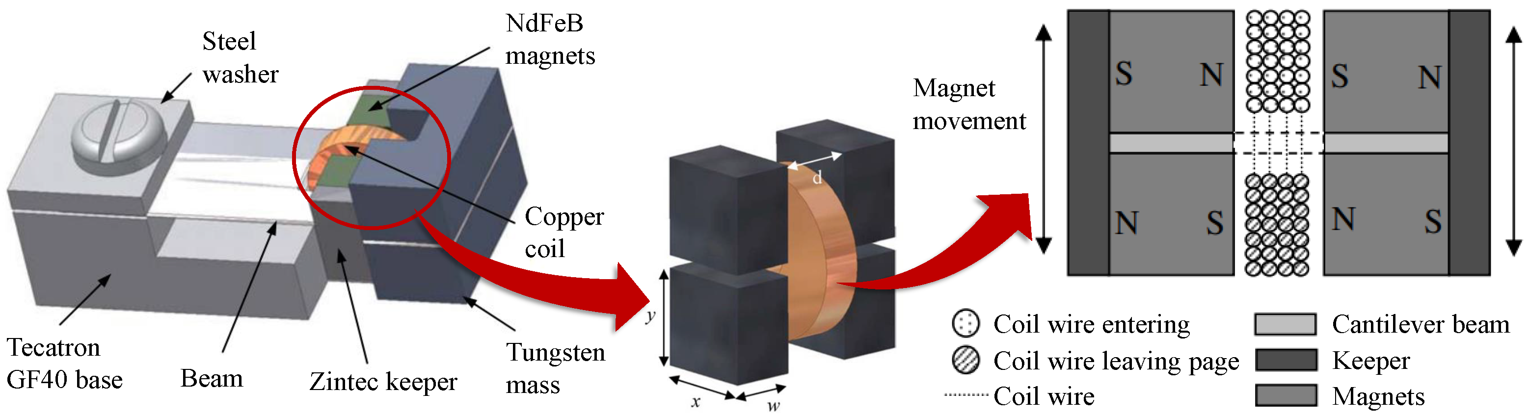
An electromagnetic energy harvester transforms vibrational mechanical energy from the environment into electrical energy. In this work, we reproduce the electromagnetic energy harvester model [9] in the FE software ANSYS Maxwell 3D [29]. Figure 1 illustrates the structure of the model. Four high-energy density sintered rare earth neodymium iron boron (NdFeB) magnets are arranged along with a copper coil. The characteristics of the materials used in the model are presented in

Table 1. Material properties of NdFeB and copper.

Material	Relative Permeability	Bulk Conductivity (S/m)	Magnetic Coercivity (A/m)	Mass Density (kg/m${}^3$)
NdFeB (Magnets)	1.099779	6.25 × 10${}^5$	8.9 × 10${}^5$	7400
Copper (Coil)	0.999991	5.8 × 10${}^7$	n.a.	8933

. Two magnets are attached to the top and bottom sides of a 0.1 mm thick cantilever beam on either side of the coil. The distance d between the magnets on two sides of the coil is 1 mm. The magnets are 1 × 1 × 1.5 mm${}^3$ in size and polarized along the edge w = 1.5 mm. The coil volume in the middle of the structure has an outside radius of 1.2 mm and an inside radius of 0.3 mm. The coil thickness is 0.5 mm. It is configured with 600 turns of 25 μm diameter copper wire. With this arrangement, a concentrated flux gradient through the stationary coil is produced as the magnets oscillate together with the cantilever. The changing magnetic field through the coil induces a voltage in the coil, which is utilized as a power supply.

In this work, four magnets and the coil were constructed as shown in Figure 2. The two magnets on each side of the coil were grouped and moved in a 9 × 4.8 × 8.2 mm${}^3$ motion band in the z-direction between −0.57 and 0.57 mm. The initial resting position was at −0.57 mm. In order to establish the oscillation of the magnets, a time-dependent force was applied to each group of magnets:

$$F\left(t\right)=m{\omega }^2{x}_0\cos \left(\omega t\right)$$

(1)

where m = 22.2 μg is the mass of two magnets, $\omega$ = 2$\pi f$ with f = 60 Hz is the excitation frequency and the designated oscillation amplitude is $x_0$ = 0.57 mm. The coil terminals, which were connected to an external circuit, were defined on the cross-section area of the coil. 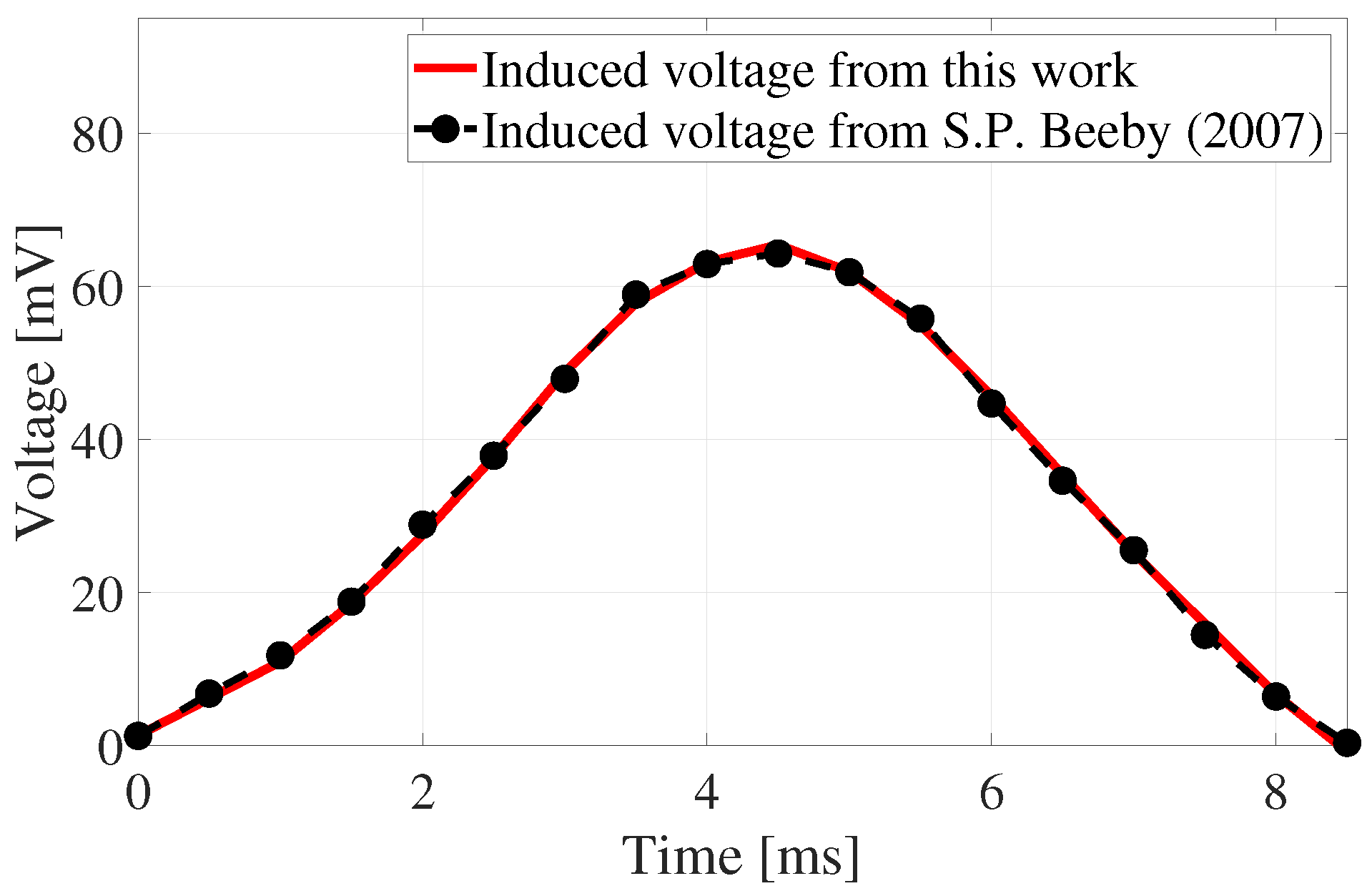In this case study, the external circuit was composed of a coil inductor, a 100 $\mathsf{\Omega }$ coil internal resistor, and a 10 G$\mathsf{\Omega }$ large load resistor. In this way, the open circuit voltage induced in the coil can be observed. There was no current/voltage excitation defined to the coil. More details of the model setups are given in [13]. Thereby, the induced voltage in the coil as obtained from this work is presented in Figure 3. The maximum voltage output during transient analysis is 65.4 mV, which is close to the simulation finding of 64 mV from [9] with a relative error of 2.2%.

3. Equivalent Circuit Extraction Technique

In the validated electromagnetic energy harvester model built in this work, the coil was connected to an external electrical circuit at the system-level, where the induced voltage output from the coil served as a voltage source. However, a total of 125,821 elements were generated in the mesh of the FE model. In each time point of the transient analysis, the model is remeshed in respect to the change of the position of the magnets. It took around 135 min to perform the transient simulation over the period of 8.5 ms with a time step 0.5 ms (Intel Core Processor (Broadwell, IBRS) 3.0 GHz, 64 GB RAM). Therefore, to reduce the computational cost, a compact model must be generated from the 3D FE electromagnetic energy harvester model for efficient system-level simulations. In this section, we will introduce the equivalent circuit extraction technique in ANSYS Maxwell 3D, which enables us to generate an equivalent circuit model from the original FE electromagnetic energy harvester model for fast simulations at the system-level [12,13].

However, due to technical reasons [12], the equivalent circuit model can be exported from a parametric solution with magnetostatic analysis, whereas in Section 2 a transient scheme was implemented. Thereby, the positions of the magnets were parameterized to represent the oscillation of the magnets already used in the transient analysis. By using Faraday’s law of induction [30], the induced voltage output was calculated via the obtained magnetic flux rate change through the coil:

$$EMF=-N·\frac{\Delta \mathsf{\Phi }}{\Delta t}$$

(2)

where N is the number of turns in the coil, $\Delta \mathsf{\Phi }$ is the change in the magnetic flux through the coil in each time step $\Delta t$. The negative sign in the equation indicates that the induced electromotive force ($EMF$) opposes the change in the magnetic flux.

The parametric simulation results were pre-calculated and saved as a look-up table in the equivalent circuit model (see Figure 4). In this look-up table, the positions of the magnets and the current in the coil were used as the inputs and the magnetic flux through the coil was the output. The interpolation method was deployed to calculate the magnetic flux outputs from those input values which were not listed in the parametric solution results-based look-up table. The equivalent circuit model was further able to be imported into the system-level simulation software and enable the connection to both electrical and mechanical circuits for real-time system-level simulations.

The system-level simulation tool ANSYS Twin Builder [31] can load the equivalent circuit model. In Figure 4, on the right-hand side of the equivalent circuit model, the dynamics of the harvester are imitated by lumped elements in the mechanical circuit. The inertia of the magnets is represented by the mass component. Position source, damping, and spring components determine the excitation applied to the magnets. On the left-hand side, a simple load circuit, which is composed of a load resistor and a coil inductor, is connected to the equivalent circuit model.

In the mechanical circuit, m = 22.2 μg is the mass component, which presents the mass of two magnets on one side of the coil. It is excited with an excitation frequency f = 60 Hz. The spring rate is calculated as:

$$k={\omega }^{2}m={\left(2\pi f\right)}^{2}m=3.16\mathrm{N}/\mathrm{m}$$

(3)

The excitation amplitude can be calculated as follows:

$$y_0=\frac{a_0}{{\omega }^2}=\frac{a_0}{{\left(2\pi f\right)}^2}=4.15\mathsf{\mu }\mathrm{m}$$

(4)

where $a_0$ = 0.59 m/s${}^2$ is the acceleration amplitude. In order to obtain the designated oscillation amplitude, the damping coefficient is chosen to be 6.8 × 10${}^{-5}$ Ns/m. Given a peak displacement amplitude of 0.57 mm, the quality factor of the harvester model becomes 137.3.

In the electrical circuit, the resistance of the load resistor is defined as 10 G$\mathsf{\Omega }$, which sets an open circuit condition. The induced voltage in the coil obtained from the equivalent circuit model is shown in Figure 5. The maximum voltage output is around 65.5 mV, which is close to the expected value of 64 mV. It could also be found in

Table 2. Computational time comparison between finite element model and equivalent circuit model (Intel Core Processor (Broadwell, IBRS) 3.0 GHz, 64 GB RAM).

	Model Generation Time	Simulation Period	Time Step	Computational Time
Finite element model	n.a.	8.5 ms	0.5 ms	135 min
Equivalent circuit model	244 min (325 groups of parametric solutions)	3.5 s	1 μs	19 s

that the computational time for the simulation of the equivalent circuit model is much faster than the finite element model. It took only 19 s to perform the simulation of the equivalent circuit model with a simulation period of 3.5 s and time step 1 μs, while it took around 135 min to run the simulation of the full-scale FE model with a simulation period of 8.5 ms and time step 0.5 ms.

Then, the parametric studies of the load resistance in the electrical circuit could be performed efficiently on the basis of the equivalent circuit model. As shown in Figure 6, the maximum power output of 4.28 μW is obtained when the load resistance matches the internal resistance of the coil.

4. Parametric Model Order Reduction

Although the equivalent circuit model enables efficient system-level simulation, generation of the equivalent circuit model required 244 min as shown in Table 2. This effort stems from the necessity to solve 325 parameter sets of the full-scale FE electromagnetic energy harvester model. In this case study, the position of the magnets was parameterized between −0.6 and 0.6 mm with a step size of 0.05 mm; the coil current is parameterized between −0.6 and 0.6 mA in steps of 0.1 mA.

For design optimization of the device, parametric studies of the original FE model with geometrical parameters are necessary. In this section, we therefore suggest using pMOR methods to reduce the computational effort of parametric studies. More specifically, pMOR methods will enable us to parameterize the geometrical parameters of the electromagnetic energy harvester model at the reduced-order model level. These parametric solutions calculated from the pROM can be saved as a look-up table, which can be used to construct the equivalent circuit model for system-level simulations. Moreover, the pROM can be transformed into a system-level model, e.g., a VHDL model, with conservative ports. This could be performed and must be validated in the future.

4.1. Finite Element Model

pMOR methods require system matrices of the FE model. To our best knowledge, there is no way to obtain the system matrices from ANSYS Maxwell 3D. Therefore, we implemented the model in ANSYS Mechanical APDL [32], where the system matrices could be obtained via the software ‘Model Reduction inside ANSYS’ [33].

In this case, the magnetostatic model was simulated without current input to the coil. Therefore, the system can be represented by the subset of Maxwell’s equations [34]:

$$\begin{array}{c}\hfill \nabla \times \mathrm{H}=\mathrm{J}\end{array}$$

(5)

$$\begin{array}{c}\hfill \nabla ·\mathrm{B}=0\end{array}$$

(6)

where $\mathrm{H}$ is the magnetic field intensity, $\mathrm{B}$ is the magnetic flux density and $\mathrm{J}$ = 0 is the applied source current. When permanent magnets are considered, a magnetization vector field $\mathrm{M}$ is introduced and it relates to the magnetic field intensity $\mathrm{H}$ and magnetic flux density $\mathrm{B}$ as follows:

$$\mathrm{B}={\mathsf{\mu }}_0(\mathrm{H}+\mathrm{M})$$

(7)

where ${\mathsf{\mu }}_0$ is the permeability of free space.

In ANSYS Mechanical APDL, the magnetostatic system can be solved by using either

• Magnetic scalar potential: the magnetic field intensity $\mathrm{H}$ can be expressed as a negative gradient of the scalar potential $\varphi$:

  $$\mathrm{H}=-\nabla \varphi$$

  (8)
  In Equation (7), replace $\mathrm{H}$ by Equation (8) and take Equation (7) into Equation (6):

  $$0=-\nabla ·{\mathsf{\mu }}_0\nabla \varphi +\nabla ·{\mathsf{\mu }}_0\mathrm{M}$$

  (9)
• Magnetic vector potential: the magnetic flux density $\mathrm{B}$ is defined as a curl of the vector potential $\mathrm{A}$:

  $$\mathrm{B}=\nabla \times \mathrm{A}$$

  (10)
  Replace $\mathrm{B}$ in Equation (7) by Equation (10) and take it into Equation (5), we obtain:

  $$0=-\nabla \times \frac{1}{{\mathsf{\mu }}_0}(\nabla \times \mathrm{A})+\nabla \times \mathrm{M}$$

  (11)

After finite element discretization, both Equations (9) and (11) can be written in the matrix form as follows:

$${\Sigma }_n:\left\{\begin{array}{c}0=K·x+B·u\hfill \\ y=C·x\hfill \end{array}\right.$$

(12)

where $K\in {\mathbb{R}}^{n\times n}$ is the coefficient matrix with dimension n. $B\in {\mathbb{R}}^{n\times m}$ is the input matrix with m inputs and $C\in {\mathbb{R}}^{p\times n}$ is the output matrix and it gives p outputs. x is the unknown state vector which contains the magnetic scalar potential $\varphi$ or vector potential $\mathrm{A}$. y is the output vector and $u=\left[\begin{array}{c}mag\_top\\ mag\_bot\end{array}\right]$ is the input vector, which is constructed by the coercive force properties of the permanent magnets and defines the polarization direction.

4.2. Matrix Interpolation Based pMOR

If a geometrical parameter l is introduced to the FE model, the system matrices will all become dependent on it. Then, the system in Equation (13) could be written in geometrical parameter-dependent form as follows:

$$\Sigma {\left(l\right)}_n:\left\{\begin{array}{c}0=K\left(l\right)·x+B\left(l\right)·u\hfill \\ y=C\left(l\right)·x\hfill \end{array}\right.$$

(13)

The matrix-interpolation-based pMOR method suggested by Panzer et al. [20] derives a pROM of such a FE model with geometrical parameters. In this subsection, we will briefly review and discuss this method. The following steps make up the basic framework for pMOR by matrix interpolation and will be applied to the case study in this work:

Step 1. k values of the geometrical parameter $l=\{l_1,l_2,\dots ,l_k\}$ are selected and the corresponding full-scale models are reduced and stored in the database $\mathit{DB}=\{{\Sigma }_{r,1},{\Sigma }_{r,2},\dots ,{\Sigma }_{r,k}\}$:

$${\Sigma }_{r,i}\left\{\begin{array}{c}0=\underset{K_{r,i}}{\underbrace{{V_i}^T{K}_i{V}_i}}·z_i+\underset{B_{r,i}}{\underbrace{{V_i}^T{B}_i}}·u\hfill \\ y=\underset{C_{r,i}}{\underbrace{C_i{V}_i}}·z_i\hfill \end{array}\right.$$

(14)

where $K_{r,i}\in {\mathbb{R}}^{r\times r}$, $B_{r,i}\in {\mathbb{R}}^{r\times m}$ and $C_{r,i}\in {\mathbb{R}}^{p\times r}$ are the reduced system matrices at those discrete parameter values $l_i,i\in [1,k]$. $z_i\in {\mathbb{R}}^r$ are the corresponding reduced order state vectors. $V_i\in {\mathbb{R}}^{n\times r}$ with $r\ll n$ are the local projection matrices.

Step 2. These local ROMs are transformed into another set of generalized coordinates $z_i^{*}={\mathbf{T}}_i·z_i$ as follows:

$${\Sigma }_{r,i}^{*}\left\{\begin{array}{c}0=\underset{K_{r,i}^{*}}{\underbrace{{\mathbf{M}}_i{K}_{r,i}{\mathbf{T}}_i^{-1}}}·z_i^{*}+\underset{B_{r,i}^{*}}{\underbrace{{\mathbf{M}}_i{B}_{r,i}}}·u\hfill \\ y=\underset{C_{r,i}^{*}}{\underbrace{C_{r,i}{\mathbf{T}}_i^{-1}}}·z_i^{*}\hfill \end{array}\right.$$

(15)

where the transformation matrices are defined as ${\mathbf{T}}_i={\mathbf{R}}^T·V_i$ and ${\mathbf{M}}_i={\left(V_i^T·\mathbf{R}\right)}^{-1}$. Matrix $\mathbf{R}$ is constructed by performing the singular value decomposition (SVD) on the matrix pool of the local projection matrices $V_{all}$ and choosing the first r columns of U:

$$\mathbf{U}\Sigma {\mathbf{N}}^T=\mathrm{SVD}(\underset{V_{all}}{\underbrace{[V_1,V_2,\dots ,V_k]}})$$

(16)

$$\mathbf{R}=\mathbf{U}(:,1:r)$$

Step 3. The system matrices of the global pROM are constructed through a weighted interpolation method based on the system matrices obtained from the local ROMs ${\Sigma }_{r,i}^{*}=\{K_{r,i}^{*},B_{r,i}^{*},C_{r,i}^{*}\}$. In this work, the Lagrange interpolation strategy [35] was utilized to calculate the pROM with parameter l:

$$\Sigma {\left(l\right)}_r^{*}=\sum _{j=1}^k\frac{w\left(l\right)}{(l-l_i)w^{\prime }\left(l_i\right)}·{\Sigma }_{r,i}^{*}$$

(17)

where:

$$\left\{\begin{array}{c}w\left(l\right)=(l-l_1)(l-l_2)\cdots (l-l_k)\hfill \\ w^{\prime }\left(l_i\right)=(l_i-l_1)\cdots (l_i-l_{i-1})(l_i-l_{i+1})\cdots (l_i-l_k)\hfill \end{array}\right.$$

It should be noted that, in Step 1, the computational cost for generating a ROM from a static model is almost equivalent to its solution due to the fact that the local projection matrices $V_i$ are calculated via the modified Gram-Schmidt algorithm [36] on the term $-{K_i}^{-1}{B}_i$. However, the approach of matrix interpolation-based pMOR still reduces the computational time because the step of interpolating the local ROMs is faster than directly solving the static model at that discrete point.

In addition, the matrix interpolation-based pMOR method has an essential prerequisite that the mesh topology of the local FE models should be constant. In other words, the dimension of the local projection matrices should be the same. Otherwise, the SVD of the matrix pool will not be viable in Step 2. In this contribution, we implemented a scheme in ANSYS Mechanical APDL to scale the mesh elements to preserve the mesh topology. Other research related to matrix interpolation-based pMOR methods with changing mesh topology is given in [28,37,38,39].

4.3. Algebraic Parameterization-Based pMOR

Another pMOR method applicable to geometrically parameterized FE models is suggested in [22,23]. The authors introduced an approach for the algebraic parameterization of FE models with varying geometrical parameters. In this subsection, we shall introduce this method and indicate its limitation. We will suggest an improved workflow of this method in this paper.

Similar to matrix interpolation-based pMOR, this method is applicable only if the mesh topology, i.e., the matrix structure, remains unchanged. Varying the geometrical parameter could be achieved by scaling the size of the elements as shown in Figure 7.

This method follows the following steps:

Step 1. The geometrical parameter-dependent Equation (13) is extended to a parametric form:

$${\Sigma }_n\left\{\begin{array}{c}0=\underset{K(\frac{1}{\alpha },\alpha )}{\underbrace{(\frac{1}{\alpha }·K_{\frac{1}{\alpha }}+K_1+\alpha ·K_{\alpha })}}·x+B·u\hfill \\ y=C·x\hfill \end{array}\right.$$

(18)

where $\alpha$ is the scaling factor for the geometrical parameter l, e.g., the height of the magnets. The parameter-independent system matrices $K_{\frac{1}{\alpha }}$, $K_1$, and $K_{\alpha }\in {\mathbb{R}}^{n\times n}$ can be computed through the following numerical scheme:

$$\left[\begin{array}{c}{K}_{{\alpha }_1,i,j}\\ K_{{\alpha }_2,i,j}\\ K_{{\alpha }_3,i,j}\end{array}\right]=\left[\begin{array}{c}\frac{1}{{\alpha }_1}1{\alpha }_1\\ \frac{1}{{\alpha }_2}1{\alpha }_2\\ \frac{1}{{\alpha }_3}1{\alpha }_3\end{array}\right]\left[\begin{array}{c}{K}_{\frac{1}{\alpha },i,j}\\ K_{1,i,j}\\ K_{\alpha ,i,j}\end{array}\right]$$

(19)

where $K_{{\alpha }_1},K_{{\alpha }_2},K_{{\alpha }_3}$ are the system matrices snapshotted with different values of $l=\{l_1,l_2,l_3\}$. ${\alpha }_1=\frac{l_1}{l_1},{\alpha }_2=\frac{l_2}{l_1},{\alpha }_3=\frac{l_3}{l_1}$ are the identified scaling factors of the elements.

Step 2. Equation (19) is constructed and solved for each matrix entry, that is $n^2$ times. n is the dimension of the system matrix. The solution of $K_{\frac{1}{\alpha },i,j}$, $K_{1,i,j}$, and $K_{\alpha ,i,j}$ assembles the desired parameter-independent matrices.

Step 3. On the basis of Equation (18), the multivariate moment-matching-based pMOR method can be applied to generate a parametric ROM:

$${\Sigma }_r\left\{\begin{array}{c}0=\underset{K_r(\frac{1}{\alpha },\alpha )}{\underbrace{V^{T}K(\frac{1}{\alpha },\alpha )V}}·z+\underset{B_r}{\underbrace{V^{T}B}}·u\hfill \\ y=\underset{C_r}{\underbrace{CV}}·z\hfill \end{array}\right.$$

(20)

where $K_r\in {\mathbb{R}}^{r\times r}$, $B_r\in {\mathbb{R}}^{r\times m}$, and $C_r\in {\mathbb{R}}^{p\times r}$ are the reduced system matrices. $V\in {\mathbb{R}}^{n\times r}$ is a global projection matrix obtained by merging two local projection matrices of parameter $\frac{1}{\alpha }$ and $\alpha$. According to our previous research [28], for the parametric static model, the local projection matrices can be constructed by orthogonalizing the Krylov subspaces of each parameter:

$$\begin{array}{c}\hfill colspan\left\{V_{\frac{1}{\alpha }}\right\}={\mathcal{K}}_{r_1}\{P^{-1}{K}_{\frac{1}{\alpha }},P^{-1}B\}\end{array}$$

(21)

$$\begin{array}{c}\hfill colspan\left\{V_{\alpha }\right\}={\mathcal{K}}_{r_2}\{P^{-1}{K}_{\alpha },P^{-1}B\}\end{array}$$

(22)

$$\begin{array}{c}\hfill colspan\left\{V\right\}=colspan\{V_{\frac{1}{\alpha }},V_{\alpha }\}\end{array}$$

(23)

where $P=-K(\frac{1}{{\alpha }_0},{\alpha }_0)$. $\frac{1}{{\alpha }_0}$ and ${\alpha }_0$ are the fixed expansion points with respect to each parameter. In this case study, we select $\frac{1}{{\alpha }_0}=\frac{1}{{\alpha }_1}$ and ${\alpha }_0={\alpha }_1$. Then, matrix $K(\frac{1}{{\alpha }_1},{\alpha }_1)$ is the snapshotted matrix at $l=l_1$.

It is worth noting that in Step 2, the authors in [22,23] did not mention any efficient way to solve Equation (19) $n^2$ times when the dimension n of the FE model is significantly large. In this work, we introduced a new workflow to calculate these parameter-independent system matrices through rewriting Equation (19) in matrix form:

$$\left[\begin{array}{c}{K}_{{\alpha }_1}\\ K_{{\alpha }_2}\\ K_{{\alpha }_3}\end{array}\right]=\left[\begin{array}{c}\frac{1}{{\alpha }_1}1{\alpha }_1\\ \frac{1}{{\alpha }_2}1{\alpha }_2\\ \frac{1}{{\alpha }_3}1{\alpha }_3\end{array}\right]\left[\begin{array}{c}{K}_{\frac{1}{\alpha }}\\ K_1\\ K_{\alpha }\end{array}\right]$$

(24)

The linear equations in (24) can be solved symbolically and the parameter-independent matrices are then analytically expressed as weighted sums of the snapshot matrices:

$$\begin{array}{c}\hfill \left\{\begin{array}{c}{K}_{\frac{1}{\alpha }}=s_{11}{K}_{{\alpha }_1}+s_{12}{K}_{{\alpha }_2}+s_{13}{K}_{{\alpha }_3}\hfill \\ K_1=s_{21}{K}_{{\alpha }_1}+s_{22}{K}_{{\alpha }_2}+s_{23}{K}_{{\alpha }_3}\hfill \\ K_{\alpha }=s_{31}{K}_{{\alpha }_1}+s_{32}{K}_{{\alpha }_2}+s_{33}{K}_{{\alpha }_3}\hfill \end{array}\right.\end{array}$$

(25)

where $s_{i,j}({\alpha }_1,{\alpha }_2,{\alpha }_3)$, $i,j=1,2,3$, are the coefficients calculated based on the scaling factors. In this way, Equation (24) needs to be solved only once and the computational cost for the matrix-scalar multiplication and matrix summation is low due to the fact that only $q\ll n^2$ non-zero elements from the sparse system matrices are calculated. The comparison of the computational complexity of the original and improved methods is presented in

Table 3. Comparison of the computational complexity of the methods from [22] and this work.

Method	Steps	Computational Complexity
The method from [22]	Solve Equation (19) $n^2$ times	$\mathcal{O}$ (27 × $n^2$)
	1. Solve Equation (24) once
This work	2. Calculate the coefficients $s_{i,j}$	$\mathcal{O}$ (15 × q)
	3. Compute linear combination of snapshotted matrices via Equation (25)

.

5. Numerical Results

In this section, we will present the results from the pROMs constructed via the matrix interpolation-based and the algebraic parameterization-based pMOR methods. These methods will be first implemented on a 2D single permanent magnet model and then on the 3D electromagnetic energy harvester model built in ANSYS Mechanical APDL. The computational efficiency of these two methods and the performance of the pROMs will be investigated and compared.

5.1. Parameterizing the Position of the Magnet

According to the ECE technique introduced in the previous Section 3, an equivalent circuit model can be generated from parametric solutions, where the position of the magnet is set as the geometrical parameter. In this subsection, we will show the results from the pROM constructed through the matrix interpolation-based pMOR method.

A simplified 2D permanent magnet model built in ANSYS Mechanical APDL was used (see Figure 8). The magnet is 1.5 × 1 mm${}^2$ in size. The air region around the magnet is separated into four parts in order to generate a regular mesh and connected by using the command ‘CPINTF’. When the magnet is at the initial position of 0 mm, both the top and bottom air regions are 8 × 3.5 mm${}^2$ in size. In order to implement the matrix interpolation-based pMOR method, the position of the magnet was changed while preserving the mesh topology via scaling the elements in the top and bottom regions. Command ‘ARSCALE’ was used to scale the elements. In this case study, we parameterized the position of the magnet between 0 and 1.2 mm with a step of 0.1 mm. The model was solved by using Equation (11) and the output was the magnetic vector potential (AZ) from a selected node. The local ROMs were constructed and the results at the position in between the local ROMs were calculated from the pROM. Figure 9 shows that the pROM produces reliable results and the maximum relative error is 0.83%.

5.2. Parameterizing the Size of the Magnet

In the previous Section 5.1, we have presented how to preserve the topology of the mesh via scaling the elements and using the matrix interpolation-based pMOR method to construct the pROM from a 2D single-magnet model with a parameterized position. In this subsection, we will demonstrate how to derive a pROM through both matrix interpolation and algebraic parameterization-based pMOR methods while parameterizing the size of the magnet. We will compare the computational efficiency and investigate the limitations of these two methods on the basis of the 2D model. Here, the position of the magnet is fixed and the height of the magnet is defined as the geometrical parameter instead. In line with Section 4.2 and Section 4.3, the mesh topology of the model was fully controlled by scaling the elements as shown in Figure 10. Command ‘ARSCALE’ was used to scale the elements in the magnet section and the two middle air regions.

So far, the following setups of the 2D magnet model for the generation of the pROMs have been discussed:

• For implementing the matrix interpolation-based pMOR method, the height of the magnet was selected at $l=\{1.0,1.1,1.2\}$ mm. These FOMs were reduced and then used as local ROMs for interpolation.
• For implementing the algebraic parameterization-based pMOR method, three snapshot system matrices $K\left(l\right)$ were taken at $l=\{1.0,1.1,1.2\}$ mm to construct the geometrical parameter-independent matrices $K_{\frac{1}{\alpha }}$, $K_1$, and $K_{\alpha }$.

For a fair comparison, the same values of the height were selected for the construction of the local ROMs and the snapshot matrices. The magnetic vector potential results from the selected output node were obtained from the pROMs within $l=\{1.05,1.15,1.25,1.3,1.35,1.4,1.45,1.5\}$ mm. The comparison of the results is presented in Figure 11. It is observed that both pROMs produce reliable results. The results from the pROM constructed by the algebraic parameterization-based pMOR method are more precise. The average relative error is 6.68 × 10${}^{-4}$% compared to 1.05% obtained from the pROM as obtained by the matrix interpolation-based pMOR method.

Furthermore, it can be found that for the pROM constructed by the matrix interpolation-based pMOR method, the results are more accurate when the pROM is interpolated with the geometrical parameter in between the local ROMs. As shown in Figure 12, the accuracy of the pROM at $l=\{1.05,1.15,1.25,1.35,1.45\}$ mm can be significantly improved when the pROM is interpolated with six local ROMs selected at $l=\{1,1.1,1.2,1.3,1.4,1.5\}$ mm compared to three local ROMs selected at $l=\{1,1.1,1.2\}$ mm. The average relative error is reduced from 0.65% to 1.6 × 10${}^{-4}$%. These results indicate that for the matrix interpolation-based pMOR method, the accuracy of the pROM is highly reliant on the local ROMs and decays as the geometrical parameter moves away.

The computational cost for the generation of the pROMs is presented in

Table 4. Computational time for generating the pROMs from the 2D magnet model and performing parametric studies (Intel Core(TM) i5-7600 3.5 GHz, 32 GB RAM).

	FOM	pROM: Matrix Interpolation	pROM: Algebraic Parameterization
System dimension	75,354 DOF	1 DOF	39 DOF
Extracting full system matrices	n.a.	3 × 1.2 s	3 × 1.2 s
Generate the pROM	n.a.	5.7 s	30.34 s
Parametric simulation	8 × 18.58 s	8 × 0.0018 s	8 × 0.0029 s
Total time	148.64 s	9.31 s	33.96 s

. It is observed that using the matrix interpolation-based pMOR method is more efficient than using the algebraic parameterization-based pMOR method to construct the pROM. Although the matrix interpolation-based pMOR method requires the construction of the local ROMs, it still takes less time to generate the pROM due to the fact that the algebraic parameterization-based pMOR method needs to construct and store the geometrical parameter-independent system matrices in full-scale size.

In addition, we are also interested in investigating the accuracy of the pROMs within a large parameter range. As shown in Figure 13, the pROM generated from the algebraic parameterization-based pMOR method gives accurate results even when the parameter value is selected between 1 and 20 mm. The maximum relative error is 0.61%. This is because the algebraic parameterization method extracts the geometrical parameter l out of the system matrix $K\left(l\right)$ during the discretization process of the FE method.

However, it should be noted that the FOM results used for comparison in Figure 11, Figure 12 and Figure 13 were obtained by scaling the mesh elements. This method degenerates the mesh and influences the accuracy of the simulation results as shown in Figure 14. The relative error is smaller than 5% only when scaling the height of the magnet from 1 to 5 mm. One has to take this into account in order to ensure a reliable solution from the pROM.

5.3. Electromagnetic Energy Harvester pROM

In this section, we will show the electromagnetic energy harvester model implemented in ANSYS Mechanical APDL, which enables us to control the meshing process and preserve the mesh topology via scaling the elements. As shown in Figure 15, the electromagnetic energy harvester model is surrounded by a 5 × 5 × 7.5 mm${}^3$ air region, which is separated into small blocks in order to generate the box elements in the mesh. The separated parts are connected by using the command ‘CEINTF’. The height of the magnets and their surrounding air block are scaled by using the command ‘VLSCALE’. The accuracy of the simulation results from the FOM with scaling elements is validated in Figure 16. The height of the magnets is changed from 1 to 1.6 mm and the average relative error is 0.9%.

Then we implemented both pMOR methods suggested in Section 4 on the 3D electromagnetic energy harvester model. The computational cost of generating the pROMs is shown in

Table 5. Computational time for generating the pROMs from the 3D electromagnetic energy harvester model and performing parametric studies (Intel Core Processor (Broadwell, IBRS) 3.0 GHz, 64 GB RAM).

	FOM	pROM: Matrix Interpolation	pROM: Algebraic Parameterization
System dimension	188,765 DOF	2 DOF	38 DOF
Extracting full system matrices	n.a.	4 × 5.91 s	3 × 5.91 s
Generate the pROM	n.a.	77.33 s	405.21 s
Parametric simulation	3 × 88.97 s	0.0032 s	Unsolvable, Singular matrix $K_r(\frac{1}{\alpha },\alpha )$
Total time	266.91 s	100.97 s	422.94 s

:

• For implementing the algebraic parameterization-based pMOR method, three system matrices $K\left(l\right)$ were snapshotted at $l=\{1.0,1.1,1.2\}$ mm to construct the geometrical parameter-independent matrices $K_{\frac{1}{\alpha }}$, $K_1$, and $K_{\alpha }$.
• For implementing the matrix interpolation-based pMOR method, the geometrical parameter was selected at $l=\{1.0,1.1,1.2,1.3\}$ mm.

The results from $l=\{1.05,1.15,1.25,1.35,1.45,1.55\}$ mm were calculated from the pROMs. It is observed that for the algebraic parameterization-based pMOR method, it took considerable time to generate the geometrical parameter-independent matrix with dimension 188,765 DOF. In addition, we found that the pROM generated from this method was unsolvable in this case study because the reduced matrix $K_r(\frac{1}{\alpha },\alpha )$ was singular. We could only solve the pROM obtained from the matrix interpolation-based pMOR method and the comparison of the magnetic scalar potential (MAG) results between the full and the reduced models is presented in Figure 17.

6. Conclusions and Outlook

In this work, we reproduced the electromagnetic energy harvester model proposed in [9]. On the basis of that model, we demonstrated that an equivalent circuit model can be generated from the electromagnetic energy harvester model via the ECE technique. We conclude that the equivalent circuit model can be used to replace the full model for the simulations at the system-level.

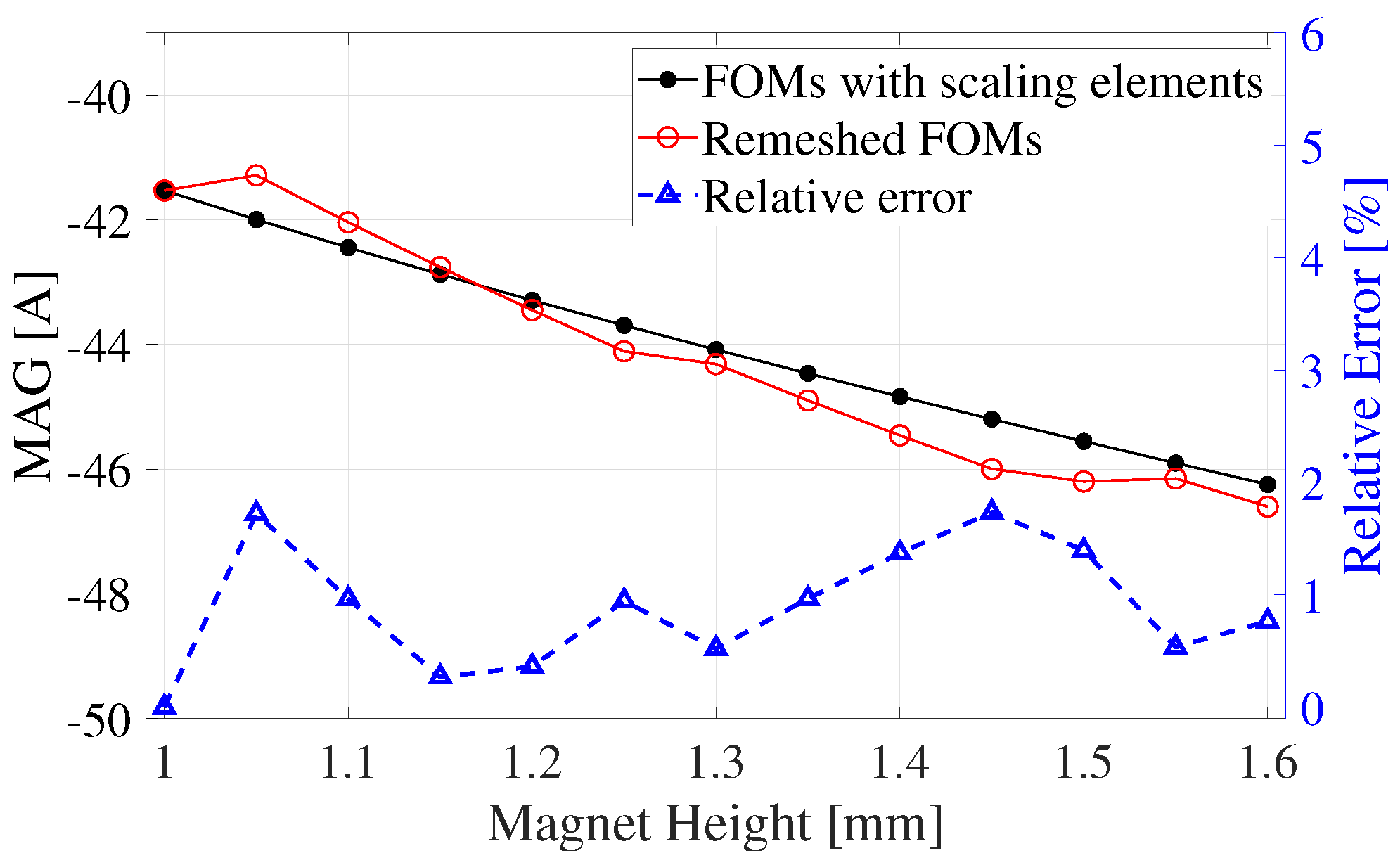
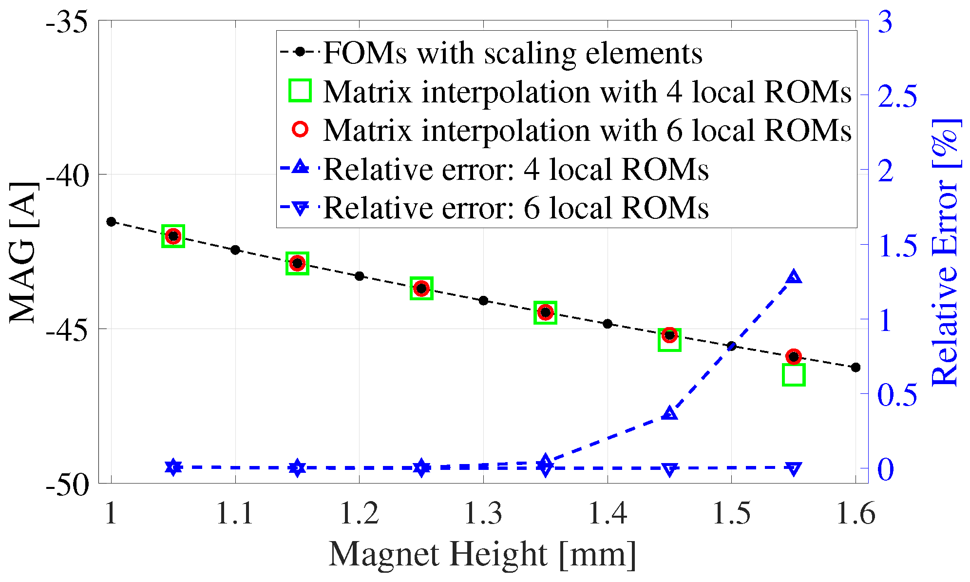
In addition, we implemented the matrix interpolation-based and algebraic parameterization-based pMOR methods to generate the geometrical parameter-independent pROMs. The position and the size of the magnet were parameterized, respectively. These two methods were first implemented on a 2D permanent magnet model to compare their computational cost and the performance of the pROMs. It was found that when sharing the same number of local ROMs and snapshot system matrices, the matrix interpolation-based pMOR method was able to generate the pROM more efficiently and the algebraic parameterization-based pMOR method gave a more accurate pROM, even in a large parameter range. Both methods were able to construct precise geometrical parameter-dependent pROMs. Then these two methods were further applied to the 3D electromagnetic energy harvester model. However, when the algebraic parameterization-based pMOR method was applied, we found that the generated reduced system matrix $K_r(\frac{1}{\alpha },\alpha )$ was singular and the pROM was unsolvable. Further research is required on this topic.

Recently, the authors in [40] suggested a new workflow for constructing a pROM of the electromagnetic system, where the position of the magnets is parameterized. Instead of scaling the elements, the model is separated into moving and non-moving parts while the mesh topology of both parts is kept constant. Future research work will evaluate and adapt this method to the electromagnetic energy harvester model.

References

1. Bai, C.; Dallasega, P.; Orzes, G.; Sarkis, J. Industry 4.0 Technologies Assessment: A Sustainability Perspective. Int. J. Prod. Econ. 2020, 229, 107776. [Google Scholar] [CrossRef]
2. Dalenogare, L.S.; Benitez, G.B.; Ayala, N.F.; Frank, A.G. The Expected Contribution of Industry 4.0 Technologies for Industrial Performance. Int. J. Prod. Econ. 2018, 204, 383–394. [Google Scholar] [CrossRef]
3. Müller, J.M.; Kiel, D.; Voigt, K. What Drives the Implementation of Industry 4.0? The Role of Opportunities and Challenges in the Context of Sustainability. Sustainability 2018, 10, 247. [Google Scholar] [CrossRef] [Green Version]
4. Hudak, N.S.; Amatucci, G.G. Small-Scale Energy Harvesting through Thermoelectric, Vibration, and Radiofrequency Power Conversion. J. Appl. Phys. 2008, 103, 101301. [Google Scholar] [CrossRef]
5. Priya, S.; Inman, D.J. (Eds.) Energy Harvesting Technologies; Springer: Boston, MA, USA, 2009. [Google Scholar]
6. Toprak, A.; Tigli, O. Piezoelectric Energy Harvesting: State-of-the-Art and Challenges. Appl. Phys. Rev. 2014, 1, 031104. [Google Scholar] [CrossRef]
7. Khan, F.U.; Qadir, M.U. State-of-the-Art in Vibration-based Electrostatic Energy Harvesting. J. Micromech. Microeng. 2016, 26, 103001. [Google Scholar] [CrossRef]
8. Tan, Y.; Dong, Y.; Wang, X. Review of MEMS Electromagnetic Vibration Energy Harvester. J. Microelectromech. Syst. 2017, 26, 1–16. [Google Scholar] [CrossRef]
9. Beeby, S.P.; Torah, R.N.; Tudor, M.J.; Glynne-Jones, P.; O’Donnell, T.; Saha, C.R.; Roy, S. A Micro Electromagnetic Generator for Vibration Energy Harvesting. J. Micromech. Microeng. 2007, 17, 1257–1265. [Google Scholar] [CrossRef]
10. Forrester, J.; Davidson, J.N.; Foster, M.P.; Stone, D.A. Circuit Simulator Compatible Model for the Ring-Dot Piezoelectric Transformer. J. Microelectromech. Syst. 2023, 32, 103–116. [Google Scholar] [CrossRef]
11. Xu, H.; Wang, Z.; Zhou, Z.; Yi, Z.; Qin, M.; Huang, Q. An Efficient Macromodel Extraction Strategy for Packaged MEMS Thermal Wind Sensor Considering Multiphysics. IEEE Sens. J. 2023, 23, 5879–5891. [Google Scholar] [CrossRef]
12. ANSYS®. Electronics Desktop, Maxwell 3D, Release 2022 R1, Maxwell Help, 19-Exporting Equivalent Circuit Data; ANSYS, Inc.: Canonsburg, PA, USA, 2022. [Google Scholar]
13. Yuan, C.; Hohlfeld, D.; Bechtold, T. Towards System-level Simulation of an Electromagnetic Energy Harvester Model via Equivalent Circuit Extraction from ANSYS Maxwell 3D. In Proceedings of the 24th International Conference on Thermal, Mechanical and Multi-Physics Simulation and Experiments in Microelectronics and Microsystems (EuroSimE), St. Julian, Malta, 24–27 April 2023. [Google Scholar]
14. Cangellaris, A.C.; Zhao, L. Model Order Reduction Techniques for Electromagnetic Macromodeling based on Finite Methods. Intern. J. Numer. Model. Electron. Netw. Devices Fields 2000, 13, 181–197. [Google Scholar] [CrossRef]
15. Zhu, Y.; Cangellaris, A.C. Finite Element-Based Model Order Reduction of Electromagnetic Devices. Intern. J. Numer. Model. Electron. Netw. Devices Fields 2002, 15, 73–92. [Google Scholar] [CrossRef]
16. Kowalski, M.E.; Jin, J.M. Model-Order Reduction of Nonlinear Models of Electromagnetic Phased-Array Hyperthermia. IEEE Trans. Biomed. Eng. 2003, 50, 1243–1254. [Google Scholar] [CrossRef]
17. Albunni, M.N.; Rischmuller, V.; Fritzsche, T.; Lohmann, B. Model-Order Reduction of Moving Nonlinear Electromagnetic Devices. IEEE Trans. Magn. 2008, 44, 1822–1829. [Google Scholar] [CrossRef] [Green Version]
18. Nicolini, J.L.; Na, D.Y.; Teixeira, F.L. Model Order Reduction of Electromagnetic Particle-in-Cell Kinetic Plasma Simulations via Proper Orthogonal Decomposition. IEEE Trans. Plasma Sci. 2019, 47, 5239–5250. [Google Scholar] [CrossRef]
19. Ahmadloo, M.; Dounavis, A. Parameterized Model Order Reduction of Electromagnetic Systems Using Multiorder Arnoldi. IEEE Trans. Adv. Packag. 2010, 33, 1012–1020. [Google Scholar] [CrossRef]
20. Panzer, H.; Mohring, J.; Eid, R.; Lohmann, B. Parametric Model Order Reduction by Matrix Interpolation. Automatisierungstechnik 2010, 58, 475–484. [Google Scholar] [CrossRef]
21. Freund, R.W. Krylov-subspace Methods for Reduced-Order Modeling in Circuit Simulation. J. Comput. Appl. Math. 2000, 123, 395–421. [Google Scholar] [CrossRef] [Green Version]
22. Moosmann, C. ParaMOR—Model Order Reduction for Parameterized MEMS Applications. Ph.D. Thesis, University of Freiburg, Freiburg, Germany, 2007. [Google Scholar]
23. Baur, U.; Benner, P.; Greiner, A.; Korvink, J.G.; Lienemann, J.; Moosmann, C. Parameter Preserving Model Order Reduction for MEMS Applications. Math. Comput. Model. Dyn. Syst. Methods Tools Appl. Eng. Relat. Sci. 2011, 17, 297–317. [Google Scholar] [CrossRef]
24. Gunupudi, P.; Nakhla, M. Multi-Dimensional Model Reduction of VLSI Interconnects. In Proceedings of the IEEE 2000 Custom Integrated Circuits Conference, Orlando, FL, USA, 24 May 2000; pp. 499–502. [Google Scholar]
25. Daniel, L.; Siong, O.C.; Chay, L.S.; Lee, K.H.; White, J. A Multiparameter Moment-Matching Model-Reduction Approach for Generating Geometrically Parameterized Interconnect Performance Models. IEEE Trans. Comput. Aided Des. Integr. Circuits Syst. 2004, 23, 678–693. [Google Scholar] [CrossRef]
26. Bechtold, T.; Hohlfeld, D.; Rudnyi, E.B. Efficient Extraction of Thin-Film Thermal Parameters from Numerical Models via Parametric Model Order Reduction. J. Micromech. Microeng. 2010, 20, 045030. [Google Scholar] [CrossRef]
27. Yuan, C.; Kreß, S.; Sadashivaiah, G.; Rudnyi, E.B.; Hohlfeld, D.; Bechtold, T. Towards Efficient Design Optimization of a Miniaturized Thermoelectric Generator for Electrically Active Implants via Model Order Reduction and Submodeling Technique. Int. J. Numer. Methods Biomed. Eng. 2020, 36, e3311. [Google Scholar] [CrossRef] [PubMed]
28. Yuan, C.; Hohlfeld, D.; Bechtold, T. Design Optimization of a Miniaturized Thermoelectric Generator via Parametric Model Order Reduction. Microelectron. Reliab. 2021, 119, 114075. [Google Scholar] [CrossRef]
29. ANSYS®. Electronics Desktop, Maxwell 3D; Release 2022 R1; ANSYS, Inc.: Canonsburg, PA, USA, 2022. [Google Scholar]
30. Whelan, P.M.; Hodgeson, M.J. Essential Principles of Physics, 2nd ed.; John Murray: London, UK, 1978. [Google Scholar]
31. ANSYS®. Electronics Desktop, Twin Builder; Release 2022 R1; ANSYS, Inc.: Canonsburg, PA, USA, 2022. [Google Scholar]
32. ANSYS®. Ansys Mechanical APDL Product; Release 2022 R1; ANSYS, Inc.: Canonsburg, PA, USA, 2022. [Google Scholar]
33. Rudnyi, E.B. System-Level Modelling of MEMS; Chapter MOR for ANSYS; Wiley VCH Verlag GmbH & Co. KGaA: Weinheim, DE, USA, 2013. [Google Scholar]
34. ANSYS®. Mechanical APDL, Release 2022 R1, Theory Reference, Chapter 5: Electromagnetics; ANSYS, Inc.: Canonsburg, PA, USA, 2022. [Google Scholar]
35. Hildebrand, F.B. Introduction to Numerical Analysis, 2nd ed.; Dover: New York, NY, USA, 1974. [Google Scholar]
36. Leon, S.J.; Björck, Å.; Gander, W. Gram-Schmidt Orthogonalization: 100 Years and More. Numer. Linear Algebra Appl. 2013, 20, 492–532. [Google Scholar] [CrossRef]
37. Amsallem, D.; Tezaur, R.; Farhat, C. Real-Time Solution of Computational Problems using Databases of Parametric Linear Reduced-Order Models with Arbitrary Underling Meshes. arXiv 2015, arXiv:1506.07153v1. [Google Scholar]
38. Roy, A.; Nabi, M. Efficient Simulation of Electro-Thermal Micro-Gripper Using pMOR. In Proceedings of the Indian Control Conference (ICC), Kanpur, India, 4–6 January 2018. [Google Scholar]
39. Roy, A.; Nabi, M.; Rahman, N. Finite Element Compatible Matrix Interpolation for Parametric Model Order Reduction of Electrothermal Microgripper. J. Comput. Des. Eng. 2021, 8, 1622–1635. [Google Scholar] [CrossRef]
40. Schütz, A.; Bechtold, T. Matrix Interpolation-based Parametric Model Order Reduction of Electromagnetic Systems with Translational Movement. In Proceedings of the 24th International Conference on Thermal, Mechanical and Multi-Physics Simulation and Experiments in Microelectronics and Microsystems (EuroSimE), Graz, Austria, 16–19 April 2023. [Google Scholar]
Figure 1. A drawing of the assembled electromagnetic energy harvester introduced in [9] (left); the schematic of the magnets and the coil (middle); cross-section through the four-magnet arrangement (right).
Electronics 12 03252 g001
Figure 2. The side view of the positions of the magnets in the z-direction with time. (left) initial resting position of the magnets; (middle) magnets at the center position; (right) magnets at the top position.
Electronics 12 03252 g002
Figure 3. Comparison of the open voltage results obtained from [9] and this work.
Electronics 12 03252 g003
Figure 4. The equivalent circuit model is constructed on the basis of the look-up table of the parametric simulation results. It is further connected to both electrical and mechanical circuits at the system level.
Electronics 12 03252 g004
Figure 5. The outer plot shows the open circuit voltage from the equivalent circuit model simulated with a simulation period of 3.5 s. The inner plot shows the voltages between 3.1 and 3.5 s.
Electronics 12 03252 g005
Figure 6. Power dissipation in the load resistor with the varying load resistance.
Electronics 12 03252 g006
Figure 7. Varying the geometrical parameter while preserving the mesh topology via scaling the elements [22].
Electronics 12 03252 g007
Figure 8. Preserve the mesh topology of the 2D permanent magnet model while changing the position of the magnet via scaling the mesh in the top and bottom air regions. An output node is selected from a fixed position in the bottom air region.
Electronics 12 03252 g008
Figure 9. Simulation results of the pROM obtained from matrix interpolation-based pMOR method. Change the position of the magnet between 0 and 1.2 mm with a step of 0.05 mm. The local ROMs are constructed at l = { 0 , 0.1 , 0.2 , , 1.2 } mm and the pROMs are interpolated at l = { 0.05 , 0.15 , 0.25 , , 1.15 } mm.
Electronics 12 03252 g009
Figure 10. Preserve the mesh topology of the 2D permanent magnet model while changing its height via scaling the mesh in the magnet and the two air regions beside the magnet. An output node is selected from a fixed position in the bottom air region.
Electronics 12 03252 g010
Figure 11. Comparison of the magnetic vector potential results between FOM and pROMs, which are obtained via matrix interpolation and algebraic parameterization-based pMOR methods, respectively.
Electronics 12 03252 g011
Figure 12. Comparison of the magnetic vector potential results between FOM and pROMs, which are obtained via matrix interpolation with three and six local ROMs, respectively.
Electronics 12 03252 g012
Figure 13. Simulation results of the pROM obtained from the algebraic parameterization-based pMOR method in a large parameter range.
Electronics 12 03252 g013
Figure 14. Simulation results from the FOM with and without scaled mesh. Scaling the elements degenerates the mesh and decreases the accuracy of the FOM.
Electronics 12 03252 g014
Figure 15. Electromagnetic energy harvester model built in ANSYS Mechanical APDL. The height of the magnets is parameterized while preserving the mesh topology via scaling the elements.
Electronics 12 03252 g015
Figure 16. Changing the height of the magnets from 1 to 1.6 mm via scaling the elements. Comparison of the results between the FOMs of the 3D electromagnetic energy harvester model with scaling elements and the remeshed FOMs.
Electronics 12 03252 g016
Figure 17. Comparison of the results between the 3D electromagnetic energy harvester FOM and the pROMs obtained via matrix interpolation-based pMOR method. The interpolated pROMs are generated on the basis of four local ROMs at {1.0, 1.1, 1.2, 1.3} mm and six local ROMs at {1.0, 1.1, 1.2, 1.3, 1.4, 1.5, 1.6} mm, respectively.
Electronics 12 03252 g017