1. Introduction
Considerable research has been conducted on autonomous vehicle systems for self-driving cars. One key component of self-driving cars is an understanding of human driving behavior to avoid human–machine conflict [
1,
2,
3,
4]. Driving behavior analysis has become crucial for traffic safety. With recent advances in machine learning techniques [
3,
4], data-driven approaches to complicated human behavior modeling have become increasingly feasible. In particular, several studies have made significant progress using deep learning techniques.
Among recent learning approaches [
3,
4], in addition issues regarding the design of network structures, another critical issue has been the collection of large amounts of training data. With the popularization of dash cams, the driving data provided cannot meet the needs of driving behavior analysis. More abundant driving data are needed to analyze driving behavior more comprehensively and thus improve traffic safety. Autonomous vehicle systems typically collect data from onboard sensors and extract information for specific analyses [
1]. These may encompass images captured by in-car cameras and proprioceptive driving data recorded by onboard diagnostic systems. The extraction of adequate data segments for neural network training and testing is critical. For instance, learning road sign recognition requires certain traffic scene images or modeling a driver’s acceleration behavior using selected gas pedal information. Large training datasets are typically used in deep neural networks to achieve better performance.
Conventionally, data annotation or labeling has been mainly completed manually and sometimes through crowdsourcing. For driving data, a dataset collected according to different tasks will contain various scenes and features. The selection and filtering of adequate data require significant time and human labor. The development of technologies for searching specific traffic scenes within a large number of image sequences has become important. The main goals of this paper are to propose an image data extraction system based on geographic information and driving behavior analysis using various types of driving data. We used information derived from a geographic information system (GIS) and a global positioning system (GPS) along with recorded driving videos to identify road scenes with static objects such as traffic lights, traffic signs, bridges, and tunnels. Additionally, we utilized an onboard diagnostic II (OBD-II) and a controller area network bus (CANbus) logger to collect driving data [
5]. By measuring several parameters at a high sampling rate, we can completely observe driving behaviors and understand the influences of traffic and road infrastructure.
To analyze the relationship between driving behavior and transportation infrastructure, visualization on a map provides a means of better observation and investigation. We used machine learning methods to extract unique features from the driving data and then mapped these features to the RGB color space to visualize the driving behavior. Data mining algorithms [
6] were utilized for data analysis and to classify driving behavior into four categories, ranging from normal to aggressive. A regression analysis [
7] was then conducted on the relationship between aggressive driving behavior and road features at intersections. Several traffic improvements were proposed for specific intersections and roads to make drivers and pedestrians safer.
The contributions of this paper are as follows. (a) We present a road scene extraction approach for specific landmarks and transportation infrastructure indicators. (b) To perform a more comprehensive analysis, we present visual driving behavior, aggressive driving behavior, and traffic light information on a map to associate driving behavior with roads. (c) Based on the results of the driving behavior analysis, suggestions and verifications for traffic improvement at intersections are presented, with their intention being to prevent accidents.
2. Related Works
2.1. Data Extraction
As learning-based algorithms [
3,
4] become popular, the acquisition of training and testing data has become crucial. For unsupervised classification, Hornauer et al. and Wu et al. [
8,
9] proposed unsupervised image classification methods for extracting images similar to those provided by general users [
10]. However, good training data should be reflected consistently in the testing data. For supervised classification [
1,
2], the data were manually labeled. People need to have a similar understanding to annotate the same scene. The network of this approach is based on feature similarity for a first-person driving image query. However, this may not fully meet the needs of the users.
In addition, Naito et al. [
11] proposed a browsing and retrieval approach to driving data. Their approach provides a multidata browser, a retrieval function based on queries and similarities, and a quick browsing function to skip extra scenes. The top-
N images that were highly similar to the current driving scenario were retrieved from a database for scene retrieval. While an image sequence is processed, this approach calculates the similarity between the input scene and the scenes stored in the database. A predefined threshold was used to identify similarities between the images. Because the approach mainly searched for the driving video itself, it could not be determined whether the images contained objects or information that was interesting to the users for precise extraction.
2.2. Driving Behavior Analysis
The key technologies for automotive driving-assistance systems have matured [
12]. However, autonomous vehicles can still not be employed without human drivers. Owing to the current limitations of driving-assistance systems, researchers and developers are seeking solutions to improve human driving capabilities. Because changing driving habits is challenging, developing a human-centered driving environment to avoid dangerous situations is crucial. By understanding the relationships between traffic lights, road infrastructure, and driving behavior, suggestions for transportation improvement can be provided. In addition, understanding human reactions is also a crucial issue for mixing human-driven and self-driving cars.
Regarding driving behavior analysis, Liu et al. [
13,
14] proposed a method that uses various types of sensors connected to a control area network. A deep sparse autoencoder (SAE) was then used to extract hidden features from the driving data to visualize driving behavior. Constantinescu et al. [
15] used both principal component analysis (PCA) and hierarchical cluster analysis (HCA) techniques to analyze driving data. The performance of their techniques was verified by classifying the driving behavior into six categories based on aggressiveness. In the approach proposed by Kharrazi et al. [
16], driving behavior was classified into three categories—calm, normal, and aggressive—using quartiles and
K-means clustering. Their results demonstrated that
K-means clustering can provide good classification results for driving behaviors.
To analyze the correlation between driving and road facilities, Tay et al. [
17] used a regression model to associate driving accidents with environmental factors. Drivers were liable to run when driving accidents occurred at night, on a bridge, and so on. Wong et al. [
7] utilized negative binomial regression to analyze the number of driving accidents and road features at intersections. Road intersections can also be improved using simulations based on the analysis results. Schorr et al. [
18] presented an approach for recording driving data in one- and two-way lanes. Based on an analysis of variance (ANOVA), a conclusion regarding the impact of lane width on driving behavior was drawn. Abojaradeh et al. [
19] proposed a method for identifying driving behaviors and driver mistakes based on questionnaires and highlighted their effects on traffic safety. They used regression analysis to derive the correlation between the number of accidents and types of dangerous driving behaviors.
Regarding the improvement of transportation infrastructure, various suggestions have been proposed for different road and intersection designs. Chunhui et al. [
20] proposed an approach to optimizing signal lights at intersections to make pedestrian crossing easier [
21]. The efficiency of intersections was improved by reducing the frequency of conflicts between turning vehicles and pedestrians. Ma et al. [
22] proposed a technique for adding a dedicated left-turn lane and waiting area based on the average daily traffic volume at an intersection. The proposed method can facilitate more vehicles waiting to make a left turn. They also analyzed three common left-turn operation scenarios at intersections and compared the differences between them. In addition to suggestions for road infrastructure, several traffic improvements have been suggested based on traffic light analysis. Anjana et al. [
23] presented a method based on different traffic volumes at intersections to evaluate the safety of green traffic lights. The results showed that exclusive left-turn lanes and countdown timers can improve traffic safety at intersections.
3. Image Data Extraction
OpenStreetMap (OSM) [
14] is an open and global map that allows everyone to freely build map content. The geographic information system in transportation (GIS-T) [
24] is an open transportation map data storage system used in Taiwan. The maps of GIS-T are mainly divided into four categories, including basic geographic maps, transportation systems, sightseeing information, and disaster prevention information.
To enact the proposed approach, we first collected information regarding traffic lights, traffic signs, and road information from OSM and GIS-T. Traffic and road information were used to identify locations of interest using GPS coordinates. We compared the GPS information obtained from the driving data to the locations of interest. The associated images were then extracted and stored in video sequences for specific applications, such as training and testing data for traffic light detection.
Figure 1 illustrates a flowchart of image data extraction.
The driving recorder contained images at a resolution of 1280 × 720 and with a 110° field of view (FOV) in the horizontal direction. To extract suitable image data, users must consider the geographic range of the target. For example, in road scene extraction with traffic lights, the size of the traffic signal in an image may be larger than 25 × 25 pixels for specific tasks. This corresponds to approximately 50 m away from the vehicle; thus, the video should be rewound by 5 s before starting image data extraction.
We established an interface for user operations. The interface structure is divided into two parts: image extraction and video filtering. The items included in the image data extraction were traffic lights and traffic signs, whereas the video filtering included highways and tunnels. A program interface was created for users to easily use the data and assign parameters. It consists of a folder for selection, an item menu for extraction, an OSM map display, and a driving image screen. The user first selects the folder where the driving record video and driving GPS information are located, and the folder where the extracted image will be stored. The user then selects traffic infrastructure or road information for extraction. At the interface, the vehicle’s GPS trajectory and user-selected traffic infrastructure simultaneously overlay the OSM window, and a synchronized driving video is displayed on the right for inspection.
4. Driving Behavior Analysis
To demonstrate the proposed approach, we analyzed driving behavior and its correlation with traffic and road features. Driving behavior was classified as normal or aggressive and analyzed through data visualization and a regression model of the number of aggressive driving behaviors and road features.
A flowchart of the driving behavior analysis is presented in
Figure 2. First, we used the ODB-II and CANbus loggers to collect driver data. We then utilized an SAE to extract features from the driving data and compress the high-dimensional features into three dimensions. Subsequently, we mapped the three-dimensional features to the RGB space for display on the OSM. Moreover, we used the
K-means clustering algorithm to further classify the driving behavior based on aggressiveness. Finally, we used a negative binomial regression model to analyze the road features at intersections and interchanges.
4.1. Data Collection
In addition to exteroceptive sensors (such as LiDAR, GPS, and cameras), the information collected via the proprioceptive sensors of the vehicle can also be used to analyze driving behavior [
5,
25]. Sensor data derived directly from vehicle operations can provide more comprehensive driving information.
An OBD system is an automotive electronic system installed in a vehicle to monitor the vehicle’s operating status and report abnormal signals. An OBD-II system is a vehicle diagnostic system that contains more comprehensive diagnostic trouble codes and emissions control. A CANbus is a network characterized by its ability to allow multiple microcontrollers or devices on the network to communicate directly with each other without the need for a host to control communication on the network. The CANbus is a protocol supported by OBD-II. A CANbus logger is a recorder for a CANbus system. We used ODB-II and CANbus loggers for driver data collection. Unlike the information obtained from GPS receivers (including GPS messages, vehicle speed, and acceleration), which most previous studies were limited to, the data obtained through OBD-II and CANbus loggers can include various types of driving data for analysis. The specific data types used for the proposed driving behavior analysis are as follows.
OBD-II: engine rotation speed, engine load, throttle pedal position, acceleration XYZ, and vehicle speed.
CANbus logger: engine rotation speed, throttle pedal position, braking pedal position, steering angle, wheel speed, and vehicle speed.
GPS receiver: GPS and coordinated universal time (UTC).
Moreover, the DDD17 dataset [
26] has 12 h of recorded data using a dynamic and active-pixel vision sensor (DAVIS). It is the first open dataset of annotated DAVIS driving records. The driving data recorded include steering angle, speed, GPS, accelerator position, and so on. In addition, the driving data were collected under different conditions for six days and over 1000 km of different roads. We selected the same driving data categories as we collected with the CANbus loggers for analysis, including vehicle speed, steering wheel steering angle, engine speed, engine torque, accelerator and brake position, and acceleration. The UAH DriveSet [
27] dataset is a public collection of data obtained via the driving monitoring application DriveSafe [
28], which captures data using the sensors of a mobile phone. The driving data were collected by six different drivers and vehicles performing three different driving behaviors (normal, drowsy, and aggressive) on two types of roads (motorway and secondary road). This dataset contains more than 500 min of natural driving and related raw data. We used normal and aggressive driving data from this dataset to verify whether the proposed approach can effectively classify aggressive driving behaviors. These two datasets are commonly used datasets for driver behavior analysis. There are some biases or limitations inherent in these two datasets because of sample selections and sensor problems.
4.2. Visualization of Driving Behavior
The relationship between driving behavior and traffic infrastructure can be observed through data visualization on a map. An autoencoder (AE) is a neural network for the unsupervised learning efficient coding of unlabeled data. An SAE is an improved version of an AE. Using an SAE does not requires that driving data be manually labelled and can generate similar data through learning for feature extraction. We used the SAE to extract features from the driving data, compress the high-dimensional features into three dimensions, and map the 3D features onto RGB space for display on the OSM. The loss function with sparse constraints is given as follows:
where
J(
W,
b) is the cost function with parameters
W and
b. The parameter
β controlling the weight of the sparsity penalty term.
ρ is a sparsity parameter, and
is the average activation of hidden unit
j. Moreover,
s2 is the number of neurons in the hidden layer, and
is Kullback–Leibler divergence between
ρ and
.
Unlike an autoencoder (AE), an SAE has a penalty term added to the loss function. Thus, the activation of hidden nodes decreases to the required value. Using this property, the relative entropy is added to the loss function to penalize the value of the average activation degree being far away from the level ρ. The parameters maintain the average degree of activation of the hidden nodes at this level. Thus, the loss function only requires the addition of a penalty term for relative entropy without sparse constraints.
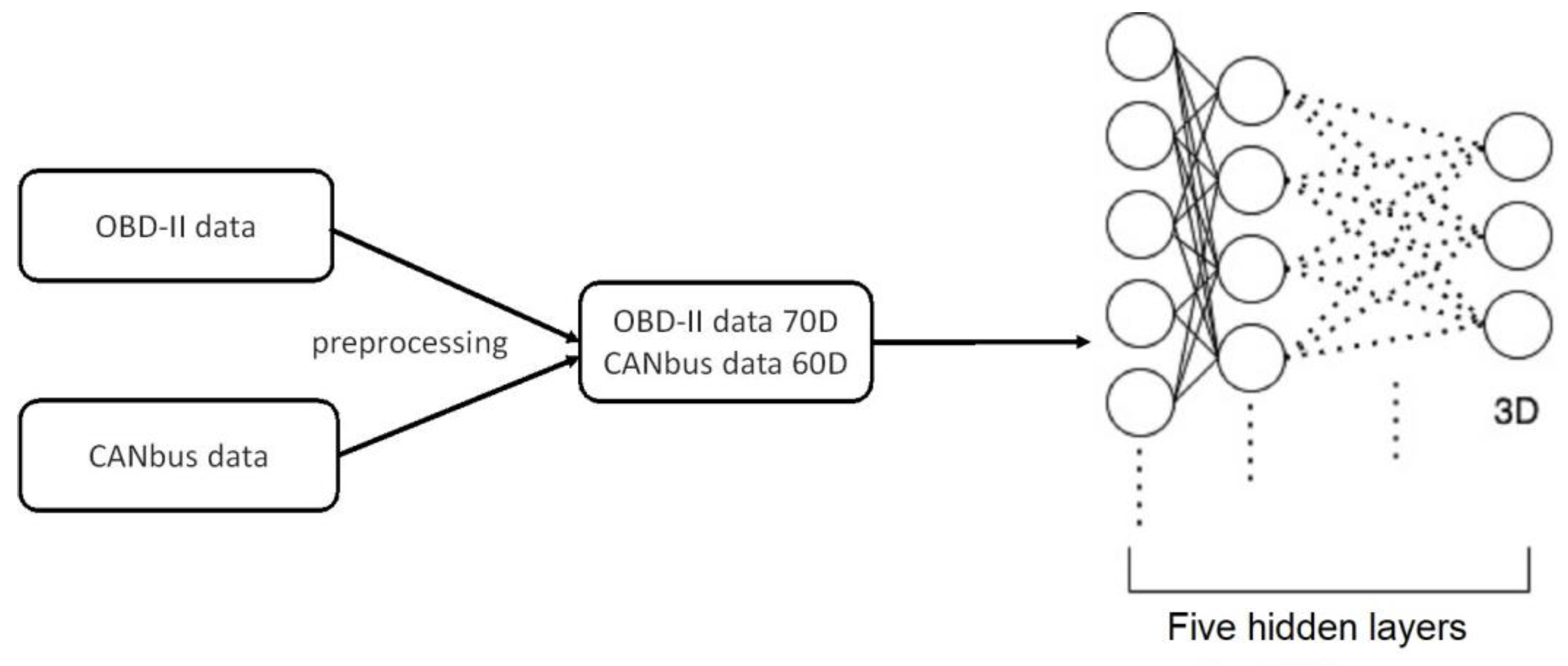
Figure 3 illustrates the flowchart and network structure used to visualize driving behavior. The network contained nine hidden layers, and the dimensionality reduction of each layer was half the number of nodes in the previous layer. The data collected by OBD-II contained seven types and 70 dimensions after the windowing process. Thus, the dimension reduction in the network is 70 → 35 → 17 → 8 → 3 → 8 → 17 → 35 → 70, and the features are extracted by the last five layers. The data collected by the CANbus logger contained six types and 60 dimensions after the windowing process. Likewise, the input to the network comprises 60 nodes, and the dimension reduction is given as follows: 60 → 30 → 15 → 7 → 3 → 7 → 15 → 30 → 60. Finally, driving behavior was visualized using the OSM.
Figure 4 shows an example of the driving behavior visualized on the OSM for the network structure 70 → 35 → 17 → 8 → 3 → 8 → 17 → 35 → 70.
K-means clustering [
6] is a clustering algorithm mainly used in data mining. The purpose of
K-means is to divide
n data points into
k clusters so that each data point is classified into the category corresponding to the nearest cluster center. The elbow method [
6] is a technique used to find the number of clusters for
K-means clustering. In the proposed approach, we used the
K-means clustering algorithm to further classify driving behavior. The elbow method was used to determine the most appropriate
k value to classify driving behavior according to aggressiveness. Based on the results of the elbow method, the error values did not change significantly after
K was set to four. Thus, the inflection point of the error curve was the position of
K = 4. Driving behavior is classified according to four levels, ranging from normal to aggressive, and the most aggressive driving behavior is marked on the OSM.
4.3. Negative Binomial Regression
The negative binomial regression model [
7] is a well-known technique used to model over-dispersed data. It is an extended version of the Poisson regression to process the data overdispersion problem. In the proposed approach, a negative binomial regression analysis was conducted to relate the number of aggressive driving behaviors (the dependent variable) to various independent variables to capture the road features at intersections and interchanges. The negative binomial regression model is used to predict the number of aggressive driving behaviors
, defined as
where
βi is the correlation term associated with each road feature vector
xki and
is an error term. Pearson’s chi-squared test was performed [
29] to verify whether the data were overdispersed. When the ratio was greater than one, the data were considered overdispersed.
To evaluate whether negative binomial regression could better fit our data, the Akaike information criterion (AIC) was computed for these two models [
30]. The AIC is an effective measure of data fitting in regression models and is defined as
where
k is the number of features, and ln(
L) is the maximum likelihood. A smaller
AIC value implies a better-fitting model.
After classifying driving behavior using
K-means clustering, aggressive driving behavior was found to occur more frequently at interchanges and intersections. Negative binomial regression analysis was performed for these two specific driving scenarios. We adopted the road features proposed by Wong [
16] and those commonly appearing in Taiwanese road scenes.
Interchanges: (1) section length, (2) lane width, (3) speed limit, and (4) traffic flow.
Four-arm intersection: (1) no lane markings, (2) straight-lane markings, (3) left-lane markings, (4) right-lane markings, (5) shared-lane markings, (6) shared-lane markings at the roadside, (7) motorcycle priority, and (8) branch road.
Three-arm intersection: (1) no lane markings, (2) straight-lane markings, (3) shared-lane markings at the roadside, (4) lane ratio, (5) motorcycle priority, and (6) branch road.
5. Experimental Results and Discussion
We divided the experiments into two parts: the image data extraction of training and testing datasets and the driving behavior analysis based on the driving and road features.
5.1. Extraction of Training and Testing Data
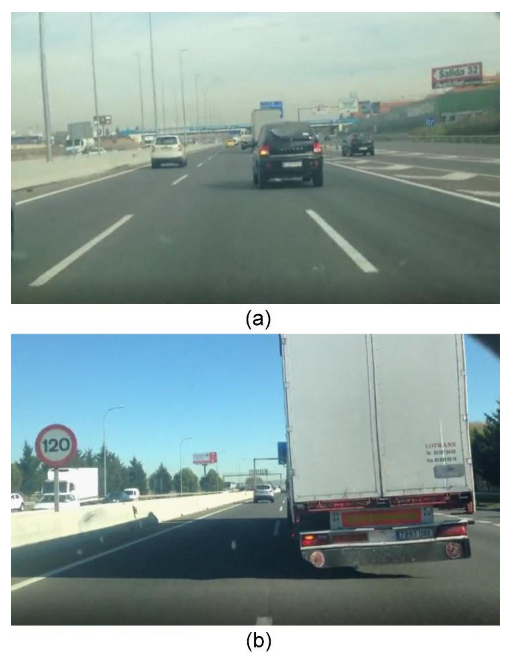
We demonstrate the image data extraction for road scenes with traffic lights.
Figure 5a shows the driving trajectory (indicated by the red curve) and traffic light positions (indicated by blue circles) on the OSM. The driving videos were filtered through an extraction system to contain traffic lights from far to near. The extracted images in
Figure 5b,c correspond to orange dots (a) and (b) in
Figure 5a, respectively.
5.2. Driving Behavior Analysis
For the driving behavior analysis, we first presented the visualization and K-means classification and then performed an analysis of the driving behavior and road features.
5.2.1. Visualization and K-Means Classification
We used five segments of driving data from the UAH DriveSet, in which the drivers showed normal and aggressive behaviors separately. In each data segment, 50 samples were used for classification. The results are presented in
Table 1 with the percentage of correct classifications, where D1–D5 represent the five drivers.
N and
A denote normal and aggressive driving, respectively. The table shows that
K-means classification can provide satisfactory classification results for normal and aggressive driving behaviors.
Figure 6 shows the visualized driving behavior and the corresponding driving data chart.
Figure 6a shows the visualized driving behavior (including aggressive driving), using the driving data in the UAH DriveSet visualized on the OSM with traffic light location information. The red circles A and B in
Figure 6a correspond to the driving data chart enclosed by the red rectangles A and B, respectively, in
Figure 6b. The driving images corresponding to the red circles A and B in
Figure 6a are shown in
Figure 7a,b, respectively. In this example, the aggressive driving behavior at the location indicated by red circle A in
Figure 6a was due to sudden braking caused by the car in front at the intersection (
Figure 7a), and that at the location indicated by red circle B in
Figure 6b was due to the driver changing lanes (
Figure 7b).
By visualizing the driving behavior and displaying aggressive driving behaviors on OSM with reference to the driving video, we can observe a correlation between driving behavior and traffic infrastructure. The three situations were analyzed as follows:
- a.
Influence of two-way lanes on driving behavior: The vehicle speed in a two-way lane was higher than that in a one-way lane. Thus, aggressive driving behaviors with fast driving and emergency braking are more likely to occur in two-way lanes.
- b.
Influence of traffic lights on driving behavior: The most aggressive driving behavior occurs at intersections. There may be many reasons for this, such as fast-changing signals and poor road design. This generally causes more conflicts between drivers and other vehicles.
- c.
Influence of interchanges on driving behavior: In highway traffic, the most aggressive driving behaviors occur at interchanges. A vehicle entering an interchange entrance tends to drive in the inner lane. This generally causes the other drivers to change lanes or slow down.
5.2.2. Negative Binomial Regression
Because aggressive driving behaviors frequently occur near intersections and interchanges, we further investigated these driving scenarios using negative binomial regression analysis of the correlation between the number of aggressive behaviors and road features.
The
p-value can be used to evaluate the statistical significance of the features of aggressive driving behaviors [
31]. The following two driving scenarios were examined.
Four-Arm Intersection: Eight different road features were defined at the intersections. The regression analysis is shown in
Figure 8a, where Intercept is the error term of the regression model, LEFT is the left-turn lane mark, STRA is the straight lane mark, RIGHT is the right-turn lane mark, TWO is the shared lane mark, SHARE is the shared lane mark on the side of the road, NO is no lane mark, MOTOR is the number of priority locomotive lanes, CROSS is the number of branch roads, and the coefficient term is the parameter of the regression model. The features that have considerable impacts on aggressive driving behaviors included “straight lane marking,” “shared lane marking at roadside,” and “no lane marking.” The influences of these features on the driving behavior demonstrated positive, negative, and positive correlations, respectively. When “
p > |
z|” < 0.05 held, the feature significantly affected aggressive behavior.
Highway Interchange: Four different road features were defined for highways. The regression analysis results are shown in
Figure 8b, where LONG is the length of interchange, LANE is the lane width, LIMIT is the ramp speed limit, and FLOW is the average daily traffic volume. The features that had a considerable impact on aggressive driving behaviors were “speed limit” and “length of interchange.” The influences of these features on driving behavior showed positive and negative correlations, respectively.
5.3. Discussion
Our approach is mainly divided into two parts: image data extraction and driving behavior analysis. For the first part, we used open-source traffic and road map data as a database. We compared it with the driving video and GPS information imported by the user and used extracted images containing the items required by the user as a data set. According to a previous method proposed by Naito et al. [
11], the method mainly searched for the driving video itself. It could not be determined whether the images contained objects or information that was interesting to the users for precise extraction.
The second part involved the analysis of driving behavior. We first used OBD-II and CANbus loggers to obtain driving data. Unlike the information obtained from GPS receivers (with GPS messages, vehicle speed, and acceleration), which previous methods were limited to, the data obtained through OBD-II and CANbus loggers can include various types of driving data to analyze in more details. The data collected via OBD-II were comprised of seven types and the data collected by the CANbus logger were comprised of six types. However, it might be difficult to collect data for some older vehicles. Moreover, for data preprocessing, we first needed to find the maximum and minimum values of the data and then scaled the data values into [−1, 1]. Since each driving feature is independent, different features must be treated separately when doing scaling. The analysis results could be biased due to sample selections and sensor problems.
We then used the SAE for feature extraction and
K-means to identify normal and aggressive driving behaviors to observe the relationship between the driver and the driving environment. We also used UAH DriveSet and driving videos to verify that our approach can indeed find aggressive driving behaviors and specific driving events across a large volume of driving data. After that, a negative binomial regression analysis was performed for specific scenarios. Through the analysis results, lane ratios, no lane markings, and straight lane markings were found to be important features that affect aggressive driving behavior. Finally, we conducted a case analysis of a single intersection. For the previous method proposed by Liu et al. [
13], various types of sensors connected to a control area network for driving behavior analysis were used. Although this approach can present driving behavior in a driving color map, it cannot observe more associations between driving behavior and roads or other facilities.
Several evaluation metrics can be used to measure the performance of a classifier. Different applications have different goals for specific evaluation metrics. For the proposed approach, we used K-means classification to perform binary classification of normal and aggressive driving behaviors. The most important metric is the accuracy rate, and the significance of other evaluation metrics is relatively limited. Therefore, the results are presented with the percentage of correct classifications, and K-means classification can provide satisfactory classification results.
Traffic improvement suggestions and verification were proposed based on the analysis of a case study at an intersection. This needs to be verified to prove that the proposal is effective in reducing aggressive driving behavior. We found intersections with features similar to the proposed improvements among the existing intersections and collected driving data and driving videos for verification. The results showed that several traffic problems are significantly improved. No conflicts between the driving of vehicles and the passing of pedestrians exist.
6. Conclusions
We have presented an approach to image data extraction and driving behavior analysis using geographic information and driving data. We used information derived from geographic and global positioning systems for image data extraction. Moreover, we used OBD-II and CANbus loggers to record various types of driving data for driving behavior analysis. We used data mining algorithms for data analysis and to classify driving behavior into four categories, ranging from normal to aggressive. We conducted a regression analysis on the relationship between aggressive driving behavior and road features at intersections. The results showed that lane ratios, no lane markings, and straight lane markings are important features that affect aggressive driving behaviors. Finally, traffic improvements were proposed based on the analysis of a case study at an intersection.
In the future, we will add more, different extraction items for data sets and more, different drivers and vehicles for a more accurate analysis of driving behavior. Moreover, for the regression analysis, if more samples are used, the accuracy will be higher. However, there is no certain approach to determining the adequate sample size. In the proposed approach, we can obtain good results with at least 20 observations. We will add more observations for the regression analysis to obtain more accurate results.
Author Contributions
Methodology, J.-Z.Z. and H.-Y.L.; supervision, H.-Y.L. and C.-C.C.; writing—original draft, J.-Z.Z.; writing—review and editing, H.-Y.L. and C.-C.C. All authors have read and agreed to the published version of the manuscript.
Funding
This work was partially financially supported by Create Electronic Optical Co., LTD, Taiwan. The authors would like to thank the Ministry of Science and Technology of Taiwan for financially supporting this research under Contract No. MOST 111-2221-E-239-027.
Data Availability Statement
Not applicable.
Conflicts of Interest
The authors declare no conflict of interest.
References
- Dong, B.T.; Lin, H.Y. An on-board monitoring system for driving fatigue and distraction detection. In Proceedings of the 2021 IEEE International Conference on Industrial Technology (ICIT 2021), Valencia, Spain, 10–12 March 2021. [Google Scholar]
- Wawage, P.; Deshpande, Y. Smartphone sensor dataset for driver behavior analysis. Data Brief 2022, 41, 107992. [Google Scholar] [CrossRef] [PubMed]
- Zhang, J.Z.; Lin, H.Y. Driving behavior analysis and traffic improvement using onboard sensor data and geographic information. In Proceedings of the 7th International Conference on Vehicle Technology and Intelligent Transport Systems (VEHITS 2021), Prague, Czech Republic, 28–30 April 2021; pp. 284–291. [Google Scholar]
- Hartford, J.S.; Wright, J.R.; Leyton-Brown, K. Deep learning for predicting human strategic behavior. In Proceedings of the 30th Conference on Neural Information Processing Systems (NIPS 2016), Barcelona, Spain, 5–10 December 2016. [Google Scholar]
- Malekian, R.; Moloisane, N.R.; Nair, L.; Maharaj, B.; Chude-Okonkwo, U.A. Design and implementation of a wireless OBD II fleet management system. IEEE Sens. J. 2014, 13, 1154–1164. [Google Scholar] [CrossRef]
- Thorndike, R.L. Who belongs in the family? Psychometrika 1953, 18, 267–276. [Google Scholar] [CrossRef]
- Wong, C.K. Designs for safer signal-controlled intersections by statistical analysis of accident data at accident blacksites. IEEE Access 2019, 7, 111302–111314. [Google Scholar] [CrossRef]
- Hornauer, S.; Yellapragada, B.; Ranjbar, A.; Yu, S. Driving scene retrieval by example from large-scale data. In Proceedings of the IEEE/CVF Conference on Computer Vision and Pattern Recognition (CVPR) Workshops, Long Beach, CA, USA, 15–20 June 2019; pp. 25–28. [Google Scholar]
- Wu, Z.; Xiong, Y.; Yu, S.X.; Lin, D. Unsupervised feature learning via non-parametric instance discrimination. In Proceedings of the 2018 IEEE/CVF Conference on Computer Vision and Pattern Recognition, Salt Lake City, UT, USA, 18–23 June 2018; pp. 3733–3742. [Google Scholar]
- Wu, Z.; Efros, A.A.; Yu, S.X. Improving generalization via scalable neighborhood component analysis. In Proceedings of the European Conference on Computer Vision (ECCV), Munich, Germany, 8–14 September 2018; pp. 685–701. [Google Scholar]
- Naito, M.; Miyajima, C.; Nishino, T.; Kitaoka, N.; Takeda, K. A browsing and retrieval system for driving data. In Proceedings of the 2010 IEEE Intelligent Vehicles Symposium (IVS), La Jolla, CA, USA, 21–24 June 2010; pp. 1159–1165. [Google Scholar]
- Lin, H.Y.; Dai, J.M.; Wu, L.T.; Chen, L.Q. A vision based driver assistance system with forward collision and overtaking detection. Sensors 2020, 20, 5139. [Google Scholar] [CrossRef]
- Liu, H.; Taniguchi, T.; Takano, T.; Tanaka, Y.; Takenaka, K.; Bando, T. Visualization of driving behavior using deep sparse autoencoder. In Proceedings of the 2014 IEEE Intelligent Vehicles Symposium (IVS), Dearborn, MI, USA, 8–11 June 2014; pp. 1427–1434. [Google Scholar]
- Liu, H.; Taniguchi, T.; Tanaka, Y.; Takenaka, K.; Bando, T. Visualization of driving behavior based on hidden feature extraction by using deep learning. IEEE Trans. Intell. Transp. Syst. 2017, 18, 2477–2489. [Google Scholar] [CrossRef]
- Constantinescu, Z.; Marinoiu, C.; Vladoiu, M. Driving style analysis using data mining techniques. Int. J. Comput. Commun. Control. 2010, 5, 654–663. [Google Scholar] [CrossRef]
- Kharrazi, S.; Frisk, E.; Nielsen, L. Driving behavior categorization and models for generation of mission-based driving cycles. In Proceedings of the IEEE Intelligent Transportation Systems Conference 2019, Auckland, New Zealand, 27–30 October 2019; pp. 1349–1354. [Google Scholar]
- Tay, R.; Rifaat, S.M.; Chin, H.C. A logistic model of the effects of roadway, environmental, vehicle, crash and driver characteristics on hit-and-run crashes. Accid. Anal. Prev. 2008, 40, 1330–1336. [Google Scholar] [CrossRef] [PubMed]
- Schorr, J.; Hamdar, S.H.; Silverstein, C. Measuring the safety impact of road infrastructure systems on driver behavior: Vehicle instrumentation and exploratory analysis. J. Intell. Transp. Syst. 2016, 21, 364–374. [Google Scholar] [CrossRef]
- Abojaradeh, M.; Jrew, B.; Al-Ababsah, H. The effect of driver behavior mistakes on traffic safety. Civ. Environ. Res. 2014, 6, 39–54. [Google Scholar]
- Chunhui, Y.; Wanjing, M.; Ke, H.; Xiaoguang, Y. Optimization of vehicle and pedestrian signals at isolated intersections. Transp. Res. Part B Methodol. 2017, 98, 135–153. [Google Scholar]
- Wang, Y.; Qian, C.; Liu, D.; Hua, J. Research on pedestrian traffic safety improvement methods at typical intersection. In Proceedings of the 2019 4th International Conference on Electromechanical Control Technology and Transportation (ICECTT), Guilin, China, 26–28 April 2019; pp. 190–193. [Google Scholar]
- Ma, W.; Liu, Y.; Zhao, J.; Wu, N. Increasing the capacity of signalized intersections with left-turn waiting areas. Transp. Res. Part A Policy Pract. 2017, 105, 181–196. [Google Scholar] [CrossRef]
- Anjana, S.; Anjaneyulu, M. Safety analysis of urban signalized intersections under mixed traffic. J. Saf. Res. 2015, 52, 9–14. [Google Scholar]
- GIS-T. Available online: https://gist.motc.gov.tw/ (accessed on 25 January 2020).
- Yeh, T.W.; Lin, S.Y.; Lin, H.Y.; Chan, S.W.; Lin, C.T.; Lin, Y.Y. Traffic light detection using convolutional neural networks and lidar data. In Proceedings of the 2019 International Symposium on Intelligent Signal Processing and Communication Systems (ISPACS), Taipei, Taiwan, 3–6 December 2019; pp. 1–2. [Google Scholar]
- Binas, J.; Neil, D.; Liu, S.C.; Delbruck, T. Ddd17: End-to-end davis driving dataset. In Proceedings of the 2017 Workshop on Machine Learning for Autonomous Vehicles, Sydney, Australia, 6–11 August 2017; pp. 1–9. [Google Scholar]
- Romera, E.; Bergasa, L.M.; Arroyo, R. Need data for driver behaviour analysis? Presenting the public uah-driveset. In Proceedings of the 2016 IEEE 19th International Conference on Intelligent Transportation Systems (ITSC), Rio de Janeiro, Brazil, 1–4 November 2016; pp. 387–392. [Google Scholar]
- Bergasa, L.M.; Almería, D.; Almazán, J.; Yebes, J.J.; Arroyo, R. Drivesafe: An app for alerting inattentive drivers and scoring driving behaviors. In Proceedings of the IEEE Intelligent Vehicles Symposium (IVS), Dearborn, MI, USA, 8–11 June 2014; pp. 240–245. [Google Scholar]
- Pearson, K. X. on the criterion that a given system of deviations from the probable in the case of a correlated system of variables is such that it can be reasonably supposed to have arisen from random sampling. Lond. Edinb. Dublin Philos. Mag. J. Sci. 1900, 50, 157–175. [Google Scholar] [CrossRef]
- Akaike, H. A new look at the statistical model identification. IEEE Trans. Autom. Control. 1974, 19, 716–723. [Google Scholar] [CrossRef]
- Dahiru, T. P-value, a true test of statistical significance? A cautionary note. Ann. Ib. Postgrad. Med. 2008, 6, 21–26. [Google Scholar] [CrossRef] [PubMed]
| Disclaimer/Publisher’s Note: The statements, opinions and data contained in all publications are solely those of the individual author(s) and contributor(s) and not of MDPI and/or the editor(s). MDPI and/or the editor(s) disclaim responsibility for any injury to people or property resulting from any ideas, methods, instructions or products referred to in the content. |
© 2023 by the authors. Licensee MDPI, Basel, Switzerland. This article is an open access article distributed under the terms and conditions of the Creative Commons Attribution (CC BY) license (https://creativecommons.org/licenses/by/4.0/).


