Passive Direct Position Determination Based on KL Transform and Feature Matching

Abstract

In this article, the problem of simultaneously estimating and localizing multiple-input multiple-output (MIMO) radar emitters is considered for a distributed multi-station passive localization system, wherein the transmitted signal is unknown for receiver stations. To achieve highly accurate and robust localization performance, a novel algorithm based on the direct position determination (DPD) algorithm, Karhunen–Loève (KL) transform, and feature matching (FM) is addressed to jointly estimate the emitter position and the unknown signal waveform. First, we further derive the objective function of the DPD method and present an enhanced strategy to exploit as much waveform information as possible without any prior knowledge. By applying KL transform and FM techniques, the proposed method achieves MIMO radar emitter identification and emitter localization. The numerical results show that the proposed algorithm outperforms the existing DPD approaches which ignore the transmitted signals, especially for a low signal-to-noise ratio (SNR).

1. Introduction

Distributed multi-station passive localization (DMPL) has been widely researched due to its advantages of flexible system configuration, high-degree-of-freedom signal processing mechanism, and high accuracy [1,2,3,4,5]. As a high-performance localization technique, the application of DMPL is closely related to the emitter signal model, type of interference, and application scenarios. Most of the existing passive localization and localization technologies neglect the processing of the waveform information of the emitter signal, and also lack focusing on the localization of the radiation source of a novel radar system. The MIMO radar, as one of the representatives of the novel radar system, has received widespread attention ever since it was proposed.

The goal of the MIMO radar is to provide widely separated signals over multiple intra-dependent paths to reduce fading effects due to fluctuations in the target cross-section, or to obtain higher degrees of freedom using waveform diversity. It uses multiple antennas to transmit orthogonal or incoherent waveforms, and uses multiple receiving antennas to receive target echoes [6]. Without sacrificing the performance of phased array radars, MIMO radars have two advantages over conventional radars: spatial diversity gain and higher resolution. However, these greatly increase the difficulty of passive localization of MIMO radar radiation sources. In this context, this article mainly studies the problem of passive localization of MIMO radar radiation sources without knowing their waveform information.

The concept of the MIMO radar was officially proposed by Andrew Fletcher, Frank Robey from MIT Lincoln Laboratory in the United States, Eran Fishler, Alexander Haimovich, and others from the New Jersey Institute of Technology in multiple articles published from 2003 to 2004 [7,8]. In [7], Eran Fishler et al. derived the CRLB of the MIMO radar for DOA. In 2007, Ilya Bekkerman, Joseph Tabrikian, and others proposed a new space–time coding configuration, which greatly improved the performance of MIMO radar target detection and DOA estimation under the condition of Gaussian white noise [9]. Daniel E. Hack et al. from the US Air Force Laboratory studied the localization problem of DMPL systems for MIMO signals occupying non-overlapping channels, and derived a new generalized likelihood ratio test (GLRT) from the perspectives of reference and monitoring signals [10].

Since direct position determination (DPD) technology was first proposed by Anthony J. Weiss in 2004 [11,12], many scholars have applied it to the localization of MIMO radar emitters. Reference [13] combines the DPD algorithm with fractional Fourier transform to locate MIMO radar emitters. However, the prerequisite of a known waveform model as the LFM signal inevitably limits its practical application. In 2021, C Y. Zhao et al. proposed a low-complexity algorithm based on block sparse recovery algorithm rules for the localization of MIMO radar signals in distributed multi-station radar systems, where the conjugate gradient algorithm can be used to estimate the radiation source of the MIMO radar [14]. In 2022, Mohammad Sadeghi et al. proposed antenna arrangement methods for coherent and incoherent MIMO radars to achieve the highest positioning accuracy based on the determinant of maximizing the Fisher information matrix (FEM) [15]. In 2023, Stefano Buzzi et al. (from Italy) derived a GLRT receiver for unknown target response, and solved the design of introducing phase shift in reflective components in MIMO radar systems by maximizing the target detection probability with fixed false alarm probability [16]. Shaghayegh Kafshgari et al. proposed four optimized power allocation (PA) strategies based on the closed form CRLB of MIMO radar system positioning, taking measurement error statistics as an objective function or constraint so as to improve the radar positioning performance [17]. In 2023, K Xiong et al. studied the localization problem of the MIMO radar with a wide separation directional transmitter and omnidirectional receiver, and proposed a distributed localization framework for the MIMO radar based on a mixed measurement of incident angle and bistatic distance. Finally, the distributed constrained total least square algorithm was used to achieve the localization of the MIMO radar signal radiation sources [18].

In general, regarding the numerical solutions to the passive DPD method for the MIMO radar emitter, one basic approach is to employ the intrinsic system characteristics of the MIMO radar to improve the localization accuracy, such as spatial waveform diversity gain and array error correction [14,15,17]. Other commonly used methods combine the MIMO technique with other technologies in specific application contexts, such as synthetic aperture technology and time–frequency analysis [13,18]. However, there is little research on the passive localization of MIMO radar emitters in situations where waveform information is unknown. The waveform diversity and other characteristics of the MIMO radar emitter bring higher degrees of freedom, and so does the transmitted signal waveform, which means less or completely unknown prior information of the MIMO radar emitter for passive localization systems. Therefore, the joint estimation and localization of MIMO radar emitters with unknown waveform parameters for widely separated receiver stations has great significance.

In prior studies, several problems have been addressed regarding the MIMO radar emitter localization. In [19], a novel approach is proposed to accurately estimate the properties (position, velocity) of MIMO radar emitters by employing sparse modeling. Motivated by [19], [20] uses a block sparse Bayesian learning method to estimate the locations of MIMO radar emitters since the sparse representation coefficients exhibit block sparsity. To combat and decrease the fading effects owing to multiple-path propagation, two visual tools based on the CRLB value and the mutual error distributions are introduced in [21], which can significantly increase the robustness of DPD while localizing several emitters. The work presented in [22] designs a scheme based on particle group optimization under Neyman–Pearson (NP) criteria.

This paper investigates the passive localization of MIMO radar emitters with unknown waveform information and presents a direct localization algorithm based on KL transform and feature matching. Compared with prior studies, the proposed algorithm relaxes the restriction on the emitter signal model. To be more specific, the proposed algorithm can locate MIMO radar emitters in scenarios with less prior information. In order to address the above issues, we develop a novel solution to estimate the emitter waveform to replace the true waveform. Then, a non-parameterized strategy is proposed to reconstruct the estimated waveform of the emitter. The main contributions of this article are summarized as follows:

• To adapt to the high degree of freedom and difficulty in locating MIMO radar emitter signals, this paper proposes an algorithm based on KL transform and feature matching to capture signal features of MIMO radar emitters, which can reconstruct the waveform of MIMO radar emitters without the waveform information.
• The proposed algorithm expands the localization accuracy of the DPD algorithm in situations where the signal waveform is unknown and reduces the computational complexity.
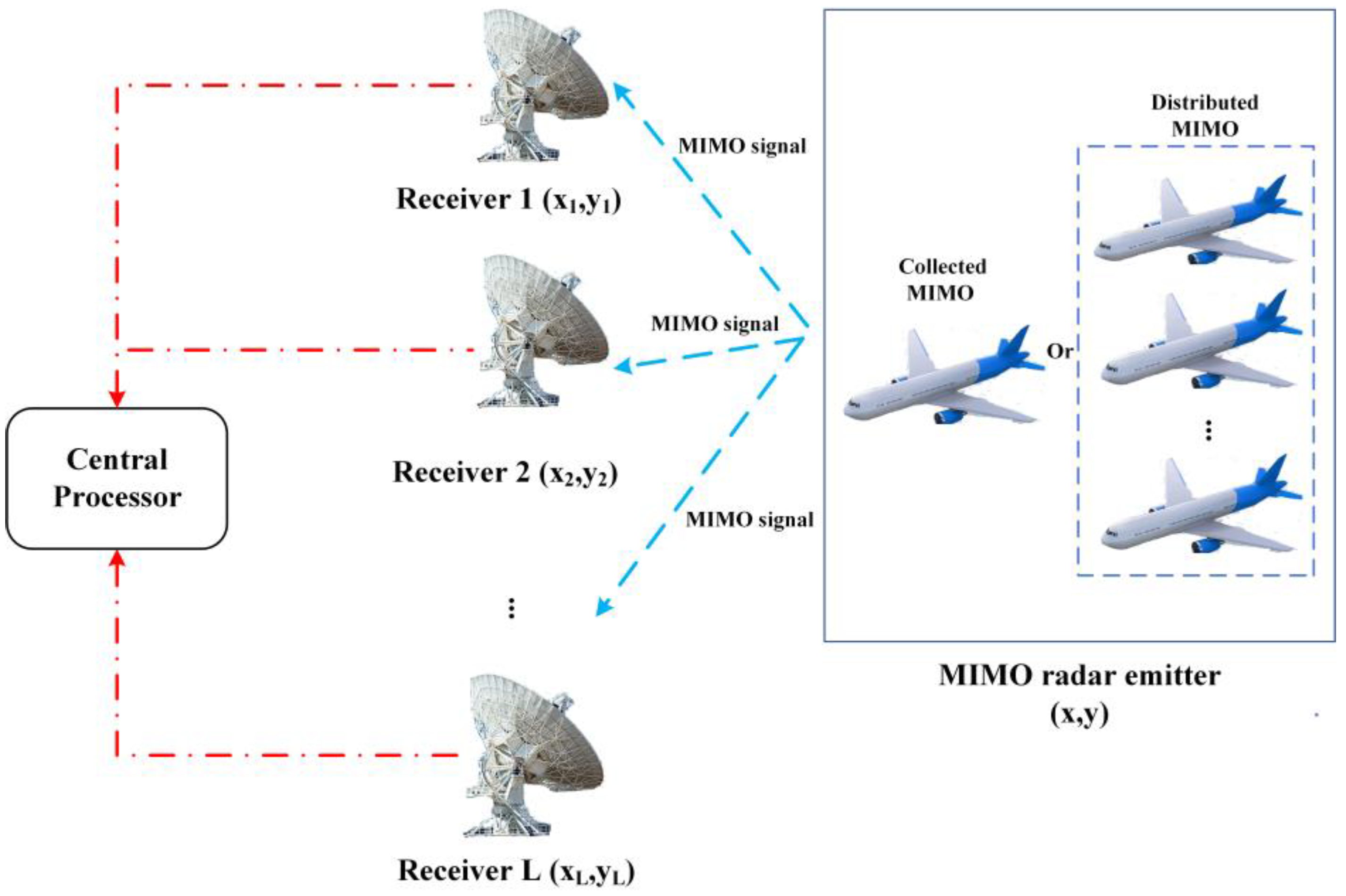
• The proposed algorithm proposes a localization framework for the distributed multi-station passive localization system, which can locate multiple signal forms.

The rest of this paper is organized as follows. Section 2 states the signal model of the MIMO radar signal emitter. In Section 3, the definitions of the DPD method are clarified and the localization problem for the MIMO radar emitter is presented. Section 4 introduces the proposed algorithm in detail. The effectiveness of the proposed algorithm was verified through simulation experiments in Section 5. Finally, the conclusion is presented in Section 6.

The conventional notations used in the paper are listed in

Table 1. The notations used in the paper.

L	the number of receiver stations
K	the number of pulses of the transmitted signal
${\mathit{r}}_{\mathit{l}}$	the observed signal for the l-th receiver station
T	the observation time
$T_s$	the pulse repetition interval
$T_q$	the pulse width
${\tau }_l\left(\mathit{p}\right)$	the delay from the emitter to the l-th receiver
${\phi }_k$	the initial phase of the k-th pulse signal
$b_l$	the attenuation coefficient of the channel
$\mathit{R}\left(\theta \right)$	the signal sample matrix
${\mathit{V}}_k\left(\theta \right)$	the noise term of the intercepted signal sample
${\rho }_k\left(\mathit{\theta }\right)$	the parameter information except the parameters to be estimated
$\mathit{U}\left(\theta \right)$	the implicit mathematical model
$\mathit{P}\left(\theta \right)$	the average power coefficient
$T_k$	the sampling time interval
$n_{l,k}^s\left(\theta \right)$	the starting index of the kth single pulse signal of the pulse sequence
$n_{l,k}^e\left(\theta \right)$	the terminal index of the kth single pulse signal of the pulse sequence
$N_{l,k}\left(\theta \right)$	the pulse width of the kth single pulse signal extracted from ${\mathit{r}}_{\mathit{l}}$.

Among the notations, L, K, T, $T_s$, $T_q$, ${\tau }_l\left(\mathit{p}\right)$, ${\phi }_k$, $b_l,$ $T_k$, $n_{l,k}^s\left(\theta \right)$, $n_{l,k}^e\left(\theta \right)$, and $N_{l,k}\left(\theta \right)$ are scalars. ${\mathit{r}}_{\mathit{l}}$ and ${\rho }_k\left(\mathit{\theta }\right)$ are vectors. $\mathit{R}\left(\theta \right)$, ${\mathit{V}}_k\left(\theta \right)$, $\mathit{U}\left(\theta \right),\mathrm{a}\mathrm{n}\mathrm{d}\mathit{P}\left(\theta \right)$ are matrices.

:

2. Signal Model

Consider a 2D Cartesian coordinate system where a non-cooperative stationary MIMO radar emitter is transmitting signals. The emitter is located at $\mathit{p}$ = (x, y). The signals are intercepted by L widely distributed receiver stations, whose coordinates are ${\mathit{p}}_l=$($x_l,y_l$), (l = 1, 2, $\cdots$, L). As shown in Figure 1, after the signals are intercepted by the base stations, they are sent to the central processor to locate the emitter. For simplicity, it is assumed that the emitter model is a collocated MIMO radar emitter [23]. The emitter radiates a pulse signal $s\left(t\right)$ outward with the pulse repetition interval (PRI) $T_s$. The transmitted signal $s\left(t\right)$ comprises K pulses $u\left(t\right)$ with pulse width $T_q$, and can be expressed as

$$s\left(t\right)={\sum }_{k=1}^{+\infty }exp\left(j{\phi }_k\right)u\left[t-\left(k-1\right)T_s\right]$$

(1)

where k is the k-th single pulse signal of the transmitted pulse sequence, and ${\phi }_k$ is the initial phase of the k-th pulse signal.

For $u\left(t\right)$, the following equation needs to be satisfied:

$$u\left(t\right)=\left\{\begin{array}{c}s\left(t\right),0\le t\le T_q\\ 0,T_q\le t\le T_s\end{array}\right.$$

(2)

The observed signal for the l-th receiver station can be expressed as

$${\mathit{r}}_{\mathit{l}}(t)=\left\{\begin{array}{c}{b}_l{s}_l\left(t\right)+{\mathit{n}}_{\mathit{l}}\left(t\right),t_{ls}\le t\le t_{le}\\ {\mathit{n}}_{\mathit{l}}\left(t\right),else\end{array}\right.$$

(3)

where $b_l$ is the attenuation coefficient of the channel between the emitter and the l-th base station. It is assumed that the observation time T is long enough, and at least one single pulse in the pulse signal $s\left(t\right)$ can be received. ${\mathit{n}}_{\mathit{l}}\left(t\right)$ represents the noise of the observed signal with covariance matrix ${\mathit{R}}_{\mathit{l}}={{\sigma }_l}^2\mathbf{I}$, where I is the identity matrix. The noise and signals are spatio-temporally uncorrelated and the receiver stations are distributed widely enough to warrant mutual independence of noise vectors,

$$\overline{{\mathit{n}}_{\mathit{l}}}\perp \overline{{\mathit{n}}_{l^{\prime }}},l\ne l^{\prime }$$

(4)

In (3), $t_{ls}$ and $t_{le}$ denote the starting and terminal times of the signal received by the l-th base station in the time duration [0, T]. $t_{ls}$ and $t_{le}$ are scalars related to the position of the base station, which can be obtained by the following formula:

$$t_l^s=t_0+{\tau }_l\left(\mathit{p}\right)$$

(5)

$$t_l^e=t_0+{\tau }_l\left(\mathit{p}\right)+T_q$$

(6)

where ${\tau }_l\left(\mathit{p}\right)$ denotes the delay from the emitter to the l-th receiver, and can be expressed as

$${\tau }_l\left(\mathit{p}\right)=\frac{\sqrt{{\left(x-x_l\right)}^2+{\left(y-y_l\right)}^2}}{c}$$

(7)

with c denoting the speed of light.

After sampling, the vector form of (3) can be expressed as

$${\mathit{r}}_{\mathit{l}}=b_l{s}_l+{\mathit{n}}_{\mathit{l}}$$

(8)

where $s_l\triangleq {\left[s_l\left[0\right]s_l\left[1\right]\cdots s_l\left[N_s-1\right]\right]}^T$,

$$\begin{gathered} {\mathit{r}}_{\mathit{l}}\triangleq {\left[{\mathit{r}}_{\mathit{l}}\left[0\right]{\mathit{r}}_{\mathit{l}}\left[1\right]\cdots {\mathit{r}}_{\mathit{l}}\left[N_s-1\right]\right]}^T, \\ {\mathit{n}}_{\mathit{l}}\triangleq {\left[{\mathit{n}}_{\mathit{l}}\left[0\right]{\mathit{n}}_{\mathit{l}}\left[1\right]\cdots {\mathit{n}}_{\mathit{l}}\left[N_s-1\right]\right]}^T \end{gathered}$$

(9)

where $N_s$ is the number of samples. ${\left[.\right]}^T$ represents the transpose operator.

3. Problem Formulation

As is indicated in [24], the unknown parameters and the position can be obtained by the ML estimator, assuming that $H_0$ corresponds to the noise hypothesis and $H_1$ corresponds to the emitters’ existence hypothesis.

For simplicity, here we assume that the noise model is the white, zero-mean complex Gaussian noise. According to [4,24,25], the likelihood function of ${\mathit{r}}_{\mathit{l}}$ corresponding to $H_0$ can be expressed as

$$p\left(\overline{\mathit{r}}|H_0\right)=C_{0}exp\left\{-\frac{1}{2}{{\mathit{r}}_{\mathit{l}}^{\mathit{H}}\mathit{R}}_{\mathit{l}}^{-1}{\mathit{r}}_{\mathit{l}}\right\}$$

(10)

Similarly, we can construct the likelihood function corresponding to $H_1$ as

$$p\left(\overline{\mathit{r}}|H_1;\mathit{p},t_0\right)={\prod }_{l=1}^{L}p\left(\overline{{\mathit{r}}_{\mathit{l}}}|H_1;\mathit{p},t_0\right)=C_1{\prod }_{l=1}^{L}exp\left\{\frac{-1}{2}{\left(\overline{{\mathit{r}}_{\mathit{l}}}-b_l\overline{s_l}\right)}^H{\mathit{R}}_{\mathit{l}}^{-1}(\overline{{\mathit{r}}_{\mathit{l}}}-b_l\overline{s_l})\right\}$$

(11)

where $C_0$ and $C_1$ are constants, and ${\left[.\right]}^H$ represents the operation of conjugation transpose.

Therefore, the likelihood ratio function can be given by

$$L\left(\overline{\mathit{r}};\mathit{p},t_0\right)=\frac{p\left(\overline{\mathit{r}}|H_1;\mathit{p},t_0\right)}{p\left(\overline{r}|H_0\right)}=\frac{C_1}{C_0}exp\left\{\frac{-1}{2}{\left(\overline{{\mathit{r}}_{\mathit{l}}}-b_l\overline{s_l}\right)}^H{\mathit{R}}_{\mathit{l}}^{-1}\left(\overline{{\mathit{r}}_{\mathit{l}}}-b_l\overline{s_l}\right)+\frac{1}{2}{\overline{{\mathit{r}}_{\mathit{l}}}}^H{\mathit{R}}_{\mathit{l}}^{-1}\overline{{\mathit{r}}_{\mathit{l}}}\right\}$$

(12)

The MLE function is based on maximizing the likelihood (12) over all attenuation coefficients $b_l$. Thus, it leads to the following ML estimation for each $b_l$ term: $b_l=\frac{{\overline{{\mathit{s}}_{\mathit{l}}}}^H{\mathit{R}}_{\mathit{l}}^{-1}\overline{{\mathit{r}}_{\mathit{l}}}}{{\overline{{\mathit{s}}_{\mathit{l}}}}^H{\mathit{R}}_{\mathit{l}}^{-1}\overline{{\mathit{s}}_{\mathit{l}}}}$.

Let $\frac{\partial L\left(r_l\right)}{\partial b_l}=0$, ${\mathit{R}}_{\mathit{l}}={{\sigma }_l}^2\mathbf{I}$, and assume ${\left|\overline{\mathrm{s}}\right|}^2=1$. After simplification, under the assumption that the signal waveform is known to the receivers, we can obtain the maximum likelihood function as follows:

$$L\left(\overline{\mathit{r}};\mathit{p},t_0\right)\propto {\sum }_{l=1}^L\left(\frac{1}{{\mathit{\sigma }}_{\mathit{l}}^2}{\left|{\overline{{\mathit{s}}_{\mathit{l}}}}^{\mathit{H}}\overline{{\mathit{r}}_{\mathit{l}}}\right|}^2\right)={\sum }_{l=1}^L\frac{1}{{\mathit{\sigma }}_{\mathit{l}}^2}{\left|{\sum }_{k=0}^{N_s-1}{e}^{j{\omega }_k\left[{\tau }_l\left(\mathit{p}\right)\right]}{\overline{s}}^{\mathrm{*}}\left[k\right]{\overline{\mathit{r}}}_l\left[k\right]\right|}^2$$

(13)

Therefore, the position of the emitter $\mathit{p}$ and the parameters of signal can be jointly estimated via the following function:

$$\widehat{\mathit{p}}=\mathit{a}\mathit{r}\mathit{g}\underset{\mathit{p}}{max}\left\{\mathrm{L}\left(\overline{\mathit{r}};\mathit{p},t_0\right)\right\}$$

(14)

From (14), it can be inferred that by conducting a grid search on the corresponding area, the position of the emitter can be estimated. For the convenience of description, the above DPD algorithm with known waveform information is referred to as the DPD-known algorithm in the following text.

If the signal waveform is not known to the receiver stations, the maximum likelihood function in (13) is not applicable. Define the following vectors:

$$\overline{{\mathit{d}}_{\mathit{l}}}\triangleq {\left[\overline{d_l}\left(0\right),\cdots ,\overline{d_l}\left(N_s-1\right)\right]}^T$$

(15)

$$\overline{\mathit{s}}\triangleq {\left[\overline{s}\left(0\right)e^{-j{\omega }_0{t}_0},\cdots ,\overline{s}\left(N_s-1\right)e^{-j{\omega }_{N_s-1}{t}_0}\right]}^T$$

(16)

where $\overline{d_l}\left(k\right)\triangleq {\mathrm{e}}^{-\mathrm{j}{\omega }_{\mathrm{k}}{\tau }_l\left(\mathit{p}\right)}{\mathit{\alpha }}_{\mathit{l}}\left(\mathit{p}\right){\overline{\mathit{r}}}_l\left(k\right)$.

Using these definitions, (12) can be equivalent to

$$\begin{gathered} \mathrm{L}\left(\overline{\mathit{r}};\mathit{p},t_0\right)=\sum _{l=1}^L{\left|{\overline{\mathit{s}}}^{\mathit{H}}{\mathit{d}}_{\mathit{l}}\right|}^2 \\ =\sum _{l=1}^L{\overline{\mathit{s}}}^{\mathit{H}}{\mathit{d}}_{\mathit{l}}{{\mathit{d}}_{\mathit{l}}}^H\overline{\mathit{s}} \\ ={\overline{\mathit{s}}}^{\mathit{H}}\left(\sum _{l=1}^L{\mathit{d}}_{\mathit{l}}{{\mathit{d}}_{\mathit{l}}}^H\right)\overline{\mathit{s}} \\ ={\overline{\mathit{s}}}^{\mathit{H}}\mathit{D}\overline{\mathit{s}} \end{gathered}$$

(17)

Here, the maximum likelihood function in (17) is maximized by selecting the vector as the eigenvector corresponding to the largest eigenvalue of the matrix $\mathit{D}$. Hence, the position of the emitter can be jointly estimated via the following function:

$$\widehat{\mathit{p}}=\mathit{a}\mathit{r}\mathit{g}\underset{\mathit{p}}{\mathit{max}}{\lambda }_{max}\left(\mathit{D}\right)$$

(18)

where ${\lambda }_{max}\left(\mathit{D}\right)$ denotes taking the largest eigenvalue of the matrix $\mathit{D}$. The matrix $\mathit{D}$ is a cost function that includes the array response at each receiver, the location of the base station, and the location of the unknown emitter.

Similar to the situation where signal waveform information is known, the maximum eigenvalue of the matrix $\mathit{D}$ can be obtained by searching the two-dimensional grid search of the corresponding region; then, the position of the emitter can be obtained. Correspondingly to the DPD-known algorithm, we refer to the DPD algorithm mentioned above in the case of an unknown signal waveform as the DPD-unknown algorithm.

It should be noted that the problem formulations of the other channel models such as Rayleigh, Rice, and non-Gaussian noise, etc., are also appropriate. As is indicated in [11,12], the localization methods are the same as (14) and (18).

Remarkably, for the MIMO radar emitter signal model, the DPD-unknown algorithm can still be used to achieve passive localization. However, because the signals transmitted by the MIMO radar emitter are multiple and independent of each other, its localization performance will obviously suffer significant losses without clear waveform information of the MIMO radar signal, especially in low signal-to-noise ratios. Therefore, in order to improve the localization accuracy of the MIMO radar emitter, it is necessary to adopt some waveform estimation methods to obtain some prior information regarding MIMO radar signals.

4. Algorithm Description

In this section, the efficient DPD approach based on KL transform and the FM technique is presented to solve the passive localization problem for MIMO radar emitters, called DPD-KL-FM for brevity. First, KL transform is employed to estimate the signal characteristics from a large number of signals observed by the receiver stations. Aiming to solve the problem that the unknown waveform of the MIMO radar emitter plagues the application of the estimator in (18) for localizing the emitter position, we propose a strategy based on the FM technique to find the target emitter and improve the performance of the parameter estimation. At last, the objective function equation of the DPD algorithm is further derived by applying a structure of the maximum Rayleigh quotient and the position of the emitter is obtained. The DPD-KL-FM algorithm is described in detail below.

4.1. Definition of KL Transform

KL transform is a feature extraction method based on statistical characteristics [26]. It has been applied and developed in the fields of feature extraction, data compression, signal noise reduction, image rotation, etc. The outstanding advantage of KL transform is the good correlation. In short, it is a simplified analysis method for the complex relationship between variables. It is a special form of orthogonal linear transformation and the best form of transformation in the sense of mean square error [27,28].

KL transform technology uses orthogonal transformation to reduce the dimension of high-dimensional data sets, that is, the random process is described as a linear combination of countless orthogonal functions, and then through the mathematical mapping relationship, the correlations between the functions or variables are converted into fewer variables. The following is a brief introduction to its mathematical principles.

Assuming that Y is the data sample to be estimated, it can be linearly represented by the observed data sample X. The column vector length of X is N, that is, X can be written as $\left\{x_1,x_2,\cdots x_N\right\}$. Then, the KL transform is defined as

$$Y=AX$$

(19)

where A is the weight coefficient matrix, which can be expressed as a vector form.

$$A\triangleq {\left[a_1,a_2,\cdots ,a_N\right]}^T$$

(20)

The weight coefficient matrix A must meet the following requirements: (1) A is an orthogonal matrix. (2) $A^{T}A=1$.

In order to make the information in the observation sample X with a length of N appear to be estimated to the greatest extent in the signal sample, according to information theory, the variance in the signal can be used to measure the amount of information, and the amount of information increases with the increase in the variance. Therefore, the weight that maximizes the variance in Y can be obtained, that is,

$$A^{\mathrm{*}}=\mathit{arg}\underset{A}{\mathit{max}}Var\left(Y\right)$$

(21)

where $Var\left(Y\right)$ can be calculated as follows:

$$Var\left(Y\right)=\frac{1}{N-1}{\sum }_{i=1}^N{\left(Y_i-\overline{x}\right)}^2$$

(22)

where $\overline{x}$ is the average value of X, which can be calculated by the following formula:

$$\overline{x}=\frac{1}{N}{\sum }_{i=1}^N{Y}_i=a_1{\overline{x}}_1+a_2{\overline{x}}_2+\cdots a_N{\overline{x}}_N$$

(23)

where ${\overline{x}}_N$ is the average of the Nth column vector of X, and ${\overline{x}}_N=\frac{1}{N}{\sum }_{i=1}^N{\overline{x}}_{N,i}$.

Substituting (23) into (22), then $Var\left(Y\right)$ can be written as

$$Var\left(Y\right)=\frac{1}{N-1}{\sum }_{i=1}^N{\left[\left(a_1{\overline{x}}_{1,i}+a_2{\overline{x}}_{2,i}+\cdots +a_N{\overline{x}}_{N,i}\right)-\left(a_1{\overline{x}}_1+a_2{\overline{x}}_2+\cdots +a_N{\overline{x}}_N\right)\right]}^2$$

(24)

After the expansion of (23), it can be simplified into the following form:

$$Var\left(Y\right)=A^T\frac{1}{N-1}{\sum }_{i=1}^N\left[\begin{array}{ccc}\begin{array}{cc}{\left(x_{1,i}-{\overline{x}}_1\right)}^2& \left(x_{1,i}-{\overline{x}}_1\right)\left(x_{2,i}-{\overline{x}}_2\right)\\ \left(x_{2,i}-{\overline{x}}_2\right)\left(x_{1,i}-{\overline{x}}_1\right)& {\left(x_{2,i}-{\overline{x}}_2\right)}^2\end{array}& \cdots & \begin{array}{c}\left(x_{1,i}-{\overline{x}}_1\right)\left(x_{N,i}-{\overline{x}}_N\right)\\ \left(x_{2,i}-{\overline{x}}_2\right)\left(x_{N,i}-{\overline{x}}_N\right)\end{array}\\ ⋮& \ddots & ⋮\\ \begin{array}{cc}\left(x_{N,i}-{\overline{x}}_N\right)\left(x_{1,i}-{\overline{x}}_1\right)& \left(x_{N,i}-{\overline{x}}_N\right)\left(x_{2,i}-{\overline{x}}_2\right)\end{array}& \cdots & {\left(x_{N,i}-{\overline{x}}_N\right)}^2\end{array}\right]A$$

(25)

Assuming that $\Sigma$ is the covariance matrix of X, its value can be expressed by the following formula:

$$\Sigma =\frac{1}{N-1}{\sum }_{i=1}^N\left[\begin{array}{ccc}\begin{array}{cc}{\left(x_{1,i}-{\overline{x}}_1\right)}^2& \left(x_{1,i}-{\overline{x}}_1\right)\left(x_{2,i}-{\overline{x}}_2\right)\\ \left(x_{2,i}-{\overline{x}}_2\right)\left(x_{1,i}-{\overline{x}}_1\right)& {\left(x_{2,i}-{\overline{x}}_2\right)}^2\end{array}& \cdots & \begin{array}{c}\left(x_{1,i}-{\overline{x}}_1\right)\left(x_{N,i}-{\overline{x}}_N\right)\\ \left(x_{2,i}-{\overline{x}}_2\right)\left(x_{N,i}-{\overline{x}}_N\right)\end{array}\\ ⋮& \ddots & ⋮\\ \begin{array}{cc}\left(x_{N,i}-{\overline{x}}_N\right)\left(x_{1,i}-{\overline{x}}_1\right)& \left(x_{N,i}-{\overline{x}}_N\right)\left(x_{2,i}-{\overline{x}}_2\right)\end{array}& \cdots & {\left(x_{N,i}-{\overline{x}}_N\right)}^2\end{array}\right]$$

(26)

Thus, (25) can be equivalent to

$$Var\left(Y\right)=A^T\Sigma A$$

(27)

It can be seen from (27) that in order to obtain the weight coefficient matrix A with $Var\left(Y\right)$ reaching its maximum value, the maximum eigenvalue of $\Sigma$ is required. The corresponding eigenvector of the eigenvalue is $A^{\mathrm{*}}$, which is required in (21).

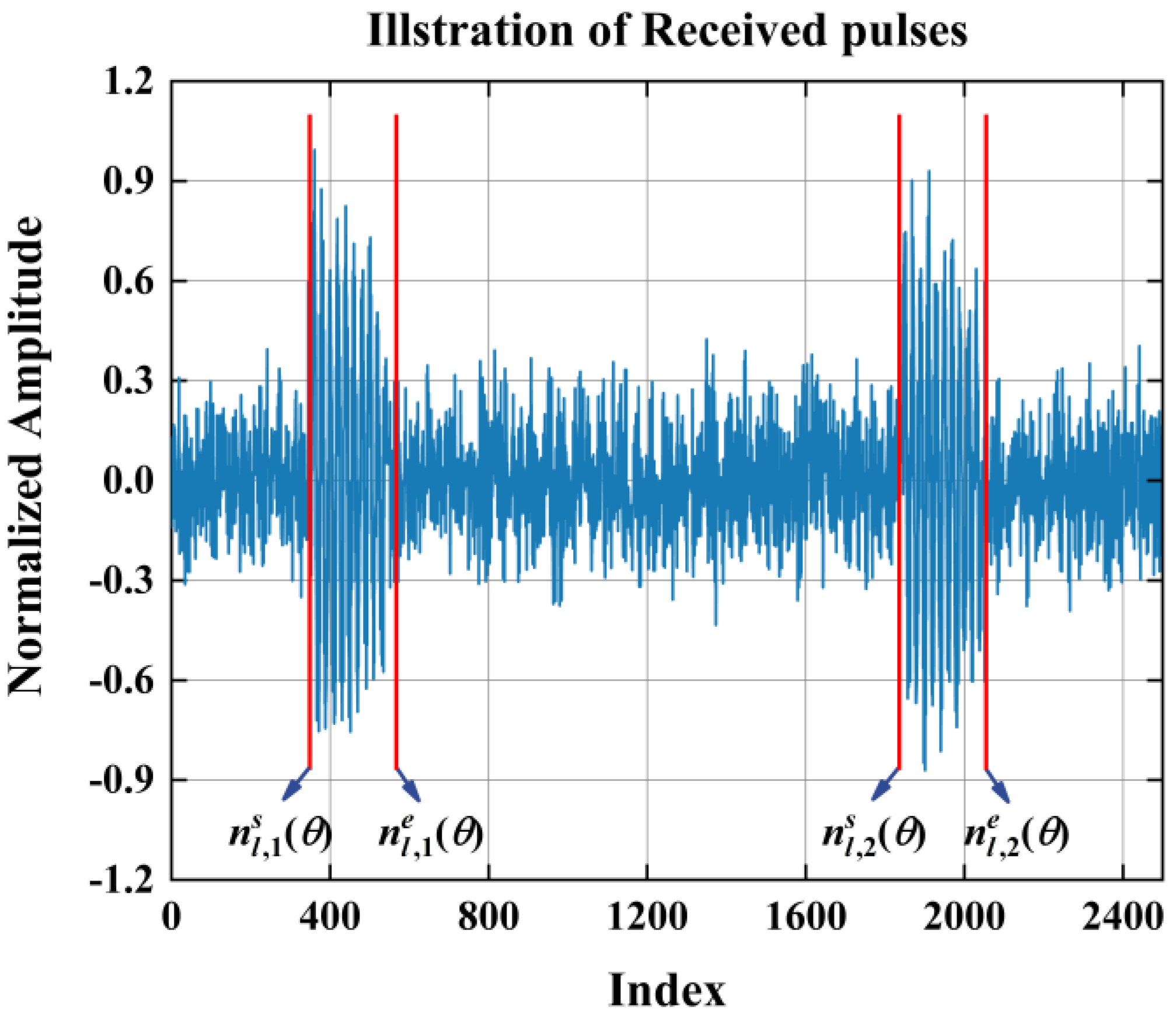
4.2. Parameter Estimation Based on KL Transform and FM

According to the principle of KL transform introduced in the previous section, after each receiving base station receives the transmitted signal of the MIMO radar signal emitter, the KL transform can be used to reduce the dimension and estimate the sample data.

Combined with the signal model of the MIMO radar emitter, the parameters of the signal ${\mathit{r}}_{\mathit{l}}\left(t\right)$ observed by the l-th receiver station include $t_0$, $T_s$, $T_q$, signal amplitude, initial phase, etc. Because the channel environment of each base station is different, the estimation of the signal amplitude is meaningless here. In order to ensure the accuracy of the localization process, the observation time is generally long, and the pulse repetition period $T_s$ is relatively small. Therefore, the number of pulses observed during the observation time is relatively large, making it difficult to estimate the phase ${\phi }_k$; so, it is no longer estimated in the KL transform. Therefore, the parameters estimated using KL transform are $t_0$, $T_s$, and $T_q$.

Firstly, the number of discrete samples of the single pulse contained in a certain observation time T (suppose that T is long enough) is estimated. Assuming that $\theta$ is the parameter to be estimated, let

$$n_l^s\left(\theta \right)=⌊\frac{T-{\tau }_l\left(\mathit{p}\right)-t_0}{T_s}⌋$$

(28)

$$n_l^e\left(\theta \right)=\frac{T-{\tau }_l\left(\mathit{p}\right)-t_0}{T_s}-n_l^s\left(\zeta \right)$$

(29)

where $⌊·⌋$ represents the operation of rounding toward minus infinity, $n_l^s\left(\theta \right)$ denotes the complete number of pulse samples, and $n_l^e\left(\theta \right)$ denotes the proportion of the pulse width of the incomplete pulse sample to the complete pulse repetition period $T_s$ in the observation time.

If it is a single pulse signal, then only $n_l^s\left(\theta \right)$ can be used to determine whether the pulse is complete. Then, $T_s$ in (28) is the observation time T. If it is a multi-pulse signal, the integrity of the pulse sample can be determined by combining the values of $n_l^s\left(\theta \right)$ and $n_l^e\left(\theta \right)$. Thus, the number of pulse samples that can be extracted by the l-th receiver station in the observation time T can be obtained as follows:

$$N_l\left(\theta \right)=\left\{\begin{array}{c}{n}_l^s\left(\theta \right),n_l^e\left(\theta \right)<D\\ n_l^s\left(\theta \right)+1,n_l^e\left(\theta \right)\ge D\end{array}\right.$$

(30)

where D is the duty cycle of the pulse signal, $D\triangleq \frac{T_q}{T_s}$.

For the kth single pulse signal of the pulse sequence, the starting index and terminal index can be calculated as follows:

$$n_{l,k}^s\left(\theta \right)=⌈\frac{t_{l,k}^s\left(\theta \right)}{T_k}⌉$$

(31)

$$n_{l,k}^e\left(\theta \right)=⌊\frac{t_{l,k}^e\left(\theta \right)}{T_k}⌋$$

(32)

where $T_k$ is the sampling time interval and $⌈·⌉$represents the operation of rounding toward infinity.

Furthermore, the pulse width of the kth single pulse signal extracted from the signal ${\mathit{r}}_{\mathit{l}}$ received by the l-th receiver station within the observation time T can be calculated by the following formula:

$$N_{l,k}\left(\theta \right)\triangleq ⌊\frac{t_{l,k}^e\left(\theta \right)-t_{l,k}^s\left(\theta \right)}{T_k}⌋=⌊\frac{T_q}{T_k}⌋$$

(33)

where $N_{l,k}\left(\theta \right)$ represents the pulse width of the kth single pulse signal extracted from ${\mathit{r}}_{\mathit{l}}$.

The $N_{l,k}\left(\theta \right)$ in (33) can also be calculated directly by $N_{l,k}\left(\theta \right)=n_{l,k}^e\left(\theta \right)-n_{l,k}^s\left(\theta \right)$, according to the definition. It can be seen from (33) that the pulse width of the single pulse signal in the signal ${\mathit{r}}_{\mathit{l}}$ is only determined by $T_q$. Therefore, $N_{l,k}\left(\theta \right)$ can also be equivalent to $N_{l,k}\left(T_q\right)$. According to (31) and (32), the discrete form of the kth monopulse signal extracted from ${\mathit{r}}_{\mathit{l}}$ can be expressed as follows:

$${\mathit{r}}_{l,k}^s\left(\theta \right)={\mathit{r}}_{\mathit{l}}\left[n_{l,k}^s\left(\theta \right):n_{l,k}^e\left(\theta \right)\right],k=\mathrm{1,2},\cdots ,N_l\left(\theta \right)$$

(34)

Considering all L receiver stations, the total number of samples finally obtained in the central processor can be represented by

$$N\left(\theta \right)={\sum }_{l=1}^L{N}_l\left(\theta \right)$$

(35)

Hence, the $N\left(\theta \right)$ pulse samples obtained by the central processor can be expressed by the following signal matrix:

$$\begin{gathered} \mathit{R}\left(\theta \right)\triangleq \left[{\mathit{r}}_{l,1}^s\left(\theta \right),{\mathit{r}}_{l,2}^s\left(\theta \right),\cdots ,{\mathit{r}}_{l,k}^s\left(\theta \right),\cdots ,{\mathit{r}}_{L,N_L\left(\theta \right)}^s\left(\theta \right)\right] \\ \triangleq \left[{\mathit{r}}_l^s\left(\theta \right),\cdots ,{\mathit{r}}_{N\left(\theta \right)}^s\left(\theta \right)\right] \end{gathered}$$

(36)

Then, applying the KL transform technique introduced in Section 4.1, the estimation of the signal can be given by

$$Y=KL\left[\mathit{R}\left(\theta \right)\right]$$

(37)

Through (37), the estimation of the signal sample for the same observation time can be obtained, $KL\left[{\mathit{R}}_{\mathit{l}}\left(\theta \right)\right]$, $l=\mathrm{1,2},\cdots ,L$. For each parameter $\theta$, L signal samples are estimated; then, feature matching is performed to determine whether it is from the same MIMO radar signal emitter. According to the system characteristics and signal characteristics of the MIMO radar emitter [29,30], the criteria for FM are as follows:

• The initial time $t_0$ of the signal is different, while the signal frequency is the same (similar within the allowable error conditions and the same below);
• The estimated value of the signal pulse width $T_q$ is the same;
• The pulse repetition interval $T_s$ of the signal is the same.

After FM, the signal that satisfies the condition can be inputted into $\mathit{R}\left(\theta \right)$, and then positioned by the improved DPD algorithm.

Figure 2 shows the simulation diagram of the signal sample interception process after KL transform and feature matching of the selected parameters. As shown in Figure 2, the red vertical line represents the intercepted signal of the MIMO radar emitter. After KL transform and FM, the difference between the emitter signal and the noise signal is significant, and thus it can be easily proposed. Based on Figure 2, Figure 3 shows the signal waveform of the extracted MIMO radar emitter samples. It can be seen that the complete waveform of the target signal is also correctly extracted, which paves the way for the subsequent positioning process.

4.3. Design of the Localization Algorithm

Recall that, in Section 3, the localization accuracy DPD-unknown algorithm was poor due to the lack of prior information on the signal waveform. For MIMO radars that transmit orthogonal or non-coherent waveforms, the shortcomings of the DPD-unknown algorithm will be amplified more obviously. Therefore, in view of the above problems, a DPD algorithm based on KL transform and feature matching (DPD-KL-FM) is proposed in this section. The proposed approach can estimate and locate the MIMO radar emitter signal through the distributed multi-station passive localization system without prior information, such as the emitter and its waveform information. The DPD-KL-FM algorithm is introduced in detail below.

For the signal sample matrix $\mathit{R}\left(\theta \right)$ estimated using KL transform and FM in Section 4.2, one section is intercepted and can be written as follows:

$${\mathit{R}}_k\left(\theta \right)={\rho }_k\left(\mathit{\theta }\right)\mathit{U}\left(\theta \right)+{\mathit{V}}_k\left(\theta \right),k=\mathrm{1,2},\cdots ,N\left(\theta \right)$$

(38)

where $\mathit{U}\left(\theta \right)$ is the implicit mathematical model corresponding to $\mathit{R}\left(\theta \right)$, ${\mathit{V}}_k\left(\theta \right)$ is the noise term of the intercepted signal sample ${\mathit{R}}_k\left(\theta \right)$, and ${\rho }_k\left(\mathit{\theta }\right)$ denotes the parameter information except the parameters to be estimated, such as initial phase, complex attenuation coefficient, etc.

Note that the value of $\mathit{U}\left(\theta \right)$ varies with the parameter $\theta$. Therefore, only when the feature matching is successful is the model’s estimation of all pulse samples consistent, which also reflects the importance of the FM process in signal estimation and subsequent localization performance.

For the convenience of later expression, (37) is written as the following matrix form,

$$\mathit{R}=\mathit{U}{\rho }^T+\mathit{V}$$

(39)

where $\mathit{R}=\left[{\mathit{r}}_1^s,\cdots ,{\mathit{r}}_{N\left(\theta \right)}^s\right]$,$\rho ={\left[{\rho }_1,\cdots ,{\rho }_1\right]}^T$,$\mathrm{a}\mathrm{n}\mathrm{d}\mathit{V}=\left[{\mathit{V}}_1,\cdots ,{\mathit{V}}_{N\left(\theta \right)}\right]$.

For the sample signal model of the MIMO radar emitter in (39), the estimation of $\mathit{U}$ is transformed into an optimization problem by using the least square method. The objective function of the optimization problem is as follows:

$$\underset{\mathit{U},\mathit{\rho }}{\mathit{min}}{‖\mathit{R}-\mathit{U}{\mathit{\rho }}^{\mathit{T}}‖}_{\mathit{F}}^2$$

(40)

where ${‖·‖}_F$ denotes the Frobenius norm.

According to the definition of the Frobenius norm, (40) can be equivalent to

$$\underset{\mathit{U},\rho }{\mathit{min}}tr\left[{\left(\mathit{R}-\mathit{U}{\rho }^T\right)}^H\left(\mathit{R}-\mathit{U}{\rho }^T\right)\right]$$

(41)

Then, the following objective function can be constructed to solve the problem,

$$\mathit{f}\left(\mathit{U},\mathit{\rho }\right)=\mathit{t}\mathit{r}\left[{\mathit{R}}^{\mathit{H}}\mathit{R}-{\mathit{R}}^{\mathit{H}}\mathit{U}{\mathit{\rho }}^{\mathit{T}}-{\mathit{\rho }}^{\mathit{*}}{\mathit{U}}^{\mathit{H}}\mathit{R}+{\mathit{\rho }}^{\mathit{*}}{\mathit{U}}^{\mathit{H}}\mathit{U}{\mathit{\rho }}^{\mathit{T}}\right]$$

(42)

According to the matrix theory, the minimum value of $f\left(\mathit{U},\rho \right)$ can be obtained when point $\rho$ is equal to zero,

$${\nabla }_{\mathit{\rho }}\mathit{f}\left(\mathit{U},\mathit{\rho }\right){|}_{\mathit{\rho }=\widehat{\mathit{\rho }}}=0$$

(43)

The implicit model of the signal sample matrix $\mathit{R}\left(\theta \right)$ can be obtained by (43); then, the estimated value of $\mathit{U}$, which contains the signal waveform information, can be estimated as follows:

$$\widehat{\mathit{U}}=\underset{\mathit{U}}{\mathit{max}}\frac{{\mathit{U}}^{\mathit{H}}\mathit{R}{\mathit{R}}^{\mathit{H}}\mathit{U}}{{‖\mathit{U}‖}_2^2}$$

(44)

According to the Cayley–Hamilton theorem in matrix theory and the solution of the maximum value of the Rayleigh quotient in the Hermite matrix, $\widehat{\mathit{U}}$ can be obtained as follows:

$$\widehat{\mathit{U}}={\mathit{\vartheta }}_{{\mathit{\lambda }}_{\mathit{m}\mathit{a}\mathit{x}}\left(\mathit{R}{\mathit{R}}^{\mathit{H}}\right)}$$

(45)

where ${\lambda }_{max}\left(\mathit{R}{\mathit{R}}^H\right)$ denotes the maximum value of matrix $\mathit{R}{\mathit{R}}^H$, and ${\vartheta }_{{\lambda }_{max}\left(\mathit{R}{\mathit{R}}^H\right)}$ is the corresponding eigenvector of the eigenvalue.

After estimating the signal waveform of the MIMO radar emitter, the DPD algorithm can be used for localization. Since the scenario assumed in this paper is that the waveform information of the MIMO radar emitter is unknown, we can improve the model of the DPD-unknown algorithm in Section 3 for the localization of the MIMO radar emitter.

According to the previous derivation, for MIMO radar emitters, the objective function $\mathit{D}\left(\theta \right)$ can be written as

$$\mathit{D}\left(\mathit{\theta }\right)={\sum }_{\mathit{l}=1}^{\mathit{L}}{\sum }_{\mathit{k}=1}^{{\mathit{N}}_{\mathit{l}}}{\left|{\mathit{r}}_{\mathit{l},\mathit{k}}^{\mathit{H}}\left(\mathit{\theta }\right){\widehat{\mathit{U}}}_{\mathit{l},\mathit{k}}\left(\mathit{\theta }\right)\right|}^2$$

(46)

where ${\mathit{r}}_{l,k}^{\mathrm{H}}\left(\theta \right)$ represents the signal fragment of the non-zero part of the k-th pulse sample ${\widehat{\mathit{U}}}_{l,k}\left(\theta \right)$ in the signal ${\mathit{r}}_{\mathit{l}}$ received by the l-th receiver station.

Obviously, for (46), the value of $\mathit{D}\left(\theta \right)$ increases with the growth of the search pulse width $T_q$, which will lead to a decrease in the accuracy of the parameter estimation. The reason for this is that as the number of pulse samples increases, more noise samples are also brought, which reduces the parameter estimation and localization accuracy. In order to solve the contradiction between the pulse width and the parameter estimation accuracy, the average power coefficient $\mathit{P}\left(\theta \right)$ is introduced. $\mathit{P}\left(\theta \right)$ is defined as follows:

$$\mathit{P}\left(\theta \right)=\frac{{‖{\widehat{\mathit{U}}}_{l,k}\left(\theta \right)‖}_2^2}{T_q}$$

(47)

Equation (47) represents the average energy of the MIMO radar emitter signal sample ${\widehat{\mathit{U}}}_{l,k}\left(\theta \right)$ estimated within the search pulse width $T_q$. Then, a new objective function $\mathit{D}\left(\theta \right)$ can be obtained,

$$\tilde{\mathit{D}}\left(\theta \right)=\mathit{P}\left(\theta \right)\mathit{D}\left(\theta \right)$$

(48)

In summary, the estimator for the MIMO radar emitter can be expressed as

$$\widehat{\mathit{p}}=\mathit{a}\mathit{r}\mathit{g}\underset{\mathit{p}}{max}{\lambda }_{max}\left(\tilde{\mathit{D}}\left(\theta \right)\right)$$

(49)

The general pseudo-codes of the proposed DPD-KL-FM algorithm are provided in Algorithm 1.

Algorithm 1 The DPD-KL-FM algorithm.

Input: System parameter $\mathit{D}\left(\theta \right)$; observation signal sample r

1. Obtain the signal from the base stations and sample it to obtain L discrete vectors;     2. The sample vector of each single pulse signal is extracted from all of the received signal samples and a matrix is formed;     3. The signal samples are reduced and estimated via KL transform and FM;     4. The signal samples of the same MIMO radar emitter are determined via FM;     5. Reconstruct signal sample by (45) according to the estimated parameters $n_{l,k}^s\left(\theta \right),n_{l,k}^e\left(\theta \right)$, etc.;     6. For each grid point:

Calculate the average power coefficient and objective function value;

Calculate $\tilde{\mathit{D}}\left(\theta \right)$ and replace $\mathit{D}\left(\theta \right)$ with $\tilde{\mathit{D}}\left(\theta \right)$.

End

7. Maximize $\mathit{D}\left(\theta \right)$ and compute the position of the MIMO radar emitter using (49)

Output: The position of the MIMO radar emitter $\widehat{\mathit{p}}$.

4.4. Analysis of Complexity

The complexity of the DPD-KL-FM algorithm is composed of the complexity of a two-dimensional search and complexity of maximum likelihood estimation. The overall computational complexity of the DPD algorithm is $\mathrm{O}\left(N_x{N}_y{N}_p{N}_{\tau }\left((L{N}_s\left(N_s+1\right)+O_f\left(L,N_s\right))\right)\right)$, where $N_s$, $N_x$, and $N_y$ denote the number of samples and the number of meshes on the x-axis and y-axis, respectively. Since the KL transform and FM technique are used to reduce the dimension and estimate the sample data, the overall computational complexity of the DPD-KL-FM algorithm is $\mathrm{O}\left(N_{to}{N}_{Tq}{N_{Ts}N}_x{N}_y\right)$, where $t_0$, $T_s$, and $T_q$ are the selected parameters estimated using KL transform and the FM technique. Therefore, the complexity is determined using a two-dimensional grid search and the parameters selected for KL transform and the FM technique.

5. Simulation Results and Discussion

In this section, the performance of the proposed DPD-KL-FM algorithm is analyzed and verified via simulation experiments. The analysis is mainly conducted from the following two aspects: Firstly, the influence of KL transform and the FM technique on MIMO radar signal estimation is tested. The second aspect is to use Monte Carlo experiments to verify the positioning performance of the proposed algorithm.

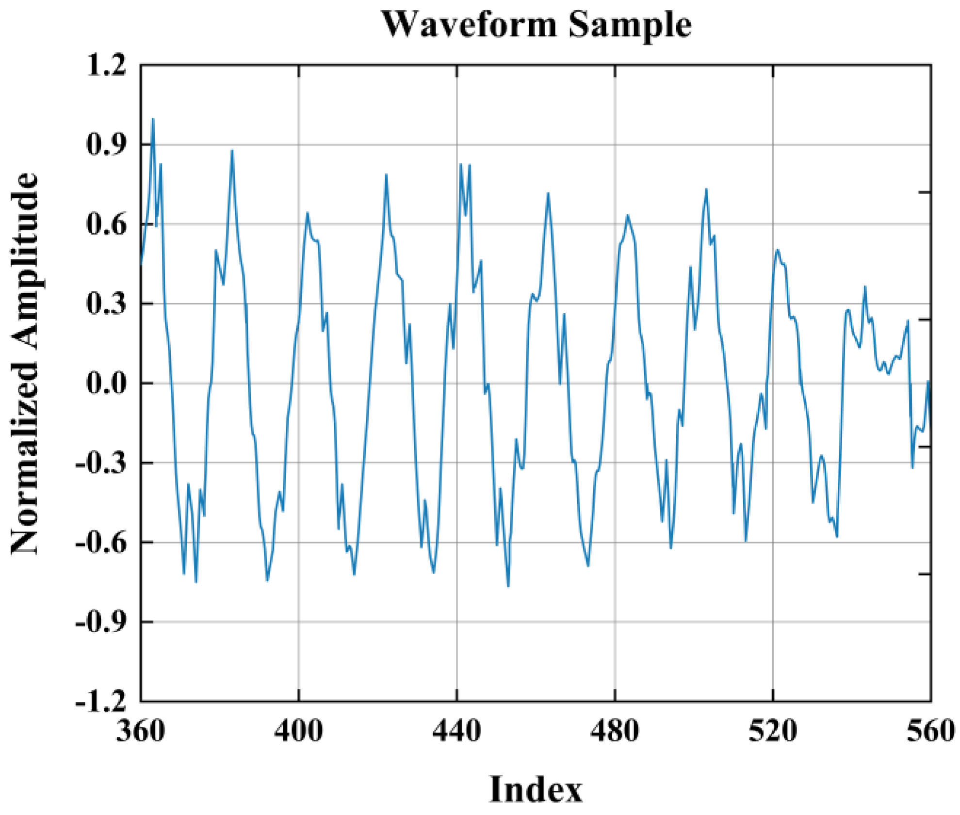
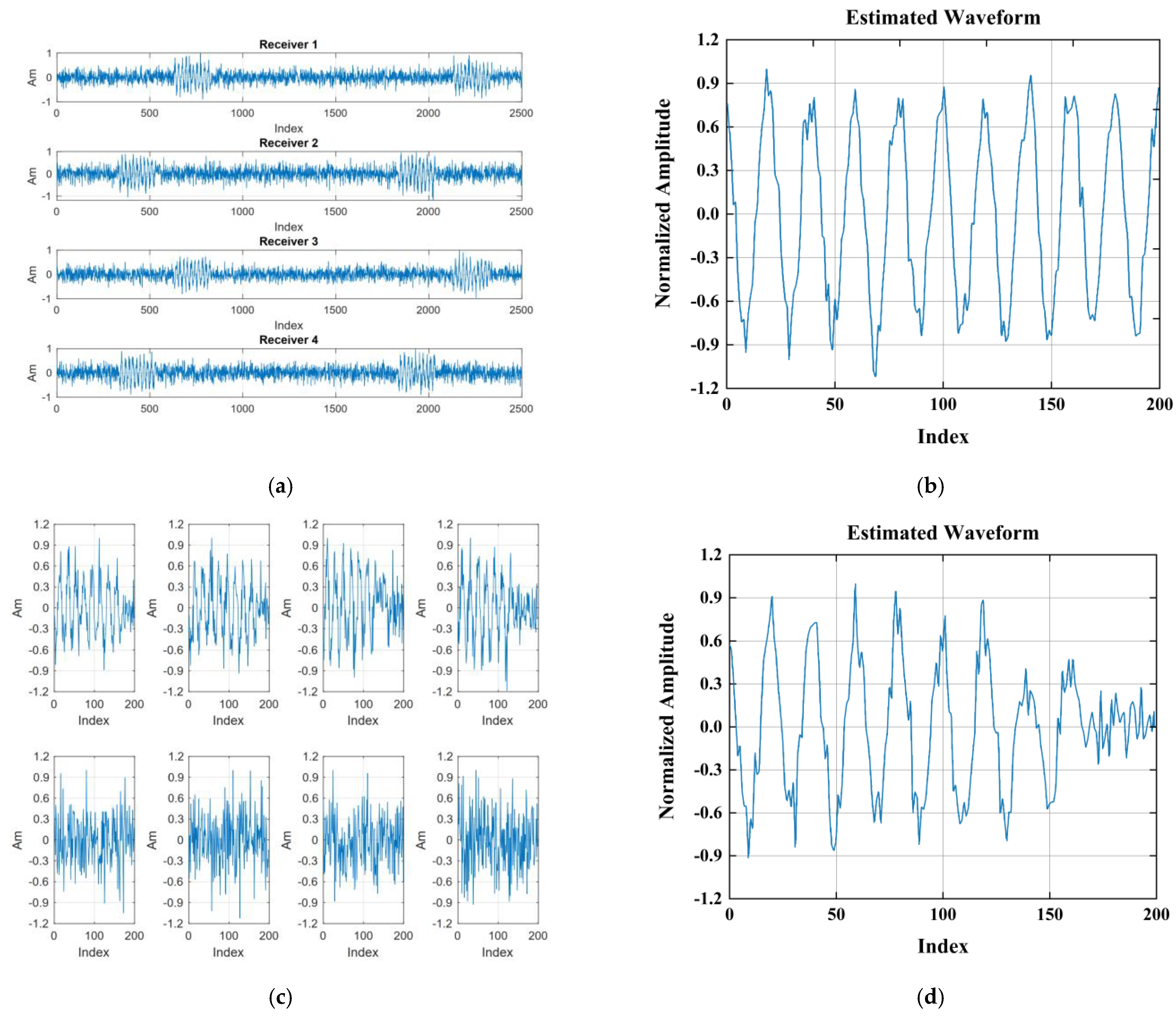
5.1. Effect of KL Transform and FM Technique on Waveform Estimation

As shown in Figure 4, the coordinates of the four base stations in the simulation are set to (0, 0) m, (12,000, 0) m, (12,000, 12,000) m, and (4800, 12,000) m, and a collocated MIMO radar emitter is located at (5000, 6000) m. In the experiment, the Gaussian pulse with pulse width $T_q=5\mathsf{\mu }\mathrm{s}$ is selected as the MIMO radar emitter signal, and the frequency of the carrier signal is $f_0=3\mathrm{M}\mathrm{H}\mathrm{z}$. Other simulation parameters are shown in

Table 2. Simulation parameters.

Signal Parameters	Parameter Value
Pulse width $T_q$	$5\mathsf{\mu }\mathrm{s}$
Pulse repetition interval $T_s$	$150\mathsf{\mu }\mathrm{s}$
Starting time $t_0$	$10\mathsf{\mu }\mathrm{s}$
Sampling frequency $f_s$	$10\mathrm{M}\mathrm{H}\mathrm{z}$
The frequency of the carrier signal $f_0$	$3\mathrm{M}\mathrm{H}\mathrm{z}$
Time duration T	1 ms

.

According to the above parameters, the single pulse signal in the signal ${\mathit{r}}_{\mathit{l}}$ received by the l-th receiver station can be expressed as

$$s_l\left(t\right)={\left(\frac{1}{T_q}\right)}^{\frac{1}{4}}exp\left(-\frac{\pi t^2}{{T_q}^2}\right)exp\left(j2\pi f_{0}t\right),0\le t\le T_q$$

(50)

Figure 2 and Figure 3 in the previous section show the simulation diagrams of the signal sample interception process after KL transform and feature matching of the selected parameters and the extracted MIMO radar emitter signal waveform. In order to reflect the effect of KL transform and feature matching on signal waveform estimation more intuitively, Figure 5 gives the simulation diagram of signal sample interception and waveform estimation without KL transform and FM.

Since the signal noise without KL transform and feature matching has a great influence on the target emitter signal, in order to more generally present the gain effect of the proposed algorithm on the emitter signal samples in the figure, two signal samples with index numbers of 0–200 were randomly intercepted for the signals received by each base station, as shown in Figure 5; by comparing Figure 5a,c, it can be seen that the proposed method can distinguish the signal of the MIMO emitter well from the noise, so as to facilitate the extraction and estimation of the target signal samples. The signal without KL transform and feature matching is more disorderly. Comparing Figure 5b,d, it can be found that the signal sample waveform of the MIMO radar emitter after KL transform and feature matching is estimated more accurately. As shown in Figure 5, the samples estimated without KL transform and feature matching are seriously damaged by noise.

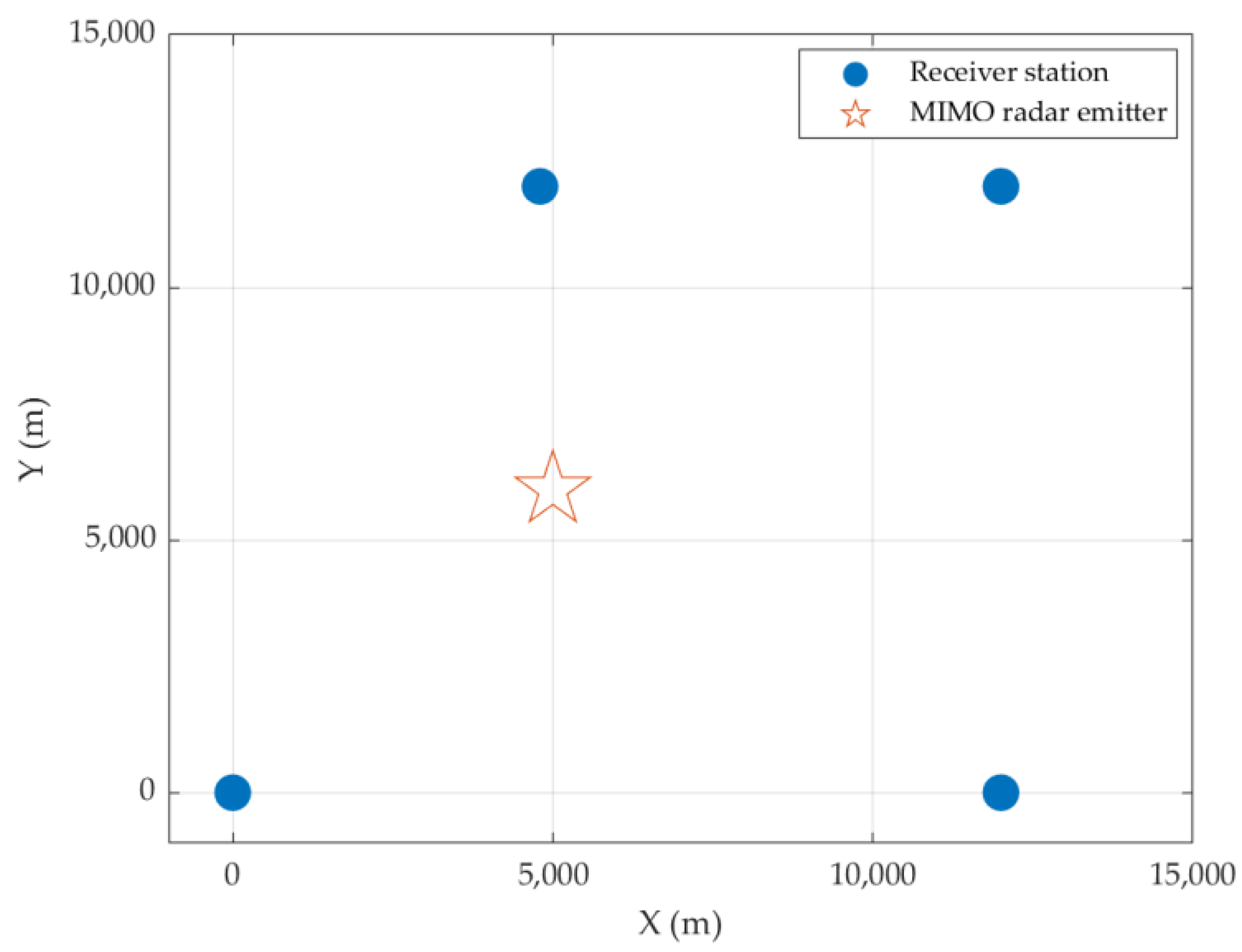
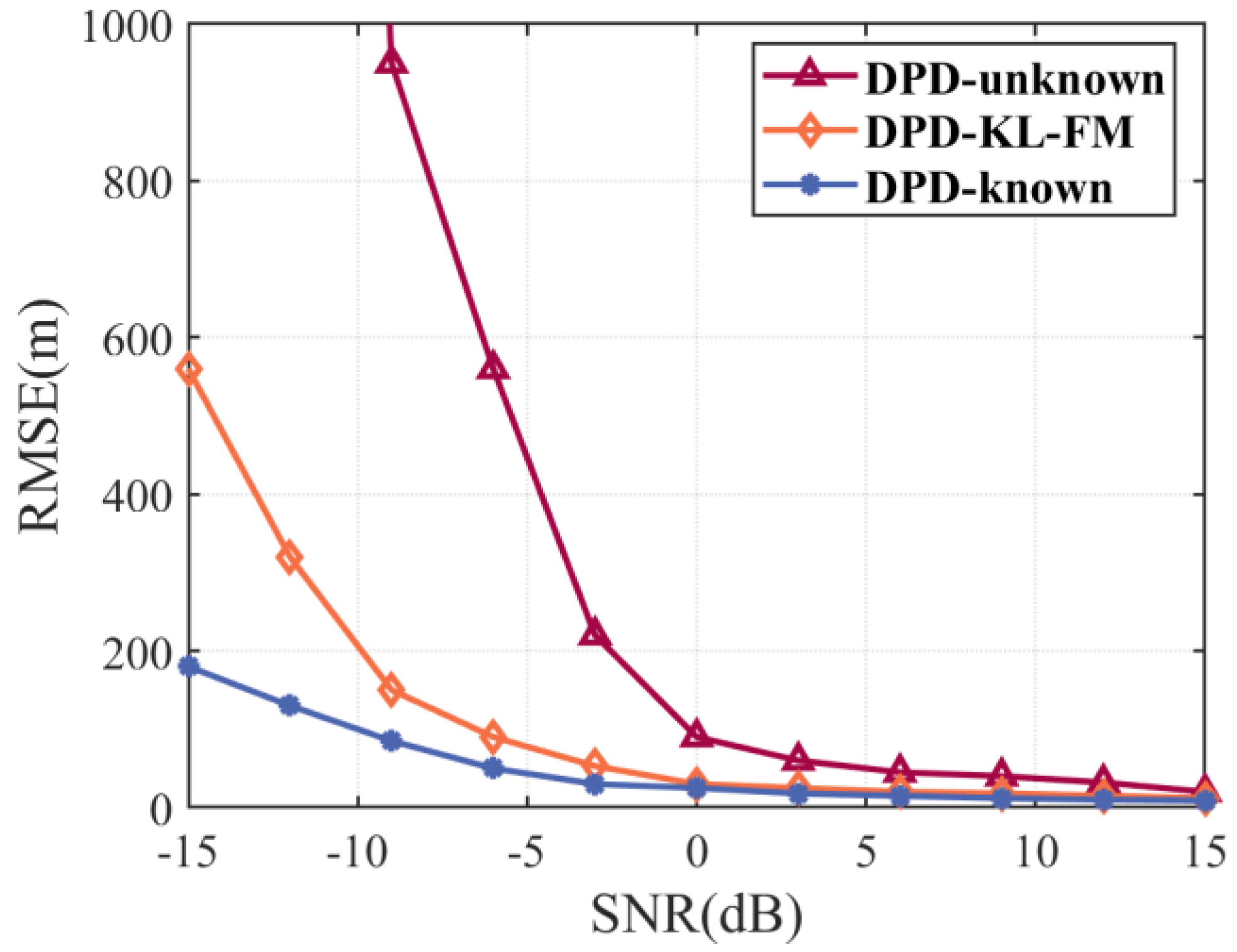
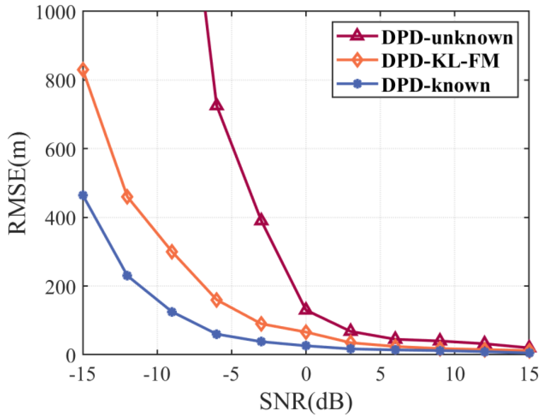
5.2. Algorithm Localization Performance Analysis

In this section, the localization performance of the proposed DPD-KL-FM algorithm is further analyzed and verified by Monte Carlo experiments. The DPD-known and DPD-unknown algorithms introduced in Section 3 are used as comparison algorithms. Since the DPD-known algorithm is based on the maximum likelihood estimation that the transmitted signal information is completely known by the base stations, the DPD-known algorithm can be considered to be completely known without estimation for the features used for KL transform and FM, such as $t_0$, $T_q$, etc. Hence, the performance of DPD-known can be viewed as an upper bound for the performance of the proposed approach and the DPD-unknown algorithm.

For each Monte Carlo experiment, we assume that the error between the estimated position $\widehat{\mathit{p}}=\left(\widehat{x_l},\widehat{y_l}\right)$ of the emitter and the actual position $\mathit{p}=\left(x,y\right)$ is calculated as follows:

$${\mathit{E}}_{\mathit{i}}=\sqrt{{(\widehat{x_i}-x)}^2+{(\widehat{y_i}-y)}^2}$$

(51)

where ${\mathit{E}}_{\mathit{i}}$ is the estimation of the emitter position of the i-th Monte Carlo trial.

The root mean square error (RMSE) of the estimated parameter is defined as

$$RMSE=\sqrt{\frac{1}{M}{\sum }_i^M{‖\widehat{\mathit{p}}-\mathit{p}‖}^2}\times 100\%$$

(52)

Two kinds of signals commonly used in MIMO radar emitters, rectangular square wave signal and Gaussian signal, were selected as representatives to verify the performance of the DPD-KL-FM algorithm. In these numerical examples below, the RMSE was computed on 500 independent experiments.

The expression of the Gaussian pulse signal is given in (49), and the relevant signal parameters remain consistent with those listed in Section 5.1, which describe the root mean square error of the three algorithms at different SNRs. As shown in Figure 6, when the SNR is high, the RMSEs of the three algorithms are low and they all maintain good localization accuracy, and the localization performance is almost the same when the SNR is greater than 0 dB. However, as the SNR decreases, the localization performance of the DPD-unknown algorithm deteriorates quickly. When the SNR is below −5 dB, even if the SNR changes slightly, the value of RMSE will fluctuate greatly. In contrast, the performance of the proposed DPD-KL-FM algorithm is relatively stable. When the SNR is above −10 dB, it is very close to the upper bound of the localization performance, which proves the gain effect of KL transform and the FM technique on the dimensionality reduction and estimation of MIMO radar emitter signal samples.

In order to further test the performance of the DPD-KL-FM algorithm, the following simulation experiments were carried out with a rectangular square wave signal as an example. The parameters such as pulse width and center frequency of the signal are the same as the above simulation experiments. The expression of rectangular square wave signal is as follows:

$$s_l\left(t\right)=exp\left(j2\pi f_{0}t\right),0\le t\le T_q$$

(53)

Figure 7 shows the change in RMSEs with the SNR when the transmitted waveform of the MIMO radar emitter is rectangular square wave. Note that the simulation experiments of Figure 6 and Figure 7 were conducted with Gaussian noise and non-Gaussian noise (impulse noise, Rice noise, etc.) and there is almost no difference in the experimental results. Here, we did not provide localization performance figures for each of the two scenarios; thus, Figure 6 and Figure 7 can be considered as the average of the two situations. Similar to the case of Gaussian signals, the proposed DPD-KL-FM algorithm maintains excellent localization performance. Compared with the DPD-unknown algorithm, the localization performance is significantly improved, especially with a low SNR. More specifically, when the SNR is −6 dB, the RMSE of the DPD-KL-FM algorithm is still less than 200 m, which is close to the upper bound of the positioning performance. At this time, the RMSE of the DPD-unknown algorithm exceeds 700 m. With a decrease in the SNR, the localization performance gap will continue to expand. Therefore, it can be concluded that the localization performance of the DPD-KL-FM algorithm is still far better than that of the DPD-unknown algorithm when the transmitted signal of the MIMO radar is rectangular square wave.

6. Conclusions

Aiming at solving the localization problem of MIMO radar emitters, especially when the waveform information transmitted by MIMO radar emitters is completely unknown, this paper proposed a novel DPD algorithm based on KL transform and FM techniques to localize MIMO radar emitters with distributed receiver stations. To achieve highly accurate and robust localization performance when the transmitted signal is unknown for receiver stations, KL transform and FM can be adopted to jointly estimate the emitter position and the unknown signal waveform. Moreover, the MIMO radar emitter can be found by matching the estimated signal parameter features, so as to effectively utilize the emitter signal information and eliminate the influence of noise on the localization performance. The simulation results verify the effectiveness of the proposed algorithm.

The main limitation of this paper is that there is a trade-off between localization performance and implementation complexity. Moreover, for more complicated scenes, such as the distribution of the receiver stations being irregular or the multi-path not being negligible, further work is underway to consider the boundary conditions and algorithms with less computational complexity.

References

1. Pan, J. Multi-station TDOA Localization Method Based on Tikhonov Regularization. In Proceedings of the 2022 7th International Conference on Intelligent Computing and Signal Processing (ICSP), Xi’an, China, 15–17 April 2022; IEEE: Piscataway, NJ, USA, 2022; pp. 1903–1906. [Google Scholar]
2. Zhang, Q.; Li, J.; Tang, Y.; Deng, W.; Zhang, X. A Direct Position Determination Method under Unknown Multi-Perturbation with Moving Distributed Arrays. Electronics 2023, 12, 1016. [Google Scholar] [CrossRef]
3. So, H.C. Source localization: Algorithms and analysis. In Handbook of Position Location: Theory, Practice, and Advances; Wiley: Hoboken, NJ, USA, 2011; pp. 25–66. [Google Scholar]
4. Zhang, S.; Jiang, H.; Yang, K. Detection and localization for an unknown emitter using TDOA measurements and sparsity of received signals in a synchronized wireless sensor network. In Proceedings of the 2013 IEEE International Conference on Acoustics, Speech and Signal Processing, Vancouver, UK, 26–31 May 2013; pp. 5146–5149. [Google Scholar]
5. Dong, H.; Yin, C.; Zhang, Y. Research on RSS Based Multi Station Passive Location Method for Satellite Emitter. In Proceedings of the 2022 IEEE 10th International Conference on Information, Communication and Networks (ICICN), Zhangye, China, 19–22 August 2022; IEEE: Piscataway, NJ, USA, 2022; pp. 147–151. [Google Scholar]
6. Bilgi Akdemir, S. An Overview of Detection in MIMO Radar. Master’s Thesis, Middle East Technical University, Ankara, Turkey, 2010. [Google Scholar]
7. Fishler, E.; Haimovich, A.; Blum, R.; Chizhik, D.; Cimini, L.; Valenzuela, R. MIMO radar: An idea whose time has come. In Proceedings of the 2004 IEEE Radar Conference (IEEE Cat. No.04CH37509), Philadelphia, PA, USA, 29 April 2004; pp. 71–78. [Google Scholar]
8. Fletcher, A.S.; Robey, F.C. Performance bounds for adaptive coherence of sparse array radar. In Proceedings of the 12th Annual Workshop on Adaptive Sensor Array Processing; Massachusetts inst of tech Lexington Lincoln lab Lexington, Lexington, MA, USA; 2003. [Google Scholar]
9. Bekkerman, I.; Tabrikian, J. Target Detection and Localization Using MIMO Radars and Sonars. IEEE Trans. Signal Process. 2006, 54, 3873–3883. [Google Scholar] [CrossRef]
10. Hack, D.E.; Patton, L.K.; Himed, B.; Saville, M.A. Detection in Passive MIMO Radar Networks. IEEE Trans. Signal Process. 2014, 62, 2999–3012. [Google Scholar] [CrossRef]
11. Weiss, A.J. Direct position determination of narrowband radio transmitters. IEEE Signal Process. Lett. 2004, 11, 513–516. [Google Scholar] [CrossRef]
12. Amar, A.; Weiss, A.J. Direct position determination (DPD) of multiple known and unknown radio-frequency signals. In Proceedings of the 2004 12th European Signal Processing Conference, Vienna, Austria, 6–10 September 2004; pp. 1115–1118. [Google Scholar]
13. Chen, F.; Zhou, T.; Yi, W.; Kong, L.; Guo, S. Passive direct positioning of emitters with unknown LFM signals based on FRFT. In Proceedings of the 2018 IEEE Radar Conference (RadarConf18), Oklahoma City, OK, USA, 23–27 April 2018; pp. 1134–1139. [Google Scholar]
14. Zhao, C.; Ke, W.; Wang, T. Multi-target localization using distributed MIMO radar based on spatial sparsity. In Proceedings of the 2021 IEEE International Conference on Artificial Intelligence and Computer Applications (ICAICA), Dalian, China, 28–30 June 2021; pp. 591–595. [Google Scholar]
15. Sadeghi, M.; Behnia, F.; Amiri, R.; Farina, A. Target Localization Geometry Gain in Distributed MIMO Radar. IEEE Trans. Signal Process. 2021, 69, 1642–1652. [Google Scholar] [CrossRef]
16. Buzzi, S.; Grossi, E.; Lops, M.; Venturino, L. Foundations of MIMO Radar Detection Aided by Reconfigurable Intelligent Surfaces. IEEE Trans. Signal Process. 2022, 70, 1749–1763. [Google Scholar] [CrossRef]
17. Kafshgari, S.; Andargoli, S.M.H. Closed-form CRLB and LPI power allocation strategies for MIMO radars with unneglectable clutter. Phys. Commun. 2023, 58, 102011. [Google Scholar] [CrossRef]
18. Xiong, K.; Cui, G.; Yi, W.; Wang, S.; Kong, L. Distributed Localization of Target for MIMO Radar with Widely Separated Directional Transmitters and Omnidirectional Receivers. IEEE Trans. Aerosp. Electron. Syst. 2022, 59, 3171–3187. [Google Scholar] [CrossRef]
19. Gogineni, S.; Nehorai, A. Target estimation using sparse modeling for distributed MIMO radar. IEEE Trans. Signal Process. 2011, 59, 5315–5325. [Google Scholar] [CrossRef]
20. Sun, B.; Chen, H.; Wei, X.; Li, X. Multitarget direct localization using block sparse bayesian learning in distributed MIMO radar. Int. J. Antennas Propag. 2015, 2015, 903902. [Google Scholar] [CrossRef] [Green Version]
21. Eshkevari, A.; Sadough, S.M.S. An Improved Method for Localization of Wireless Capsule Endoscope Using Direct Position Determination. IEEE Access 2021, 9, 154563–154577. [Google Scholar] [CrossRef]
22. Ni, L.; Wu, R.; Yang, J.; Chen, J.; Wan, Q. Fast Direct-Position-Determination based on PSO. In Proceedings of the IGARSS 2022-2022 IEEE International Geoscience and Remote Sensing Symposium, Kuala Lumpur, Malaysia, 17–22 July 2022; pp. 1971–1974. [Google Scholar]
23. Radmard, M.; Karbasi, S.M.; Nayebi, M.M. MIMO localization by illuminators of opportunity. In Proceedings of the 2011 IEEE CIE International Conference on Radar, Chengdu, China, 24–27 November 2011; Volume 1, pp. 112–115. [Google Scholar]
24. Schonhoff, T.A.; Giordano, A.A. Detection and Estimation Theory and its Applications; Pearson College Division: Drive Victoria, BC, Canada, 2006. [Google Scholar]
25. Ren, H.; Liu, H.; Guo, R. A Fast Direct Position Determination Algorithm for LFM Signal Based on Spectrum Detection. J. Sens. 2022, 2022, 2222247. [Google Scholar] [CrossRef]
26. Sanchez-Marin, F. Computerized recognition of biological objects using the Hotelling transform. In Proceedings of the 22nd Annual International Conference of the IEEE Engineering in Medicine and Biology Society (Cat. No.00CH37143), Chicago, IL, USA, 23–28 July 2000; Volume 4, pp. 3067–3070. [Google Scholar]
27. Xue, X.; Zheng, Y. A method based on wavelet transform and discrete KL transform for color image filtering. In Proceedings of the 2010 2nd International Conference on Signal Processing Systems, Dalian, China, 5–7 July 2010; IEEE: Piscataway, NJ, USA, 2010; Volume 2, pp. V2-699–V2-701. [Google Scholar]
28. Du, B.; Geng, X.; Ding, Q. Generation and realization of digital chaotic key sequence based on KL transform. In Proceedings of the 2011 Fourth International Workshop on Chaos-Fractals Theories and Applications, Hangzhou, China, 19–22 October 2011; IEEE: Piscataway, NJ, USA, 2011; pp. 385–389. [Google Scholar]
29. Li, J.; Stoica, P. MIMO Radar Signal Processing; John Wiley & Sons: Hoboken, NJ, USA, 2008. [Google Scholar]
30. Sun, H.; Brigui, F.; Lesturgie, M. Analysis and comparison of MIMO radar waveforms. In Proceedings of the 2014 International Radar Conference, Lille, France, 13–17 October 2014; IEEE: Piscataway, NJ, USA, 2014; pp. 1–6. [Google Scholar]
Figure 1. MIMO radar emitter localization scenario diagram.
Electronics 12 02971 g001
Figure 2. The signal waveform of the extracted MIMO radar emitter sample.
Electronics 12 02971 g002
Figure 3. The signal waveform of the extracted MIMO radar emitter sample.
Electronics 12 02971 g003
Figure 4. Simulation experiment scene.
Electronics 12 02971 g004
Figure 5. The simulation diagrams of the signal sample interception process and the waveform diagram of the extracted MIMO radar emitter signal which were obtained in two cases. (a) Simulation diagram of signal sample screenshot process after KL transform and feature matching; (b) the signal waveform of the extracted MIMO radar emitter sample after KL transform and feature matching; (c) simulation diagram of signal sample screenshot process without KL transform and feature matching; (d) the signal waveform of the extracted MIMO radar emitter sample without KL transform and feature matching.
Electronics 12 02971 g005
Figure 6. The localization performance of the three algorithms under different SNRs (the transmitted signal of the MIMO emitter is Gaussian pulse).
Electronics 12 02971 g006
Figure 7. The localization performance of the three algorithms under different SNRs. (The transmitted signal of the MIMO emitter is rectangular square wave pulse.)
Electronics 12 02971 g007