Predicting High-Frequency Stock Movement with Differential Transformer Neural Network

Abstract

Predicting stock prices has long been the holy grail for providing guidance to investors. Extracting effective information from Limit Order Books (LOBs) is a key point in high-frequency trading based on stock-movement forecasting. LOBs offer many details, but at the same time, they are very noisy. This paper proposes a differential transformer neural network model, dubbed DTNN, to predict stock movement according to LOB data. The model utilizes a temporal attention-augmented bilinear layer (TABL) and a temporal convolutional network (TCN) to denoise the data. In addition, a prediction transformer module captures the dependency between time series. A differential layer is proposed and incorporated into the model to extract information from the messy and chaotic high-frequency LOB time series. This layer can identify the fine distinction between adjacent slices in the series. We evaluate the proposed model on several datasets. On the open LOB benchmark FI-2010, our model outperforms other comparative state-of-the-art methods in accuracy and F1 score. In the experiments using actual stock data, our model also shows great stock-movement forecasting capability and generalization performance.

1. Introduction

Predicting stocks, foreign exchange, and other financial products has always been a popular topic of study, where stocks, to some extent, reflect a nation’s economic status and are an essential part of investment portfolios [1]. In addition, with proper stock-forecasting methods and appropriate trading strategies, investors can improve their returns on investment [2]. Although it is often believed that stock prediction is impossible, practice and some theories point out that it is possible to predict future stock prices or trends through appropriate models and methods. Stock market forecasting has become an interdisciplinary problem in finance and computer science [3,4]. Forecasting stock prices is, however, a very challenging task. On one hand, to forecast stock prices, investors must consider the political environment, the global economy, corporate financial reports, firm performance, and other factors. On the other hand, financial time series data are difficult to predict owing to their non-stationarity, nonlinearity, high volatility, solid randomness, and low signal-to-noise ratio [5].

Numerous approaches have been developed in recent decades to predict financial time series, and many theories and machine learning methods have been developed. Even today, many quantitative investors use machine learning methods in practice.

Deep learning has been introduced to predict financial time series. Some studies use more diverse data types to make predictions, while others turn to high-frequency trading to reduce the influence of extrinsic factors. Studies have shown that 75% of transactions in America in 2009 were high-frequency trading [6]. Thanks to the development of computer technology, high-frequency trading became possible. A Limit Order Book (LOB) is an ordinary data form used in high-frequency trading scenarios. More than half of the world’s exchanges use LOBs, and even cryptocurrency trading uses them nowadays [5,7,8]. An LOB is a tool that records all outstanding limit orders still on the market at a given time slice and classifies them into different levels based on the price submitted and transaction types. The two types of limit orders are bid and ask, which mean sell and buy, respectively. A limit order is submitted when participants want to buy or sell shares at an upper or a lower price limit, in which case participants may obtain a better transaction price but have to wait for the execution of the trade [9]. An LOB is a combination of the states of limit orders. At each time slice, the LOB displays the available quantity at each price level and the types of orders. Sometimes, other information, such as the last recorded price, is also included in the LOB data [10].

There have been some studies on utilizing deep learning for stock prediction. However, the current approaches completely neglect the data processed by the model, and expect it to learn patterns from raw (sometimes normalized) data, which is theoretically feasible in deep learning but often challenging due to the low signal-to-noise ratio and nonlinear nature of financial data [11].

In order to enhance the accuracy of stock trend prediction, and investigate the applicability of transformer models in stock trend prediction, we develop a novel deep learning model in this paper, dubbed the differential transformer neural network (DTNN), to predict the directions of stock movements in high-frequency trading. The model is based on the transformer model [12], which has achieved remarkable breakthroughs in recent years [13]. The model consists of three modules: first, a feature extractor; then a differential layer to scale features; and finally, a prediction transformer module. The feature extractor combines a temporal convolutional network (TCN) and a temporal attention-augmented bilinear layer (TABL) [14,15] and takes the LOB data as input. Based on the extracted feature vectors, the differential layer calculates the differential of the vectors and scales the features to adjust to the prediction transformer module. After the adjusted feature vectors are fed into the prediction transformer module, the final prediction is calculated.

To improve the performance of the prediction transformer module that deals with high-frequency data containing similar feature vectors, we develop a differential layer structure in our model. The primary principle of the differential layer is to actively facilitate the model in implementing a statistical data-processing method, namely difference operation [16], instead of aimlessly learning from noisy data. It transforms the sequence of feature vectors into a structure consisting of the initial and difference values so that the prediction transformer module can effectively capture the changes between adjacent feature vectors in a time series and make a better prediction.

Compared to the previous studies, our model can extract the features from a large amount of data with high noise, and thus can be used to predict the out-of-sample stocks. Moreover, our model does not impose any requirements on the specific form and meaning of the input features. Thus, it can be applied to other kinds of input feature factors.

The main contributions of this paper can be summarized as follows. First, a model for stock-movement forecasting is proposed, which achieves state-of-the-art accuracy and F1 score. Second, it proves that the transformer model has great potential in stock-movement forecasting, which can guide investment activities. Third, a differential layer is proposed, which is proven to be efficient in dealing with high-frequency data. In further research, this structure may be used in other fields.

The remainder of this paper is organized as follows. Section 2 explains the related work. Section 3 presents the data from the LOB and the details of the model. In Section 5, we show the datasets and methods used to conduct the experiments. In Section 6, we provide the experimental results and compare them with other methods. Section 7 summarizes our findings and gives the outlook for future work.

2. Related Work

The reasonability of stock-movement prediction has been studied in [17]. Many pieces of research show that the stock market can be predicted to some extent [18,19,20,21]. Computer tools have long been used to study financial time series [22,23,24,25]. Much has been accomplished in recent decades to predict financial time series. A well-known framework is the autoregressive moving average (ARMA) framework. There is also the generalized autoregressive integrated moving average (ARIMA) framework, which added a differential step to eliminate non-stationarity [26]. Later, with the emergence of machine learning techniques, support vector regression, random forest, and other statistical learning technologies were also used to predict financial time series [15]. Today, many investors continue to use machine learning models in practice, such as the extreme gradient boosting (XG-Boost) algorithm and the gradient boosting machine (GBM) algorithm. The use of deep learning is a new trend in the study of financial time series. The nonlinearity of deep learning models can describe complex influencing factors, and therefore, deep learning technology is now widely used in many research fields and practices [27].

Deep learning models commonly used in finance include convolutional neural networks (CNN), multilayer perceptron (MLP), recurrent neural networks (RNN), and long short-term memory (LSTM). Most studies used the LSTM model [1], which is a variant of the RNN and was first used in the field of natural language processing (NLP) [28]. LSTM introduces a forgetting mechanism, which ensures that the model does not have the vanishing gradient problem when working with a long sequence. Because it can handle both pure financial time series and textual information such as news and financial reports, LSTM has been very popular in recent years [2,29,30,31,32]. LSTM has an inherent advantage in handling time series data. Nabipour et al. conducted a study on deep learning-based stock price prediction, comparing the performance of MLP, RNN, LSTM and six other machine learning algorithms [33]. The experimental results demonstrate that LSTM outperform all others. Lu et al. proposed a deep learning model that integrates CNN, Bi-directional LSTM (BiLSTM), and attention mechanism to predict the closing price of a stock for the next day based on historical data of the opening price, maximum price, and closing price [34]. An alternative to trend forecasting, this model directly predicts the actual value of the stock’s price. This study compared eight other deep learning methods, and the final proposed model demonstrated superior performance with respect to mean absolute error (MAE) and root mean square error (RMSE).

However, considering that LSTM still has the problem of long-term dependency and low utilization efficiency concerning computer hardware, Vaswani et al. proposed the transformer model [12], which ultimately outperformed the LSTM and was more efficient. Then, the bidirectional encoder representation from transformers (BERT) framework [35] gave the transformer model greater representational capacity than the LSTM model in the NLP. Subsequently, Dosovitskiy et al. developed the vision transformer model (ViT) [36], which applied the transformer model to computer vision and demonstrated the transformer model’s potential for cross-domain applications. Studies have shown that transformer structures have no inductive biases and can handle large amounts of data. This property makes the transformer model suitable for various deep learning tasks and thus led to breakthrough results in different domains. However, few people apply the transformer model to predict financial data, which is one of the main contributions of this paper. For instance, Yang et al. proposed a Hierarchical Transformer-based Multi-task Learning model for stock volatility prediction using text or speech as input, which is based on the transformer architecture but leverages linguistic information instead of trading data [37].

Another problem in the research of financial time series is data selection. Because many studies use unique data as research samples, it is hard to analyze how much the data or the models contribute to the final results, and the experiments are difficult to replicate. For a fair comparison with other models, we select the open dataset FI-2010 to evaluate our model. FI-2010 is an open dataset with high-frequency LOB data [22], and many studies can be compared with it. For example, Tran et al. proposed a time-domain bilinear transformation model [15], which obtained higher prediction accuracy than the previous model on the FI-2010 dataset. Moreover, Zihao Zhang et al. proposed a model using the CNN+LSTM model on FI-2010, which achieved good prediction accuracy [38]. With the same dataset and metrics, we can compare our model with state-of-the-art methods fairly.

3. Input Data and Label for Prediction

The problem studied in this paper can be formulated as follows: given the LOB data combination X of the past T slices as input, our proposed model enables us to derive the average trend of stock prices over different horizons (upward, unchanged, or downward). Subsequently, we elaborate on some concepts outside the model.

3.1. Limit Order Books

A limit order is a form of order in stock and security trading. It has two types: ask (sell) and bid (buy). With a limit order, the stock and security will only be traded at a limit or better price, which means a bid (buy) limit order is only executed at the limit price or a lower price, and an ask (sell) limit order is executed at the limit price or a higher price. It differs from a market order because the limit order is usually not executed immediately. The participant needs to submit the ask or bid order at a specified price and quantity. The order is not executed immediately until matching orders are achieved. Those orders remaining on the market (which have not been traded or canceled) form an LOB, which is an overview of stock trading on the exchange. For each stock, there is an LOB. The LOB data are often provided by exchanges. In general, the prices suggested by traders are very similar but often not the same. Therefore, LOBs often take the form of histograms that divide the buy and sell prices into multiple bins and indicate the number of orders in the price range represented by each bin.

For example, for a given stock S, seller Ana wants to sell ten shares at a minimum price of USD 10 per share, and her order is recorded at the LOB as ten ask shares in the price range of USD 9.5 to USD 10.5 (the scale of the range will change as the case may be). At this point, if Bob, the second person, wants to buy eight shares at the maximum price of USD 9 per share, Bob’s and Ana’s orders cannot match, so Bob’s demand is recorded on the LOB as eight bid shares in the price range of USD 8.5 to USD 9.5. At this point, another trader, Alice, is willing to buy five shares at USD 10 per share. Alice’s orders match Ana’s orders, so the trade is executed, and there are five USD 10 ask shares and eight USD 9 bid shares left in the LOB. In practice, the LOBs change from moment to moment, and the LOBs can be complex due to many transactions.

Generally, the LOBs are grouped into twenty bins (ten bins at both ends of the bid and ask, respectively). Often, there is no exact price of an asset, and the median price is calculated to represent the asset’s current price.

3.2. Input Data

In this paper, historical data on the LOB prices and sizes are used as input data. At a time t, for a single stock, an LOB contains data

$$s_t=[p_a^{\left(1\right)},v_a^{\left(1\right)},p_b^{\left(1\right)},v_b^{\left(1\right)},p_a^{\left(2\right)},v_a^{\left(2\right)},p_b^{\left(2\right)},v_b^{\left(2\right)},\dots ],$$

(1)

in which $p_a^{\left(i\right)}$ and $p_b^{\left(i\right)}$ mean the prices of the ask side and bid side in the i-th bin, and $v_a^{\left(i\right)}$ and $v_b^{\left(i\right)}$ mean the volumes of the shares in the bins, respectively. For each time slice t, the LOB has the corresponding LOB data $s_t$. In stock-movement prediction, T time slices with N bid/ask levels are used for prediction, so the input data can be defined as $S=[s_1,s_2,\dots ,s_T]\in {\mathbb{R}}^{4N\times T}$, where $s_t={[p_a^{\left(i\right)},v_a^{\left(i\right)},p_b^{\left(i\right)},v_b^{\left(i\right)}]}_{i=1}^{n=N}$.

3.3. Label Definition

It is assumed that the stock-movement direction after k time slices is to be predicted with the past T time slices as input data. Following the labeling method in [22], the label of stock-movement direction is

$$\begin{array}{cc}\hfill & p_t=\frac{p_a^{\left(1\right)}\left(t\right)+p_b^{\left(1\right)}\left(t\right)}{2},\hfill \end{array}$$

(2a)

$$\begin{array}{cc}\hfill & m_{+}\left(t\right)=\frac{1}{k}\sum _{i=1}^k{p}_{t+i},\hfill \end{array}$$

(2b)

$$\begin{array}{cc}\hfill & l_t=\frac{m_{+}\left(t\right)-p_t}{p_t},\hfill \end{array}$$

(2c)

where $p_t$ means the mid-price of the t-th slice, k is the prediction horizon, and $l_t$ is the average return rate. A label is defined as the direction of the average return rate $l_t$ with a threshold $\alpha$. Given the threshold value $\alpha$, when $l_t>\alpha$, $-\alpha <l_t<\alpha$, and $l_t<-\alpha$, the data are labeled as increasing, unchanged, and decreasing, respectively.

4. Proposed Model

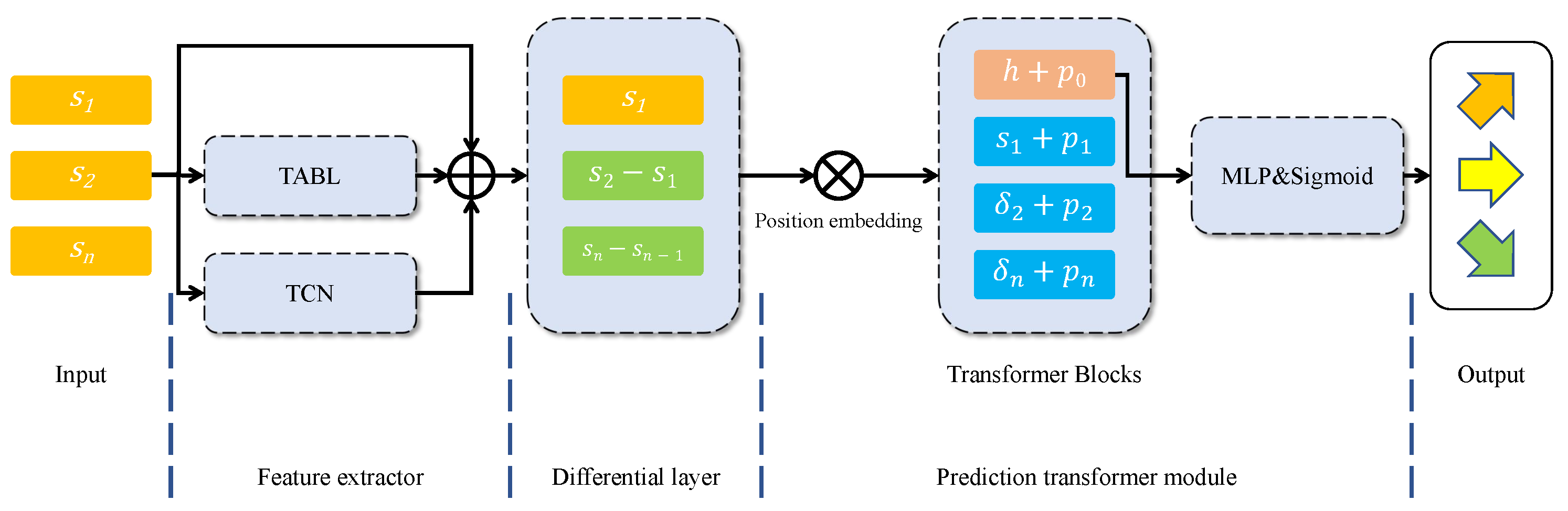
As shown in Figure 1, the proposed model consists of three parts: the feature extractor, the differential layer, and the prediction transformer module. The feature extractor is used to remove the noise in the input data and extract feature vectors, as financial data are notoriously noisy with a low signal-to-noise ratio. The differential layer is developed to scale the feature. This layer calculates the differential of the adjacent vectors and normalizes them, which highlights the difference between adjacent vectors and makes the data more evenly distributed. The prediction transformer module is then used to capture the dependency of the processed features and predict the movement of the shares.

4.1. Feature Extractor

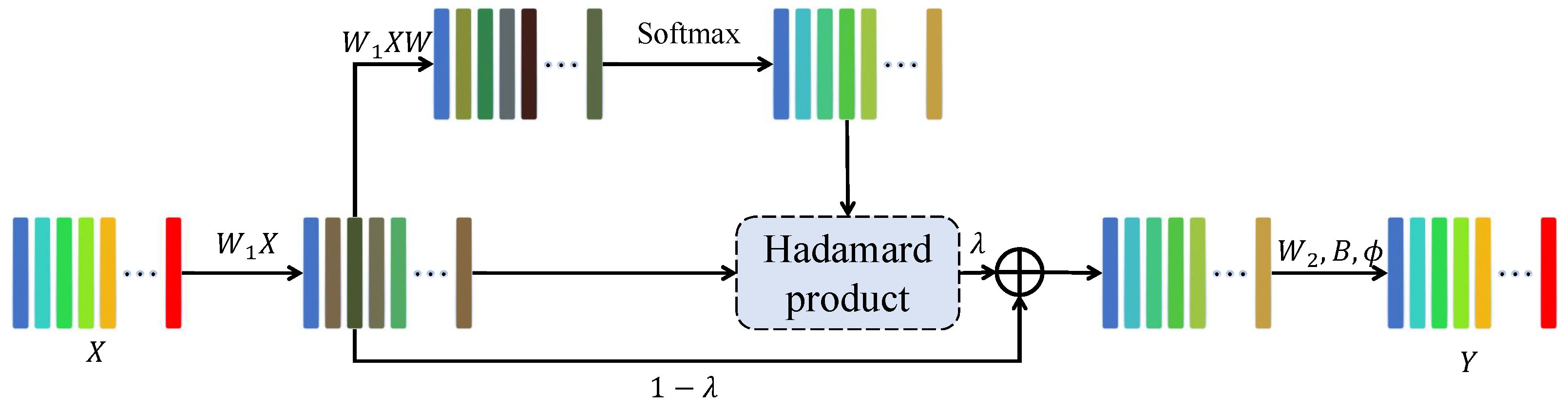
The feature extractor combines the TCN model and the TABL model to extract features and to denoise the data. The TABL model is proposed in [15], and its structure is shown in Figure 2. The formulas are

$$\begin{array}{cc}\hfill & \overline{X}=W_{1}X,\hfill \end{array}$$

(3a)

$$\begin{array}{cc}\hfill & E=\overline{X}W,\hfill \end{array}$$

(3b)

$$\begin{array}{cc}\hfill & {\alpha }_{ij}=\frac{\exp \left(e_{ij}\right)}{{\sum }_{k=1}^T\exp \left(e_{ik}\right)},\hfill \end{array}$$

(3c)

$$\begin{array}{cc}\hfill & \tilde{X}=\lambda (\overline{X}\odot A)+(1-\lambda )\overline{X},\hfill \end{array}$$

(3d)

$$\begin{array}{cc}\hfill & Y=\varphi (\tilde{X}{W}_2+B),\hfill \end{array}$$

(3e)

in which $W_1$, W, $W_2$, B are the learnable parameters; $\overline{X}$, E, and $\tilde{X}$ are intermediate variables; ⊙ denotes the Hadamard product; $\varphi (·)$ denotes a ReLU function [39]; and Y is the final output. The TABL model is characterized by integrating the bilinear projection and the global attention in two dimensions, which improves the model’s interpretability and its capability to capture the global features of the sequence.

In the TABL model, multivariate time series are naturally expressed in terms of two-point tensors, in which the time information is implicitly encoded. The TABL model first learns the weights of the data at different positions on a vector in a two-dimensional tensor, then learns the weights at different times through the attention mechanism. In this way, the resulting vectors in feature tensors contain the information of all other vectors, i.e., each vector is a combination of its information and the global information.

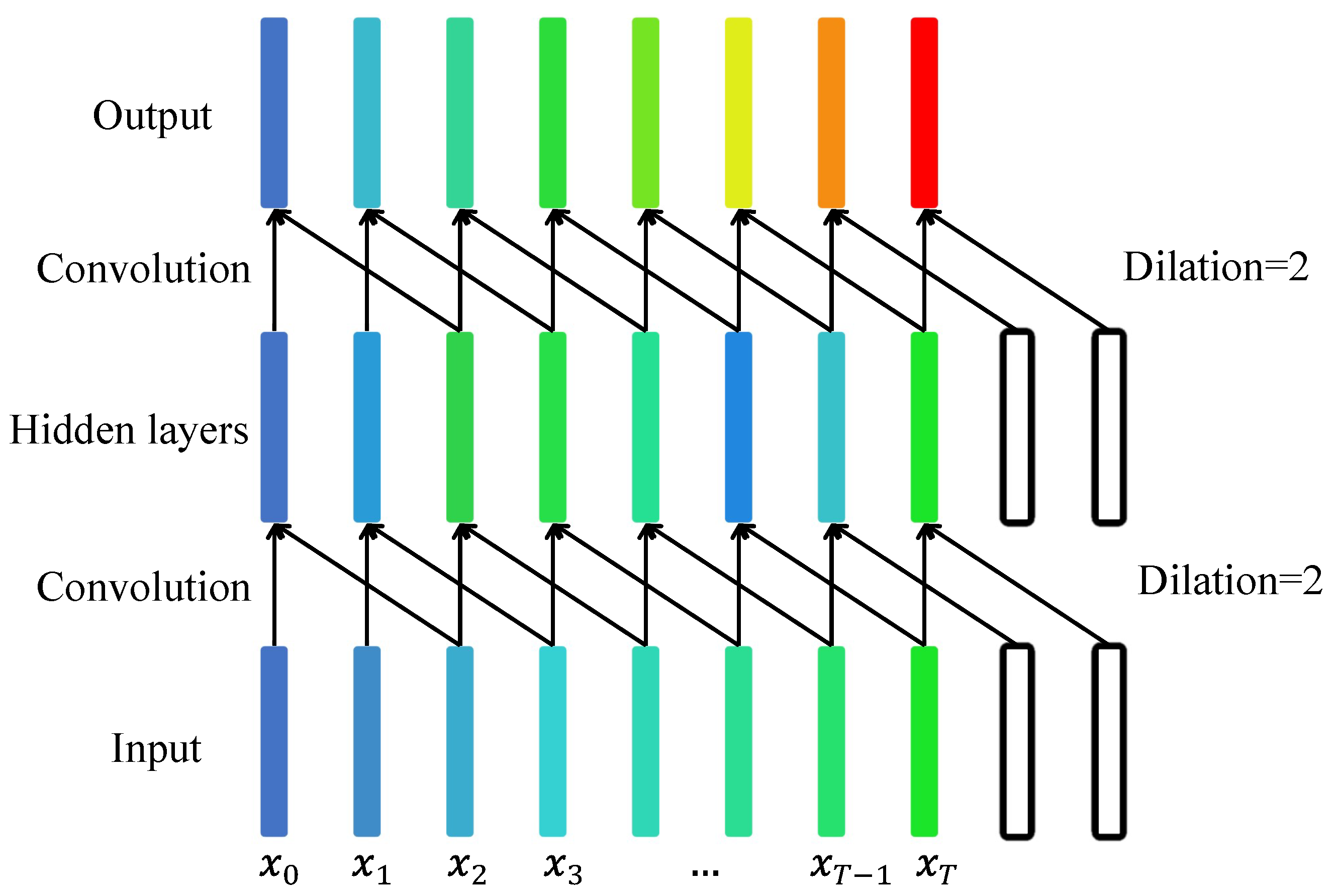
The TCN model is proposed in [14], and its structure is shown in Figure 3; the model combines the idea of dilative convolutions and causal convolutions and uses them to extract the sequence information.

According to [40], the vast majority of orders are canceled. Some of the canceled orders contain a lot of false information and noise. Therefore, it is necessary to denoise the two-dimensional tensor of the time series. A component of the TCN model is a one-dimensional convolution layer with expansion. It can learn the weight of each value in a vector and finally obtain a new value. Therefore, the TCN model can find the local features of the data with the learned weights. As this process continuously flattens the data, the noise is significantly reduced.

The input data are processed with the TABL model and the TCN model, respectively. To obtain a feature vector with identical dimensions, they are then integrated via a residual module. In this way, we obtain the extracted feature vectors with the same dimension.

4.2. Differential Layer

After the feature extractor, each element in the input sequence can be reformulated as a state vector of the corresponding slice. The input sequence can be denoted as $(s_1,s_2,\dots ,s_n)$. Each state vector can be re-represented as $s_i$ by the difference between the two adjacent states $s_i=s_{i-1}+{\delta }_i$. Then, the input sequences are reformulated as $(s_1,s_1+{\delta }_2,s_2+{\delta }_3,\dots ,s_{n-1}+{\delta }_n)$.

It is noted that the LOB data series is composed of high-frequency data. Even the extracted state vectors have small differences between adjacent vectors, i.e., the difference ${\delta }_i$ is negligible in comparison with the state vector $s_i$. However, the difference is what we need to emphasize.

To solve this problem, a differential layer is proposed. In the differential layer, each vector in the input sequence, except the first vector, will be set as a variation of itself and the prior one. In other words, the input sequence can be denoted as $(s_1,s_1+{\delta }_2,s_2+{\delta }_3,\dots ,s_{n-1}+{\delta }_N)$, and after the differential layer, the output sequence is $(s_1,{\delta }_2,{\delta }_3,\dots ,{\delta }_n)$.

In this way, the difference between state vectors is emphasized, which can help the next module, i.e., the prediction transformer module, in improving the capability of capturing patterns. The mathematical justification is given in the next subsection.

4.3. Prediction Transformer Module

In this module, the input vector will be preceded by a classification header and learnable location embedding. Then, the processed input vectors are sent to the multi-head self-attention block for processing. Each vector keeps the same dimension after the attention block with other vectors. Finally, only the classification head is extracted, and the corresponding classification result is outputted through a multi-layer perceptron (MLP) and an activating layer with a sigmoid function.

In the original transformer model, the output sequence has the same length as the input sequence, and each vector in the sequence contains information about the other vectors in the sequence. From a microscopic point of view, each input vector $x_i$ in transformer blocks is first converted into the k, q, and v vectors, i.e.,

$$k={\mathbf{W}}_{\mathbf{k}}{x}_i,q={\mathbf{W}}_{\mathbf{q}}{x}_i,v={\mathbf{W}}_{\mathbf{v}}{x}_i,$$

(4)

where ${\mathbf{W}}_{\mathbf{k}},{\mathbf{W}}_{\mathbf{q}},{\mathbf{W}}_{\mathbf{v}}$ are learnable matrices and are the same for each input vector $x_i$.

Then, its q vector and each k vector are fed into an attention block and a classification function (softmax) to obtain a set of weights $\alpha$. The sum of the products of each $\alpha$ and corresponding v is the output vector to the input vector. The process is

$$\begin{array}{c}{\alpha }_{i,j}=\mathrm{attention}(q_i,k_j),\end{array}$$

(5)

$$\begin{array}{c}(\widehat{{\alpha }_{i,1}},\widehat{{\alpha }_{i,2}},\dots ,\widehat{{\alpha }_{i,n}})=\mathrm{Softmax}({\alpha }_{i,1},{\alpha }_{i,2},\dots ,{\alpha }_{i,n}),\end{array}$$

(6)

$$\begin{array}{c}{y}_i=\sum _{j=1}^n\widehat{{\alpha }_{i,j}}{v}_j,\end{array}$$

(7)

where $y_i$ is the corresponding output of the input $x_i$.

In the ViT [36], however, only the classification header vector is outputted, so the actual output vector is the result of attention between the header vector and other vectors in the sequence. Our model refers to the idea of the ViT and only extracts the head vector. So, the result contains information on all the input vectors and the feature vectors in the whole sequence.

In our model, the input vectors are $(s_1,{\delta }_2,{\delta }_3,\dots ,{\delta }_n)$ delivered from the differential layer. A learnable classification header vector h and the learnable position embeddings $(p_h,p_1,p_2,\dots ,p_n)$ will firstly be added to the input series, and the input series becomes $(h+p_h,s_1+p_1,{\delta }_2+p_2,{\delta }_3+p_3,\dots ,{\delta }_n+p_n)$. Then, the input series is fed into a multi-head attention block, and only the output of the header vector will be reserved.

For simplicity, the input series $(h+p_h,s_1+p_1,{\delta }_2+p_2,{\delta }_3+p_3,\dots ,{\delta }_n+p_n)$ is denoted as $(x_h,x_1,x_2,\dots ,x_n)$, and the output is denoted as $y_h$. According to [12], the output after the transformer blocks with a classification header can be denoted as

$$y_h=\sum _{i=1}^n\mathrm{Softmax}\left(\mathrm{attention}(q_{s_h},k_{x_i})\right)v_{x_i},$$

(8)

$$\mathrm{attention}(q_{s_h},k_{x_i})=q_{s_h}{k}_{x_i}/\sqrt{d},$$

(9)

where $q_{s_h}$ is the query vector of the classification header $s_h$, and $k_{x_i}$ and $v_{x_i}$ are the key vector and value vector of each input vector $x_i$. The attention function can be formulated as the product of two vectors, and d is the dimension of the two vectors. Finally, the vector $y_h$ will be fed into an MLP and an activating layer with a sigmoid function, and the prediction of the stock movement is made.

4.4. Analysis of the Differential Layer and Prediction Transformer Module

Now we will show how the differential layer helps in this process. According to research, stock data is non-stationary [34], meaning that certain statistical indicators of stock data change over time, rendering them difficult to predict. Typically in research, stock data are either original or normalized; however, normalization alone cannot eliminate the non-stationarity of the data. Instead, difference operation can effectively remove this non-stationarity [16].

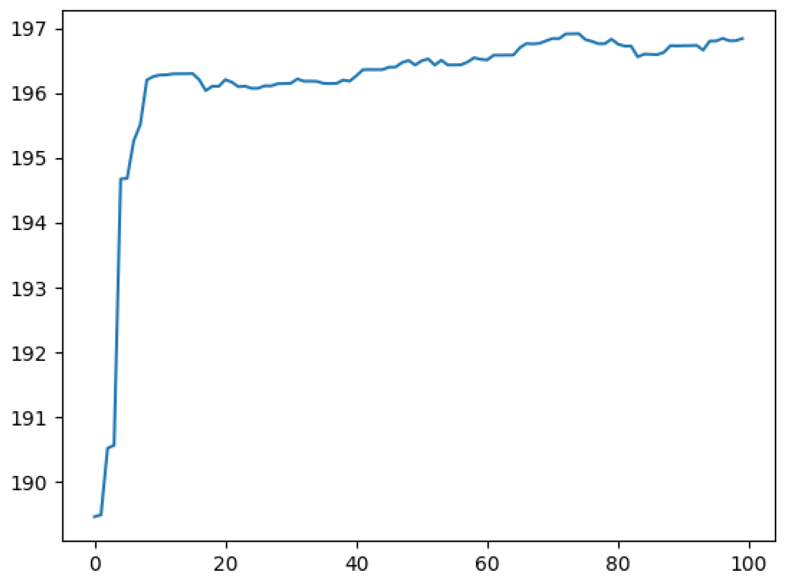
The Figure 4 and Figure 5 depict the L2 norm curves of the original input data and that of the feature-extracted data. It is evident that the former exhibits instability, while the latter, though improved by multiple feature-extraction modules, still displays a discernible trend.

We performed unit root tests on the data. The unit root test is an objective method to determine whether a difference operation is needed [16]. This statistical hypothesis test for stationarity is used to determine whether a difference operation is needed to make the data more stationary. Finally, it is found that only 6% of the original data can be identified as stationary, while 82.2% of the data after the feature-extraction module can be identified as stationary. However, after the differential layer, 98.3% of the data were considered stationary. This shows that the differential layer indeed makes the overall data more stable and thus improves the performance of the model.

Now, let us attempt to analyze this problem mathematically. We first focus on the situation without the differential layer. In this case, the input vectors will become $(h+p_h,s_1+p_1,s_2+p_2,s_3+p_3,\dots ,s_n+p_n)$, and the coefficient after the attention block is

$$\mathrm{attention}(q_{s_h},k_{x_i})\propto q_{s_h}{k}_{x_i}=q_{s_h}{\mathbf{W}}_{\mathbf{k}}(s_i+p_i),$$

(10)

where $q_{s_h}$ and ${\mathbf{W}}_{\mathbf{k}}$ are learnable variables; hence, their product $q_{s_h}{\mathbf{W}}_{\mathbf{k}}$ can be denoted as one coefficient vector c instead. According to [36,41], the attention block is the main structure to capture the patterns of data. So, we focus on the attention block and simplify the attention function $\mathrm{attention}(q_{s_h},k_{x_i})$ in Equation (10) as $A_i$, i.e.,

$$A_i=c{s}_i+c{p}_i=c(s_i+p_i).$$

(11)

Note that c is irrelevant to the input sequence and position of $s_i$. In addition, the position embedding $p_i$ only depends on the position and adapts its scale to $s_i$. Define the difference between $A_i$ and $A_{i-1}$ as ${\Delta }_i$:

$${\Delta }_i=A_i-A_{i-1}=c({\delta }_i+p_i-p_{i-1})\approx c(p_i-p_{i-1}).$$

(12)

It is noted that the input LOB data are high-frequency data, and the difference between two adjacent state vectors ${\delta }_i$ is negligible. Hence, the difference ${\Delta }_i$ defined in Equation (12) is mainly correlated with the position embeddings $p_i$ and $p_{i-1}$, which results in the attention block mainly observing the patterns of the position embeddings but not the patterns of the state vectors. However, the latter is what we need to emphasize.

Then, we analyze the situation with the differential layer. The differential layer differentiates the extracted features and reformulates the input vectors as $(h+p_h,s_1+p_1,{\delta }_2+p_2,{\delta }_3+p_3,\dots ,{\delta }_n+p_n)$. According to Equations (11) and (12), $A_i$ and ${\Delta }_i$ can be reformulated as $A_i^{\prime }$ and ${\Delta }_i^{\prime }$:

$$A_i^{\prime }=h{\delta }_i+h{p}_i=h({\delta }_i+p_i),{\Delta }_i^{\prime }=h({\delta }_i-{\delta }_{i-1}+p_i-p_{i-1}).$$

(13)

Since the position embedding $p_i$ will adapt to ${\delta }_i$, ${\delta }_i$ cannot be neglected in Equation (13). The new difference ${\Delta }_i^{\prime }$ depends not only on the position embeddings $p_i$ and $p_{i-1}$ but also on the changes of states ${\delta }_i$ and ${\delta }_{i-1}$. Such a block highlights the variance in feature series and facilitates the resolution of the network.

5. Experimental Design

5.1. Experiment on Benchmark Dataset

FI-2010 is a public benchmark dataset that collects normalized time series data of five stocks on the Nasdaq Nordic Stock Market for ten consecutive days [22]. It is a normalized dataset including about 4 million time series collected with 10 events in a slice. The provided data are z-score normalized and labeled directly to keep the original data confidential. The original dataset contains 144 features, where we only adopt the 40 features that the ordinary LOB data contain, namely, numbers of orders and prices of ask orders and bid orders. Several baseline methods are provided in the dataset. In most work that considered these data, the model uses information from the past 100 slices to forecast the future movement direction. The prediction horizons are 10, 20, 50, and 100 events, i.e., 1, 2, 5, and 10 slices, as 1 slice contains the data of 10 events. Thus, in our experiments, the input data are $X\in {\mathbb{R}}^{40\times 100}$, the number of slices used in the prediction is $T=100$, and the horizons are $k=10,20,50,100$.

In the experiment with FI-2010, the data from the first seven days are selected as the training and verification sets, and the data from the last three days as the chosen test set. We reproduced these models based on the paper and ensured that all experiments were conducted under identical conditions, so we can make a fair comparison in this way. These models are support vector machine (SVM) [25], MLP [25], CNN [42], LSTM [3], CNN-LSTM [43], TABL [15], DeepLOB [5,38], and DeepLOB-Attention [5]. Among them, the TABL model is a two-layer stack of TABL modules with the module structure described above. The DeepLOB model consists of a CNN and LSTM structure, with a unique Inception Module added between the CNN and LSTM layers. The Deeplob-attention model builds upon the DeepLOB model by incorporating Seq2Seq and Attention models into its output.

First, we test our complete model with different horizons with the experimental set-ups used in the DeepLOB [38]. Then, the prediction accuracy, precision, recovery rate, and F1 score are compared with the same evaluation indices of other models. To show that the proposed differential layer is adequate, we conducted an ablation study. We compare the results and evaluate the contribution of the differential layer by removing it without changing other settings. Furthermore we conducted a comprehensive ablation study by separately removing the feature extractor and the prediction transformer module from the model.

To conduct a comprehensive evaluation of our model, we present a new dataset called the dataset from Huang [44], and perform a series of experiments. It is worth noting that, due to the distinct data processing from the evaluation index from FI2010, we solely utilize the original data provided by it while maintaining consistency in terms of data processing, labeling method, and evaluation index with FI2010 for DTNN and DeepLOB testing.

5.2. Experiment on Real Stock Data

To demonstrate the practicality and universality of our model, we select actual Chinese stock data to assess its performance.

Two groups are used in the experiment: The first group uses a similar configuration as the FI-2010 experiment, i.e., ten stocks are selected, and the data of 7 days (from 1 November 2021 to 9 November 2021) are used for training and verification (80% of data are used for training, and 20% of the data are used for verification), and the data of the next three days (from 10 November 2021 to 12 November 2021) are used for testing. The second group takes a more general approach by training data for ten days (from 1 November 2021 to 12 November 2021) from 100 stocks and testing data for the next five days (from 15 November 2021 to 19 November 2021) from another five stocks.

We merge all the data used for training and normalize them via z-score during preprocessing. The scale from the training data is then used to normalize the test data.

6. Results

Table 1. Experimental results for the FI-2010 Dataset (k = 10).

Model	Accuracy %	Precision %	Recall %	F1 %
SVM [25]	70.83	69.22	70.83	59.07
MLP [25]	72.63	70.54	72.63	66.26
CNN [42]	76.79	74.69	76.79	73.84
LSTM [25]	74.07	72.40	74.07	67.90
CNN-LSTM [43]	76.52	74.30	76.52	74.50
TABL [15]	84.70	76.95	78.44	77.63
DeepLOB [38]	84.74	84.00	84.74	83.40
DeepLOB-Attention [5]	83.28	82.50	83.28	82.37
DTNN	87.69	87.92	87.69	86.92

,

Table 2. Experimental results for the FI-2010 Dataset (k = 20).

Model	Accuracy %	Precision %	Recall %	F1 %
SVM [25]	62.25	57.15	62.25	49.57
MLP [25]	62.58	57.69	62.58	57.23
CNN [42]	67.93	65.21	67.93	64.97
LSTM [25]	63.46	58.81	63.46	57.68
CNN-LSTM [43]	66.93	64.33	66.93	64.78
TABL [15]	73.74	67.18	66.94	66.93
DeepLOB [38]	74.85	74.06	74.85	72.82
DeepLOB-Attention [5]	75.25	74.31	75.25	73.73
DTNN	78.66	78.44	78.66	77.14

,

Table 3. Experimental results for the FI-2010 Dataset (k = 50).

Model	Accuracy %	Precision %	Recall %	F1 %
SVM [25]	47.54	48.21	47.54	47.79
MLP [25]	53.24	52.36	53.24	51.74
CNN [42]	66.76	66.62	66.76	66.65
LSTM [25]	58.12	57.32	58.12	57.25
CNN-LSTM [43]	66.50	66.42	66.50	66.45
TABL [15]	79.87	79.05	77.04	78.44
DeepLOB [38]	80.51	80.38	80.51	80.35
DeepLOB-Attention [5]	79.49	79.51	79.49	79.38
DTNN	88.00	88.19	88.00	87.94

and

Table 4. Experimental results for the FI-2010 Dataset (k = 100).

Model	Accuracy %	Precision %	Recall %	F1 %
SVM [25]	43.60	48.96	43.60	38.05
MLP [25]	49.81	52.04	49.81	47.03
CNN [42]	65.22	66.03	65.22	65.22
LSTM [25]	55.94	57.37	55.94	55.64
CNN-LSTM [43]	66.30	67.18	66.30	66.41
DeepLOB [5]	76.72	76.85	76.72	76.76
DeepLOB-Attention [5]	81.45	81.62	81.45	81.49
DTNN	92.53	92.56	92.53	92.53

show the results of the experiments on the dataset FI-2010, where the horizons are 10, 20, 50, and 100, correspondingly. The metrics used for evaluating the results include accuracy, precision, recall, and F1 score. Following the suggestion in [22], we focus more on the F1 score performance since the data distribution of the FI-2010 dataset is not balanced enough. For comparison, we also present the results from other existing methods, including support vector machine (SVM) [25], MLP [25], CNN [42], LSTM [3], CNN-LSTM [43], TABL [15], DeepLOB [5,38], and DeepLOB-Attention [5]. The data differ from those presented in the original paper due to the replication experiment. The highest scores have been labeled in bold.

It can be seen from the tables that our model leads to a significant improvement on all horizons. When the horizons are 10, 20, and 50, the F1 scores are 86.92%, 77.14%, and 87.94%, respectively, which is 3.52%, 4.32%, and 7.59% higher than the F1 scores of DeepLOB and 4.55%, 3.41%, and 8.56% higher than DeepLOB-Attention. When the horizon is 100, there are few works to compare with since only [5,42] reported experimental results under this horizon, and we achieve an F1 score of 92.53%, which is 11.04% higher than the DeepLOB-Attention. In short, our model outperforms other comparative state-of-the-art methods in terms of F1 score.

Table 5. Experimental results for the dataset from Huang.

Model	Horizon	Accuracy %	Precision %	Recall %	F1 %
DeepLOB	20	99.05	98.11	99.05	98.58
	50	97.93	95.91	97.93	96.91
	100	96.44	93.02	96.44	94.70
DTNN	20	99.05	98.11	99.05	98.58
	50	97.93	95.91	97.93	96.91
	100	96.44	93.68	96.44	94.78

presents the results of DTNN and DeepLOB on the dataset from Huang. Despite the suboptimal quality of this dataset, which is primarily labeled as “unchanged”, causing significant challenges for model performance, DeepLOB still outperforms DTNN by a small margin in terms of F1 score due to its ability to recognize low-frequency labels.

As for the ablation study, it can be found from

Table 6. Experimental results of the ablation study.

DTNN	Horizon	Accuracy %	Precision %	Recall %	F1 %
Without Differential layer	10	80.44	79.13	80.44	78.88
	20	68.19	66.52	68.19	67.00
	50	70.80	71.70	70.80	71.05
	100	70.38	71.12	70.38	70.39
Without Feature Extractor	10	80.79	79.67	80.79	79.04
	20	70.25	68.29	70.25	68.19
	50	55.94	56.82	55.94	56.33
	100	67.77	68.78	67.77	67.84
Without Transformer Module	10	70.69	49.97	70.69	58.55
	20	77.62	78.65	77.62	75.57
	50	78.80	79.17	78.80	78.67
	100	61.23	61.59	61.23	58.12
Complete DTNN	10	87.69	87.92	87.69	86.92
	20	78.66	78.44	78.66	77.14
	50	88.00	88.19	88.00	87.94
	100	92.53	92.56	92.53	92.53

that the model with the differential layer performs much better than the model without the differential layer. For comparison, the F1 scores of the models without the differential layer under each horizon are only 78.88%, 67.00%, 71.05%, and 70.39%, which are decreases of 8.04%, 10.41%, 16.89%, and 22.14%. So, we conclude that the differential layer can significantly improve the model’s effectiveness. In addition, after the exclusion of the feature extractor and the prediction transformer module, a significant reduction in F1 score is also observed.

The results of the experiments with real data are shown in

Table 7. Experimental results with real data (Group 1).

Horizon	Accuracy %	Precision %	Recall %	F1 %
10	90.37	81.66	90.37	85.79
20	84.65	71.66	84.65	77.62
50	74.33	67.79	74.33	66.09
100	65.56	61.81	65.56	62.08

and

Table 8. Experimental results with real data (Group 2).

Horizon	Accuracy %	Precision %	Recall %	F1 %
10	88.10	77.61	88.10	82.53
20	82.07	67.35	82.07	73.98
50	70.31	65.89	70.31	66.60
100	61.49	58.26	61.49	59.10

. In the first group of experimental configurations, we obtained F1 scores of 85.79%, 77.62%, 66.09%, and 62.08% under each prediction horizon. In the second group, we obtained F1 scores of 82.53%, 73.98%, 66.60%, and 59.10%. The experimental results of the second group are lower than those of the first group because the training patterns of the second group cover a longer period, and the stocks used for training differ from those used for testing. Hence, the accuracy and F1 score seem lower than the first group’s. However, even for the largest time horizon in the second group, the F1 score can still be about 60%, which is enough to show that our model has practical significance.

7. Conclusions

This paper proposes a transformer-based model, dubbed DTNN, to predict stock price movement with LOB data. A differential layer is developed to improve the prediction capability of the model. The experimental results show that our model outperforms other comparative state-of-the-art methods in accuracy, precision, recall, and F1 scores. The experimental results also validate the potential and feasibility of utilizing the transformer model for stock prediction. Furthermore, ablation study confirmed the effectiveness of our proposed differential layer.

In future work, we hope our model can serve as a crucial tool for guiding business strategies in the realm of high-frequency trading. Firstly, we plan to conduct further research to enhance the model’s predictive accuracy beyond mere trends and towards stock change magnitude, thereby accommodating more intricate investment strategies. Additionally, we will explore the application of this model in other sequences with similar characteristics—specifically those similar to high-frequency trading and low signal-to-noise ratios.

During the experiment, we also identified some limitations of our model. Firstly, the model is a trend predictor and can only forecast direction rather than specific proportions. However, businesses require models that are precise enough to predict changes in magnitude, so that they can navigate complex asset allocation and risk hedging. If only the direction can be predicted, the investment strategy will be severely limited. Moreover, the model itself is designed for high-frequency stock-trading scenarios. If the input sequence lacks non-stationarity and low signal-to-noise ratio characteristics, DTNN’s advantage over other models is not obvious obvious.