Article

A Customized ECA-CRNN Model for Emotion Recognition Based on EEG Signals

School of Physics, Liaoning University, Shenyang 110036, China
*
Author to whom correspondence should be addressed.
Electronics 2023, 12(13), 2900; https://doi.org/10.3390/electronics12132900
Submission received: 19 May 2023 / Revised: 26 June 2023 / Accepted: 29 June 2023 / Published: 1 July 2023
(This article belongs to the Special Issue New Machine Learning Technologies for Biomedical Applications)

Abstract

:
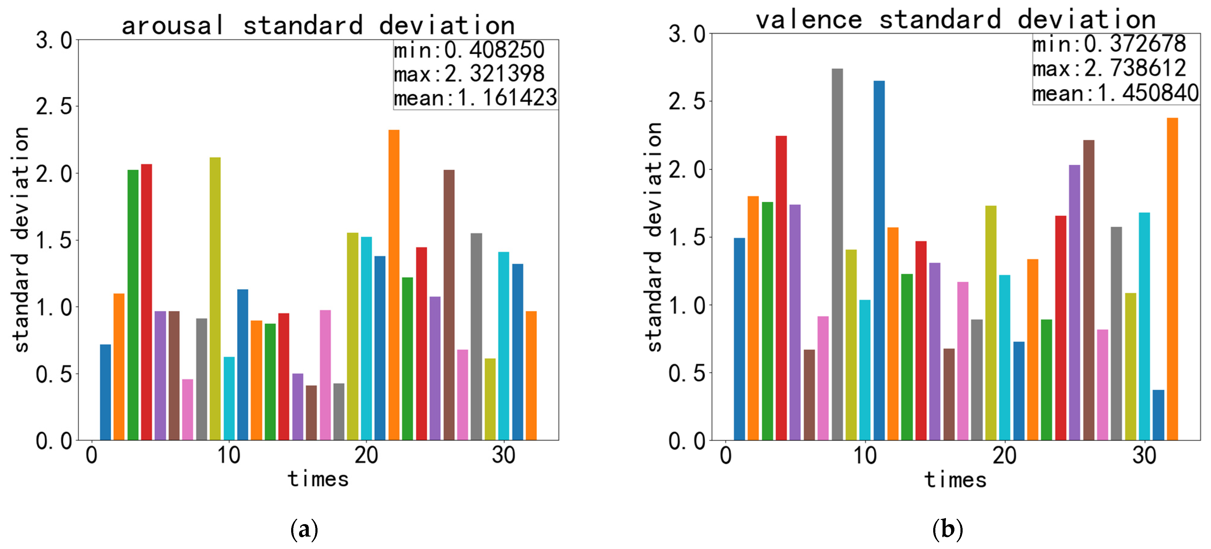
Electroencephalogram (EEG) signals are electrical signals generated by changes in brain potential. As a significant physiological signal, EEG signals have been applied in various fields, including emotion recognition. However, current deep learning methods based on EEG signals for emotion recognition lack consideration of important aspects and comprehensive analysis of feature extraction interactions. In this paper, we propose a novel model named ECA-CRNN for emotion recognition using EEG signals. Our model integrates the efficient channel attention (ECA-Net) module into our modified combination of a customized convolutional neural network (CNN) and gated circulation unit (GRU), which enables more comprehensive feature extraction, enhances the internal relationship between frequency bands and improves recognition performance. Additionally, we utilize four-dimensional data as input to our model, comprising temporal, spatial and frequency information. The test on the DEAP dataset demonstrates that it enhances the recognition accuracy of EEG signals in both arousal and valence to 95.70% and 95.33%, respectively, while also reducing the standard deviation during five-fold cross-validation to 1.16 and 1.45 for arousal and valence, respectively, surpassing most methods.

1. Introduction

The brain is comprised of telencephalon and diencephalon, with the former being responsible for regulating behavior, generating affective states, as well as executing cognitive functions. The diencephalon is divided into the thalamus and hypothalamus [1], which are independently responsible for directing movement, transmitting sensation and maintaining emotional stability. Due to the intricate structure and multifaceted functions of the brain, the conveyed messages it transmits are of the utmost significance. As a form of information produced by the brain, as well as an intuitive and subjective response exhibited by individuals towards external stimuli, emotion is significant to the analysis of people’s mental activities and the detection of mental conditions [2]. Therefore, emotion recognition is a valuable approach for assessing individuals’ mental well-being. When it comes to recognizing emotions, relying solely on external expressions may not always provide sufficient information for accurate judgments. Deep learning methods utilizing EEG signals could effectively solve this kind of problem. In recent years, deep learning has advanced rapidly and has been widely used in image recognition, automatic speech recognition (ASR), character recognition, physiological signal processing and other fields [3]. As a subfield of artificial intelligence within machine learning, compared to traditional machine learning, deep learning does not require manually extracting features and it has higher accuracy and faster recognition speed. Using various deep learning networks and related variants for emotion recognition through EEG signals has gradually become the mainstream technique.
There are various approaches to emotion recognition. The literature [4] could improve that CNN is better than traditional machine learning. The literature [4] compared shallow machine learning such as bagging tree (BT) and support vector machine (SVM) with CNN on the DEAP dataset. The results indicate that BT has the best performance among shallow machine learning methods but CNN achieves a recognition accuracy that surpasses BT classifiers by 3.58% in valence and 3.29% in arousal. Although CNN has the capability of extracting more features, both the processing of raw data and the architecture of CNN need improvement. The literature [5] proposed a three-dimensional convolutional neural network called EmotioNet and raw data from the DEAP dataset was used as input to CNN for the first time, which solved issues related to the covariance shift and the unreliability of emotional ground truth. Their classification results achieved 73.3% and 72.1% accuracy for arousal and valence, respectively, for the DEAP dataset. The literature [6] proposed a continuous convolutional neural network utilizing baseline signals. They constructed a 3D EEG cube as the input and they achieved recognition accuracies of 90.24% and 89.45% for arousal and valence, respectively, for the DEAP dataset. The literature [7] proposed a hierarchical CNN model that attains a recognition accuracy of 88.60% for the SEED dataset. It demonstrated that improved CNN has an excellent performance in emotion recognition but CNN is limited to extracting features solely in the spatial and frequency domains. The literature [8] proposed a model combining CNN and LSTM and compared the performance of a single CNN with a CNN and LSTM for the DEAP dataset. The results indicate that the accurate extraction rate of raw data reached 90.12% for CNN alone, while the combination of CNN and LSTM achieved an even higher accuracy rate of 94.17%. This suggests that the fusion of CNN and LSTM is superior to using only a single CNN in feature extraction. The literature [9] considered utilizing baseline signals and a preprocessing method of converting the chain-like EEG sequences into a 2D-like frame sequence with a combination of CNN and LSTM. The results yielded an average accuracy rate of 90.80% for valence and 91.03% for arousal for the DEAP dataset. The literature [10] proposed an ensemble three-branch model, which is composed of a CNN, LSTM and the fusion of CNN and LSTM. This model achieved a recognition accuracy of 97.16 ± 1.08% for the SEED dataset and achieved a recognition accuracy of 65.00 ± 3.57% for the DEAP dataset. Its contribution lies in not only incorporating the DE feature but also utilizing the three branches to perform distinct tasks that are significant for learning. The literature [11] conducted a performance comparison between CNN-GRU and CNN-LSTM on the DEAP dataset under equal conditions. The results indicate that both models exhibit similar recognition accuracy, but due to its lightweight construction, CNN-GRU achieves a faster processing speed. This highlights the superior efficiency of GRU over LSTM. The literature [12] proposed several different methods including 2D CNN, 3D CNN, CRNN and 4D CRNN to prove the superiority of multidimensional features. Among them, CNN extracts spatial and frequency features, CRNN extracts temporal and spatial features, while 4D-CRNN extracts temporal, spatial and frequency features. The 3D CNN model from the literature [12] achieved an average accuracy rate of 91.03 ± 2.49% for valence and 92.16 ± 2.78% for arousal for the DEAP dataset. Its model is the first half of the 4D-CRNN and it takes a 2D map and DE features as input. The 4D-CRNN model, which consists of CNN and LSTM, outperforms the other models. It utilizes a temporal sequence, 2D map and differential entropy (DE) features that are enhanced by frequency to construct four-dimensional (4D) features. The recognition accuracy for valence and arousal for the DEAP dataset reached 94.22% and 94.58%, respectively.
Considering all existing methods, this paper incorporates their advantages while retaining the original concept of combining CNN and sequential network GRU [13]. The CNN network is utilized to extract spatial and frequency features, while the GRU extracts temporal features. But the difference is that we change the structure of CNN and we incorporate the efficient channel attention module to facilitate the interaction between frequency bands. Our method has been tested on the DEAP dataset and compared against other methods, demonstrating superior feature extraction capabilities that enhance valence and arousal recognition accuracy while significantly reducing errors across all test groups. The main contributions to this paper are as follows:
  • A new network named the ECA-CRNN model is proposed, which incorporates the Efficient Channel Attention Module for the first time to enhance emotion recognition using EEG signals;
  • The ECA-CRNN model employs the attention mechanism for emotion recognition with EEG signals, originally used in image recognition, demonstrating the broad application and conveniences of ECA in enhancing the relationship between channels;
  • The initial EEG signal is converted into a four-dimensional input dataset comprising temporal, spatial and frequency information. The customized CNN extracts spatial and DE frequency features, while GRU extracts temporal features. This comprehensive feature extraction approach results in more accurate emotion recognition outcomes;
  • The ECA-CRNN model demonstrated superior performance on the DEAP dataset, exhibiting the lowest standard deviation and maintaining a relatively high recognition accuracy compared to some other methods we have tested.
This paper is structured as follows: Section 2 provides an introduction to the DEAP dataset, outlines the methodology for extracting temporal, frequency and spatial features, as well as a detailed description of the ECA-CRNN model’s architecture; Section 3 provides the comprehensive experimental data and comparisons with several methods we have verified; Section 4 analyzes and discusses the experimental results; Section 5 concludes our work.

2. ECA-CRNN’s Model Constructing

2.1. DEAP Dataset

The database for emotion analysis using physiological signals (DEAP) [14] was developed by the Queen Mary University of London, the University of Twente, the University of Geneva and others, which obtained EEG data from 16 male and 16 female subjects. During the experimental period, every experimental subject was required to watch 40 one-minute music videos, resulting in different moods among subjects. The sponsors recorded subjects’ physiological variations, which were captured at a frequency of 512 Hz across 40 channels, including the peripheral physiological signals and EEG signals. Additionally, the facial expressions of 22 subjects were also recorded during video viewing. After the experiment, each subject’s data recorded by the sponsors were collated, which included a baseline recording of three seconds when switching videos and an experimental recording lasting sixty seconds while watching. Lastly, based on the video they just viewed, the subjects provided their subjective ratings for four evaluation criteria: valence, arousal, dominance and liking [15,16,17,18,19].
In the course of acquiring EEG signals via the headset, the placement of EEG electrodes follows the 10–20 system methodology [20,21,22]. The 10–20 system electrode placement method is a standardized approach prescribed by the International Electroencephalogram Society, which enables precise capture of human EEG signals and facilitates sleep condition research. In this specific methodology, the locations of different channels are determined based on 10% or 20% of the total length of the anterior and posterior aspects of the cranium, the upper part of the human brain is compartmentalized into different channels, which are ultimately identified and labeled with English abbreviations and numerical designations based on their respective locations.
Figure 1 illustrates the channel diagram of the 10–20 system. The combinations of letters and numbers in Figure 1 represent different electrical brain channels.
Upon conclusion of the experiment, a total of 32 distinct data files were generated for analysis and learning based on the scores obtained from 32 subjects. The sampling frequency of the dataset was reduced to 128 Hz after down-sampling. Based on the duration of EEG signal acquisition and the electrode placement for signal acquisition, each subject’s data file comprised a 40 × 40 × 8064 data matrix representing 8064-length data across 40 channels of 40 videos, as well as a 40 × 4 label matrix that denotes four scoring indicators for each of the 40 videos.

2.2. Method of Feature Extraction

According to the characteristics of the DEAP dataset and in order to obtain EEG information more accurately, our main approach to feature extraction involved converting the original DEAP dataset into the input data, which contains multiple dimensions of information first. We then extracted the frequency and spatial features using a customized CNN, as well as temporal features using GRU [23,24,25]. The process of feature extraction can be divided into three parts: temporal feature, frequency feature and spatial feature.

2.2.1. Temporal Feature

Since the DEAP dataset consists of fixed-duration data fragments, temporal information can be easily extracted and identified from its data matrix. To achieve this, the original signal was divided into specific time segments and a time sequence forecasting method such as GRU was employed to extract hidden details within each fragment [26].

2.2.2. Frequency Feature

EEG signals can be divided into 5 different frequency bands: delta waves (1–4 Hz) appear during sleep and anesthesia and are used to monitor sleep status; theta waves (4–7 Hz) increase under conditions of fatigue; alpha waves (7–12 Hz) appear when the overall state of a human being is calm and stable; beta waves (12–30 Hz) appear when executing motion commands and observing others’ movements; and gamma waves (30–50 Hz) occur during periods of high concentration. For emotion recognition, the brain waves in the theta, alpha, beta and gamma bands are the most relevant and suitable for data analysis [27,28]. Therefore, it was appropriate to apply a 4–50 Hz bandpass filter to the original DEAP dataset in order to extract these four frequency bands. Additionally, prior to decomposing the brainwaves by type, basic noise elimination processing can be implemented.
In order to achieve a more effective classification and uncover deeper insights from the dataset, it was considered whether to further divide the frequency bands and extract frequency features based on each temporal segment (as described in Section 2.2.1). Moreover, the literature [29] has demonstrated that differential entropy (DE) features outperform original frequency features in emotion recognition. Therefore, we opted to utilize the DE features as frequency features. Differential entropy in this paper refers to the measure of information entropy, which quantifies the amount of information that can be transmitted and is used to describe the probability distribution of random events. The greater the amount of remaining information, the higher the level of information entropy and, thus, the lower the likelihood for a random event to occur. Entropy also represents the stochastic component of a random event. Information entropy is also known as Shannon entropy. The formula for calculating Shannon entropy of the discrete variable X is as follows:
H Δ x ( X ) = i = f ( x i Δ x ) log ( f ( x i ) Δ x )
As a generalization of Shannon entropy, differential entropy is utilized to quantify the overall uncertainty in the probability distribution of continuous random variables. Therefore, the DE features contain more information than the original frequency features [30]. Utilizing DE features results in better recognition performance and more accurate outcomes. The differential entropy calculation formula for the continuous random variable X is as follows:
h ( X ) = a b f ( x ) log ( f ( x ) ) d x
f ( x ) is the density function, a and b are the lower limit and upper limit of x .

2.2.3. Spatial Feature

Regarding spatial dimension, the EEG signals transmitted by the human body at each electrode position on the scalp exhibit subtle disparities. Therefore, according to the idea of the 10–20 electrode system, decomposition and analysis are conducted based on different electrode positions. In order to facilitate the description of the spatial features, the overhead space was constructed as an h × w matrix according to the electrode placement. We opted to partition the overhead space into an 8 × 9 grid akin to a compact map instead of a sparse map [7], with unoccupied positions denoted by 0, as illustrated below:
[ 0 0 AF 3 FP 1 FPZ FP 2 AF 4 0 0 F 7 F 5 F 3 F 1 FZ F 2 F 4 F 6 F 8 FT 7 FC 5 FC 3 FC 1 FCZ FC 2 FC 4 FC 6 FT 8 T 7 C 5 C 3 C 1 CZ C 2 C 4 C 6 T 8 TP 7 CP 5 CP 3 CP 1 CPZ CP 2 CP 4 CP 6 TP 8 P 7 P 5 P 3 P 1 PZ P 2 P 4 P 6 P 8 PO 7 PO 5 PO 3 PO 1 POZ PO 2 PO 4 PO 6 PO 8 0 0 CB 1 O 1 OZ O 2 CB 2 0 0 ]    
Only 32 electrode positions were utilized in the DEAP dataset. Therefore, the real spatial position matrix employed in our experiment is presented below:
[ 0 0 AF 3 FP 1 0 FP 2 AF 4 0 0 F 7 0 F 3 0 FZ 0 F 4 0 F 8 0 FC 5 0 FC 1 0 FC 2 0 FC 6 0 T 7 0 C 3 0 CZ 0 C 4 0 T 8 0 CP 5 0 CP 1 0 CP 2 0 CP 6 0 P 7 0 P 3 0 PZ 0 P 4 0 P 8 0 0 PO 3 0 0 0 PO 4 0 0 0 0 0 O 1 OZ O 2 0 0 0 ]    
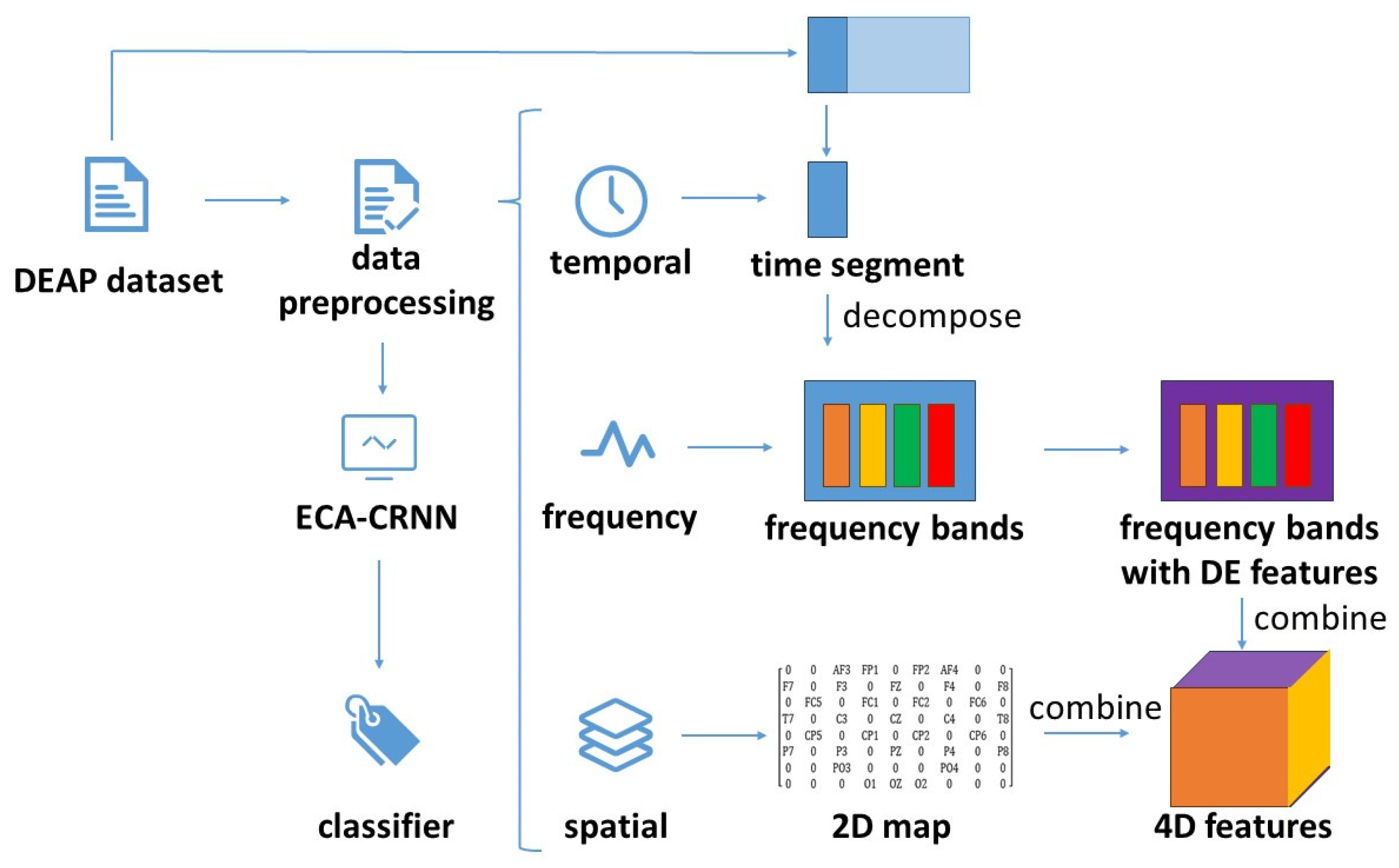
Due to the DEAP dataset being collected based on brain electrical channels, the compact map could establish a correlation with the processed data of Section 2.2.2. By integrating temporal, spatial and frequency domain dimensions, the processed dataset could be fed into the network for feature extraction in their respective dimensions. The diagram of data processing is shown in Figure 2:
The final 4D feature was obtained by integrating temporal segments, the DE feature was transformed from four frequency bands and 2D position information. To enhance the efficacy of the feature extraction, it was crucial to consider spatial and frequency dimensions as well as their interrelation. Therefore, we propose a method that combines space and frequency together and represents them in an image form. The four frequency bands could be seen as color channels of images and the 2D map representing spatial information could be seen as pixels of images. By utilizing attention mechanisms for the feature extraction similar to those used in image recognition, temporal features could then be explored using GRU models.

2.3. Efficient Channel Attention Module

The attention mechanism is a strategy based on machine vision that involves focusing on specific areas of an image during recognition while disregarding irrelevant information to enhance overall performance. Since the input for image recognition models consists of multidimensional image data, if the input data of emotion recognition meets the size and dimension requirements, it can be considered to be image data in theory.
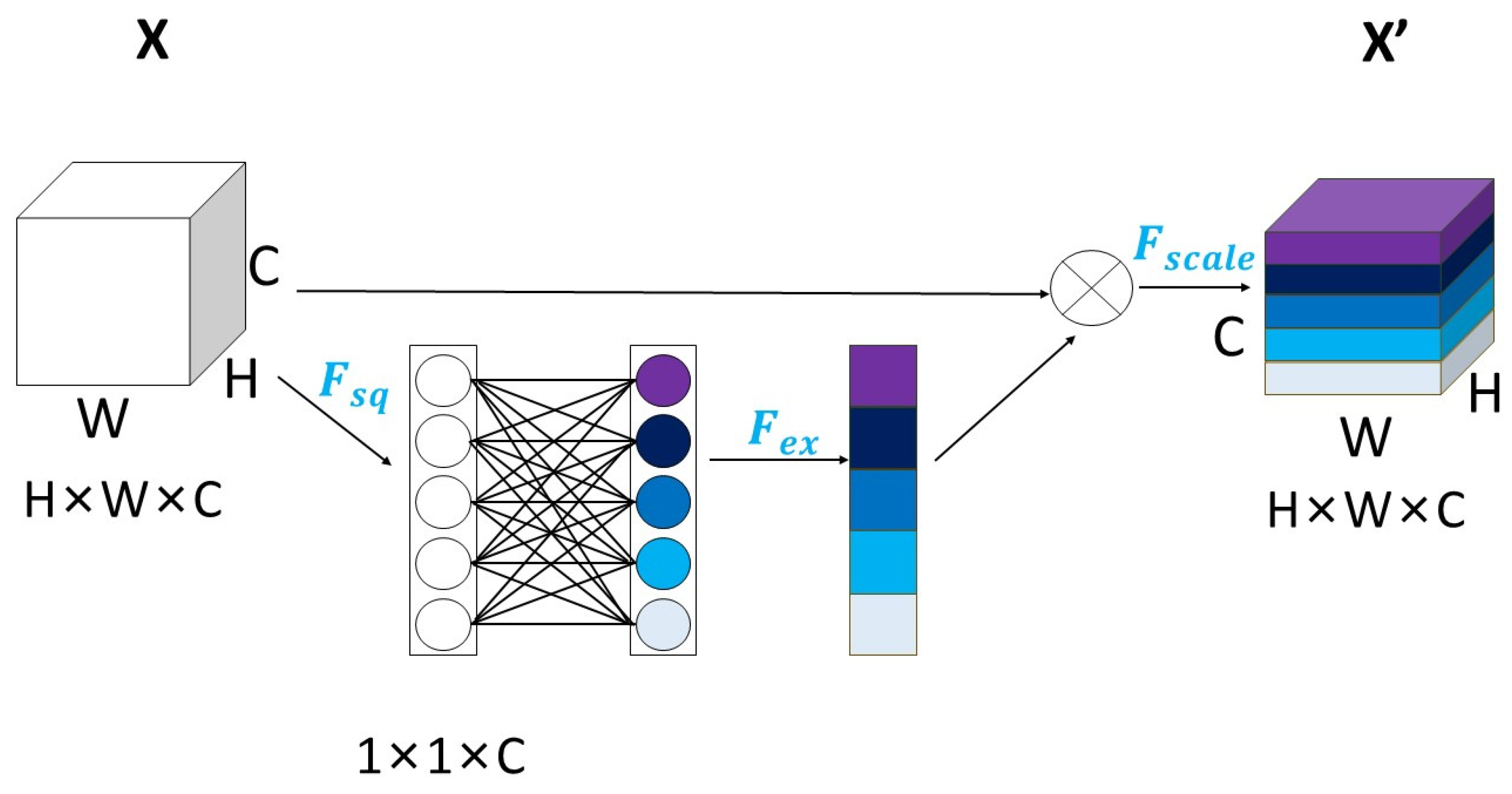
As a kind of channel attention mechanism, squeeze-and-excitation networks [31] (SE-Net) were considered first. SE-Net was the winner of classification at the final ImageNet contest in 2017. As a classic model of attention mechanism, the operation of SE-Net could be composed of three parts: squeeze, excitation and reweight. The schematic diagram is shown in Figure 3:
In Figure 3, different colors represent different features extracted from each channel. H and W denote the dimensions of the image pixels, while C represents the number of channels. F s q represents squeeze compression, which compresses three-dimensional feature data with the dimensions H × W × C into 1 × 1 × C data for ease of subsequent assignment. The calculation formula is as follows:
F s q ( u c ) = 1 H × W 1   i     H 1   j     W u c ( i , j )
F e x signifies excitation. The weights of the 1 × 1 × C data are assigned based on the importance of each channel, with higher weight given to more important channels at their corresponding locations. The calculation formula is:
F e x ( z , W ) = σ ( g ( z , W ) ) = σ ( W 2 δ ( W 1 z ) )
W 1 and W 2 are used to represent the two fully connected layers within the SE module. F s c a l e denotes reweighting, which is also known as scaling operation. It restores the data of 1 × 1 × C with weight acquisition into H × W × C, where each channel has been weighted to enhance deep learning network training effectiveness.
However, in practical applications of SE-Net, it has been observed that some significant information would be lost during the process of squeeze and capturing dependencies between all channels could be inefficient and unnecessary. To address this issue, ECA-Net is proposed. ECA-Net [32] is a lightweight attention-mechanism module that is developed from SE-Net. It was released at CVPR in 2020. It is characterized by easy plug and apply. Unlike traditional methods that assign weights to each channel based on their importance, ECA-Net utilizes a fully connected layer to achieve local cross-channel interaction within a fixed range. This method reduces computation and enhances the portability and efficiency of the structure. The schematic diagram of ECA-Net is shown in Figure 4:
In Figure 4, different colors represent different features extracted from each channel. GAP represents global average pooling; it compresses H × W × C data into 1 × 1 × C without dimensionality reduction and the features of each channel are aggregated. k has the function of connecting C channels, whose size is determined by the adaptive method. The computational formula is:
k = ψ ( C ) = | log 2 ( C ) γ + b γ | o d d
In this formula, b represents the offset of the linear mapping between k and the number of channels C , σ denotes feature redistribution for nonaggregated channels by assigning weights. It also signifies the relationship between obtained effects that undergo channel interaction and distributed weights. The formula is as follows:
ω = σ ( C 1 D k ( y ) )
C 1 D k represents the one-dimensional convolution of size k . In general, after using GAP aggregation convolution features, the ECA module first adaptively determines the kernel size k , then performs one-dimensional convolution and then applies a sigmoid function to learn local adjacent channel attention. This method was not only able to ensure the range of channel interaction and solve the dimensionality reduction problem but also improved performance and speed by reducing the computation and parameter quantity.

2.4. ECA-CRNN’s Entire Structure

2.4.1. CNN’s Structure

CNN is a feedforward neural network with a convolutional structure. As a classic deep learning model, CNN is widely applied in target recognition, image segmentation [33], face recognition and other fields. The CNN structure in this paper was improved from the literature [6]. It contained convolutional layer 1 with 128 filters and a 3 × 3 convolution kernel; convolutional layer 2 with 256 filters and a 3 × 3 convolution kernel; convolutional layer 3 with 256 filters and a 3 × 3 convolution kernel; and convolutional layer 4 with 128 filters and a 1 × 1 convolution kernel. The first three convolutional layers were utilized enough to extract features, the last one was utilized to fuse feature maps of other convolutional layers.
As the convolutional layer increased in depth and number, there was a higher likelihood of experiencing learning loss. Meanwhile, after extensive modifications and debugging of the ECA-CRNN model, we found that reducing the number of layers resulted in inadequate extraction of all relevant features, leading to a decline in classification accuracy. Conversely, increasing the number of layers not only increased the model size and prolonged training time but also exacerbated the vanishing gradient problem. To enhance training efficiency and reduce computational costs, we determined that utilizing four convolutional layers was optimal for accurately classifying emotions in our method.
As the pooling layers lead to a reduction in data size and our dataset is already limited, we chose to incorporate only one maxpool layer following the four convolutional layers to avoid the loss of crucial information. The maxpool layer was the size of 2 × 2. After the maxpool layer, a flattened layer and a flattenedfully connected layer were sequentially applied. The fully connected layer is also known as the dense layer in keras.
The ReLU activation function was utilized in the convolutional layer for linear correction [34]. The formula of ReLU is:
R e L U ( x ) { x , x > 0 0 , x 0
The four convolutional layers all had a stride of 1 and each one included an activation function as well as a batch normalization (BN) layer [35]. The calculation formulas of BN layer are:
μ = 1 m i = 1 m x i
σ = 1 m i = 1 m ( x i μ ) 2
x i ^ = x i μ σ 2 + ε
y i = γ x i ^ + β
B N ( x ) = ω x + b μ σ 2 + ε + β = γ ω σ 2 + ε x + γ σ 2 + ε ( b μ ) + β
Among these formulas, μ and σ represent the mean value and variance of each feature map, x i ^ represents the normalized data, y i could be seen as the output which is obtained through translation and scaling utilizing β and γ . β and γ act as shift factor and scale factor, respectively, and they are both learnable parameters, which means they cannot be fixed but could vary with each training batch. Upon completion of the training process, the total number of β and γ is the overall dataset size divided by batch size. By utilizing these parameters, the BN layer could inhibit internal covariate shift, so that the overall parameter remained relatively stable in a limited range. The BN layer could also recalibrate its other parameters to ensure controllability while enhancing network stability for optimal training outcomes.
The ECA-Net module was inserted after each convolutional layer, respectively, to ensure that the corresponding relationship between frequency bands could be better represented. The number of ECA-Net module followed that of convolutions. Because ECA-Net is a channel attention mechanism that generates channel weights, only after convolutions did spatial size become fixed, which did not affect the weights between channels, allowing for more comprehensive feature extraction. The structure of the convolutional neural network presented in this paper is shown in Figure 5:
Alpha dropout was utilized as a dropout layer following the fully connected layer to mitigate overfitting during training and maintain self-normalization. During the training process, alpha dropout set some elements to zero with the certain probability p drawn from the Bernoulli distribution. However, during each forward call, the remaining elements were scaled and shifted randomly to preserve the unit standard deviation. In this way, alpha dropout could ensure that mean and variance remained constant while negative saturation values were randomly activated to self-regularize the data [36]. To ensure a unit standard deviation output, alpha dropout was always paired with the SeLU activation function. The formula of SeLU is:
a = { λ α ( e x 1 ) , x < 0 λ x , x 0
For λ and α in the formula, their values are predetermined. SeLU ensures faster internal normalization compared to external normalization, resulting in quicker network convergence.

2.4.2. GRU’s Structure

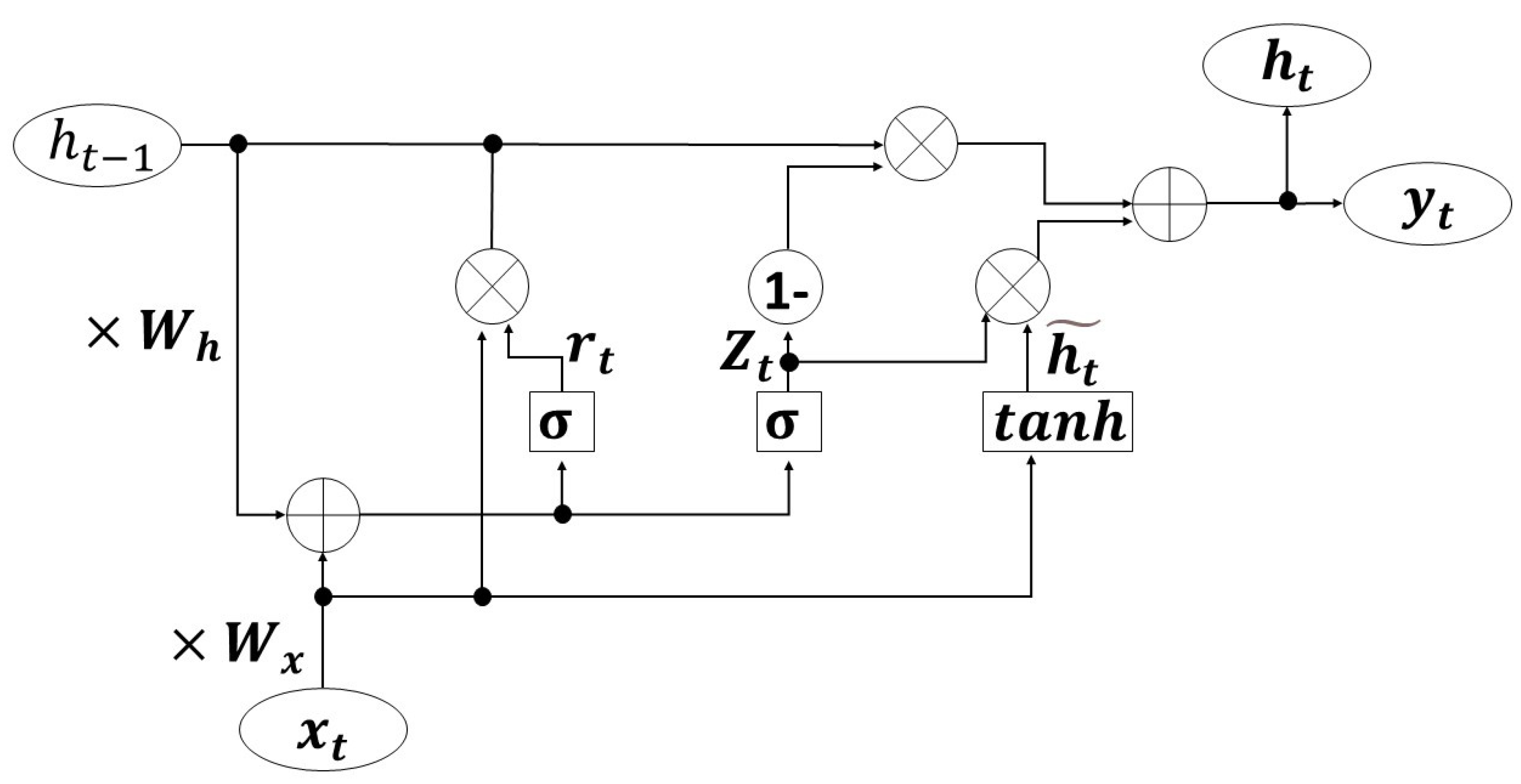
After applying CNN, the time sequence forecasting method should be considered for extracting temporal information. RNN possesses both internal feedback connections and feedforward connections between processing units, as well as the ability to memorize like a human. However, its susceptibility to short-term memory may compromise its performance. When dealing with long sequences, it becomes challenging for information to propagate from earlier time steps to later ones, leading to issues with gradient vanishing or exploding. GRU is an improvement of RNN that could effectively address this issue, while also resolving the problem of long-term dependencies [37]. The basic diagram of GRU is shown in Figure 6:
In Figure 6, tanh represents the activation function, which could regulate the flow of values within the network and constrain them between −1 and 1. The formula of tanh is:
t a n h ( x ) = e x e x e x + e x
σ represents the sigmoid function. It ranges from 0 to 1, so it could serve as a gating signal for implementing memory and forgetting operations. The formula of σ is:
s i g m o i d ( x ) = 1 1 + e x
The circular part represents the operation and the square part represents the layer structure. Figure 6 indicates that the GRU network comprises a tanh layer and two sigmoid layers.
The equations utilized for computation are as follows:
z t = σ ( W z h h t 1 + W z x x t )
r t = σ ( W r h h t 1 + W r x x t )
h t ˜ = tanh ( W r h ( r t h t 1 ) + W x x t )
h t = ( 1 z t ) h t 1 + z t h t ˜
Among these formulas, x t represents the input in the current state, h t 1 represents the retained information from the previous state and W x and W h are the weight matrices calculated for x t and h t 1 , respectively. r t represents the reset gate, which combines the current state with the past memory. z t represents the update gate, which is used to determine how much previous state information is retained in the current state and how much information is required at the next moment. Therefore, ( 1 z t ) represents the degree of information decay. The closer z t approaches 1, the more information is retained. Conversely, the closer z t approaches 0, the more information is forgotten. h t ˜ represents a hidden state that may or may not be selected based on its relevance to the current context. h t is the final state that integrates previous memory and current input to generate output for subsequent GRU units.
At the end of GRU, a softmax classifier is utilized as a generalization of a logistic regression that extends binary classification to multiple classes [38]. The formula of softmax is:
f j ( z ) = e z j k e z k
The principle of the softmax classifier is to constrain the classification outputs within a range of 0 to 1, ensuring that all values could be summed up to 1. In order to convert the scores into probabilities, it is necessary to apply the sigmoid function and utilize the cross-entropy loss function. The formula of cross entropy loss is:
L C E = i = 1 n t i log ( p i )
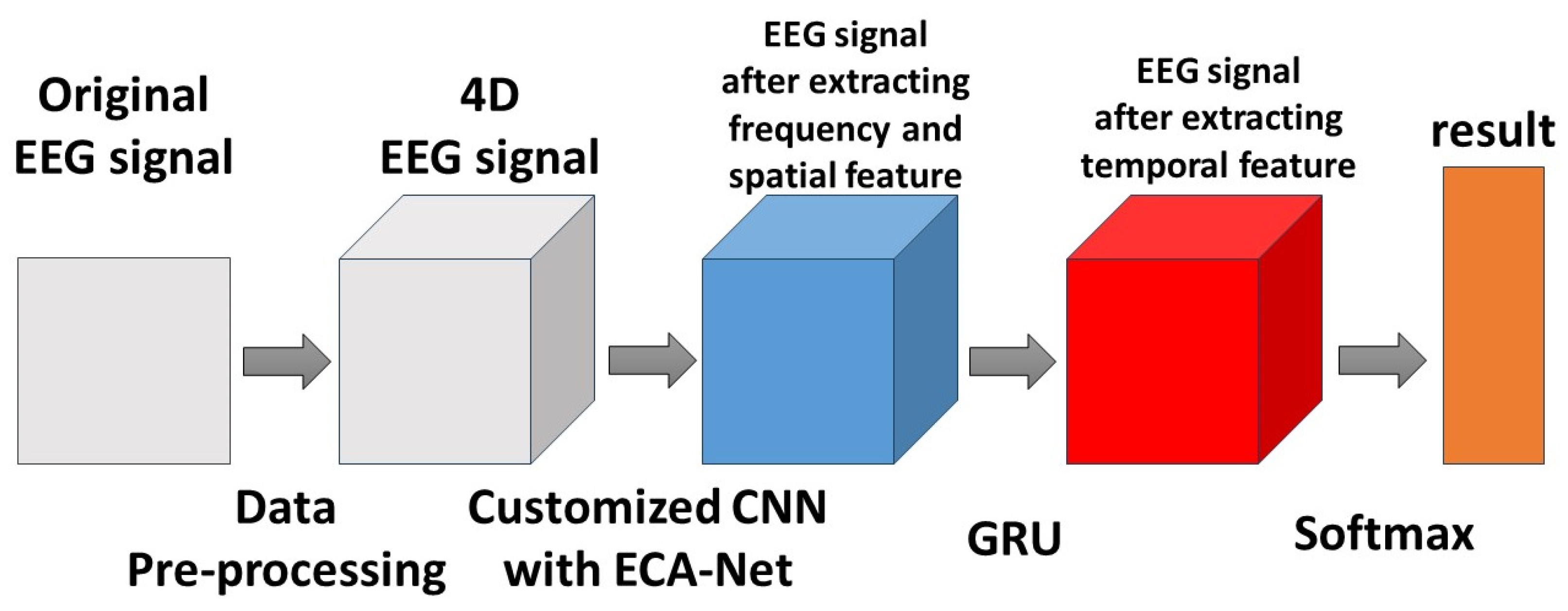
In the formula, t i is the real value and p i is the output obtained from the softmax function. The final result of cross entropy loss evaluates the performance of the classification model. The complete model of ECA-CRNN is shown in Figure 7.
The diagram of feature extraction using ECA-CRNN is shown in Figure 8.

3. Experiment

3.1. Experimental Environment and Parameter Setting

The hardware utilized in this paper employs a computer equipped with a 13th Gen Intel(R) Core(TM) i7-13700HX CPU, 16.00 GB of RAM and NVIDIA GeForce RTX 4060 graphics card with 8G memory. The software environment is the Windows11 operating system, which runs on the python3.9 programming environment and utilizes the tensorflow framework while invoking library functions such as keras, numpy, math and matplotlib among others. The entire program is executed using GPU acceleration.
In our experiment, since the DEAP dataset comprises four evaluation indexes, only valence and arousal had the most significant impact on emotion recognition. Therefore, these two indices were the focus of verification. The batch size for data input into the network was set at 64. We used the Adam optimization for the entire network with a learning rate of 0.001. To prevent overfitting during the training process, the value of dropout in the alpha dropout layer was set at 0.1 and the units of GRU were set at 128. In addition, in the ECA-Net module, the values of γ and b were adjusted to 2 and 1, respectively, in order to maintain a balance between the number of frequency bands and the size of the convolution kernel.
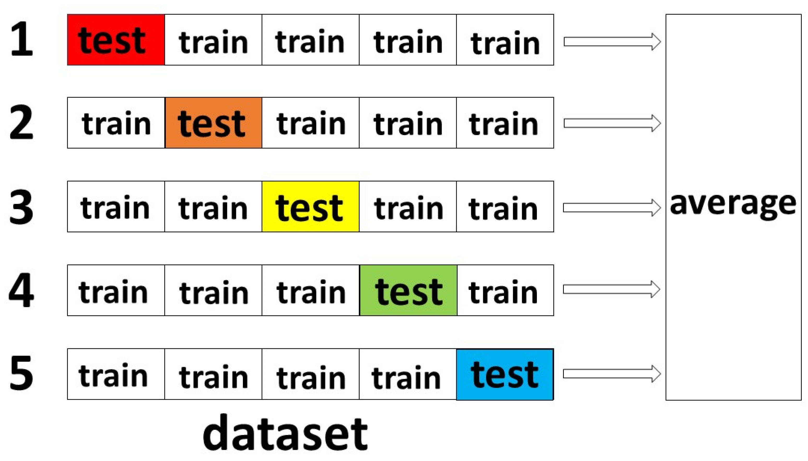
To enhance the efficacy of training, testing and statistical process, a five-fold cross-validation method was employed in the training process. Each subject’s EEG data were trained and tested as an individual experiment to avoid any mixing of their data. Therefore, each experiment could be evaluated independently with a total of 32 experiments. The diagram of five-fold cross-validation is shown in Figure 9:
In Figure 9, the colored parts represent the different test sets, and the white parts represent the training sets. The dataset comprising of 32 subjects is partitioned into five equally different parts and each part was treated as a test set in turn while the remaining four parts served as training sets. The final result was obtained by averaging the results from all five tests.

3.2. Data Preprocessing

In order to extract the different features easily and accurately, it was necessary to preprocess the original DEAP dataset first. Considering that the DEAP dataset had been sampled in advance, band pass filtering within a range of 4–50 Hz could be applied to eliminate delta waves as well as the industrial frequency spurious noise. The initial step involved segmenting the signal into fixed temporal segments of a specific size, t. Subsequently, the data were partitioned into four frequency bands using a Butterworth filter. Then the differential DE features were extracted from each frequency band with a sampling time of 0.5 s [39,40], which yielded relatively superior results. Finally, the spatial information was integrated with the aforementioned features to generate the 4D feature. This operation ensured that the preprocessing data were resized from (40, 40, 8064) to (4800, 4, 8, 9). Among it, 4800 represents 40 one-minute videos with a sampling time of 0.5 s, four represents four frequency bands and (8, 9) represents the spatial information.

3.3. Experimental Processing and Data Comparison

In terms of the training process, Table 1 presents a comprehensive overview of the specific details pertaining to our CNN model.
When the preprocessed data were fed into the network, it was found that varying segment lengths in the experiment yielded different results. Table 2 shows how the recognition accuracy varies with the length of segment when the epoch is set to 100 for a while:
From the data, it is evident that optimal results were achieved when the time duration was set to 4 s, with recognition accuracy and standard deviation significantly surpassing other durations. The accuracy of valence and arousal reached 95.45% and 95.12% and the standard deviation reached 1.28% and 1.55%. Considering that the data fragment of 60 s could only be divisible by time intervals of 10 s and 12 s, as well as all integers less than or equal to six, and larger time periods such as 10 and 12 s would lose their significance in segmentation and fail to achieve the purpose of refining the data, the method took four as the ultimate value of t.
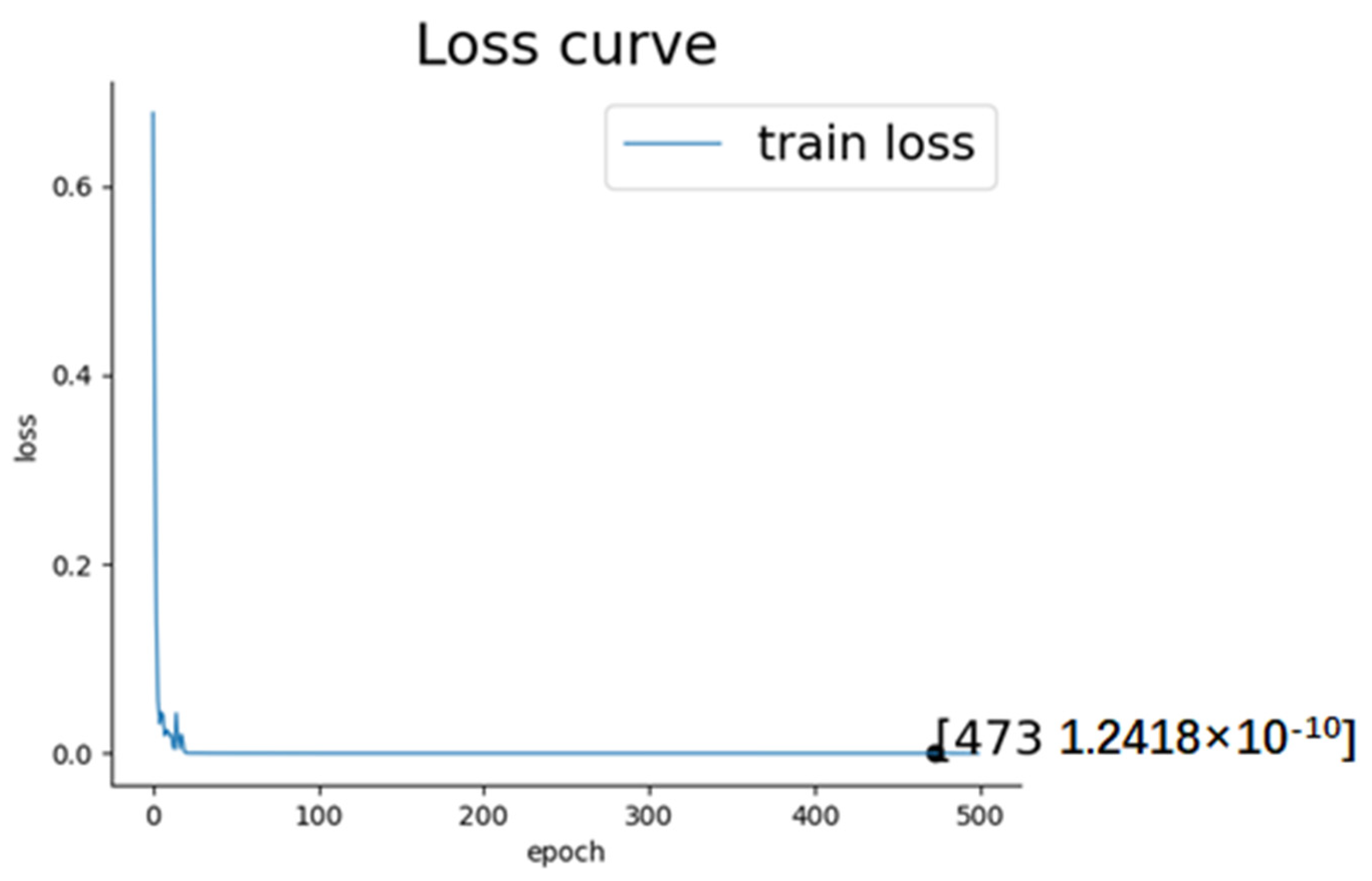
It was also found that the epoch exerted an influence on the experimental outcome. Because our experiment involved a five-fold cross-validation process and the subjects’ data were divided into 32 independent parts for training and testing, have decided to evaluate performance based on the average loss across these 32 datasets. The figure of average loss curve during training process is shown in Figure 10:
The loss curve shows that the average loss reached its minimum and remained stable when the training epoch approached 473. Table 3 also shows the results of how the recognition accuracy for arousal and valence changed with epoch while keeping other experiment conditions constant:
It can be seen that when the epoch reached 473, the accuracy of valence and arousal reached 95.70% and 95.33% with a standard deviation of 1.16% and 1.45%. In contrast, inadequate feature extraction resulted in lower accuracy when it did not reach this threshold value. However, exceeding an epoch count of 473 led to overfitting issues that caused a slight decline in model accuracy.
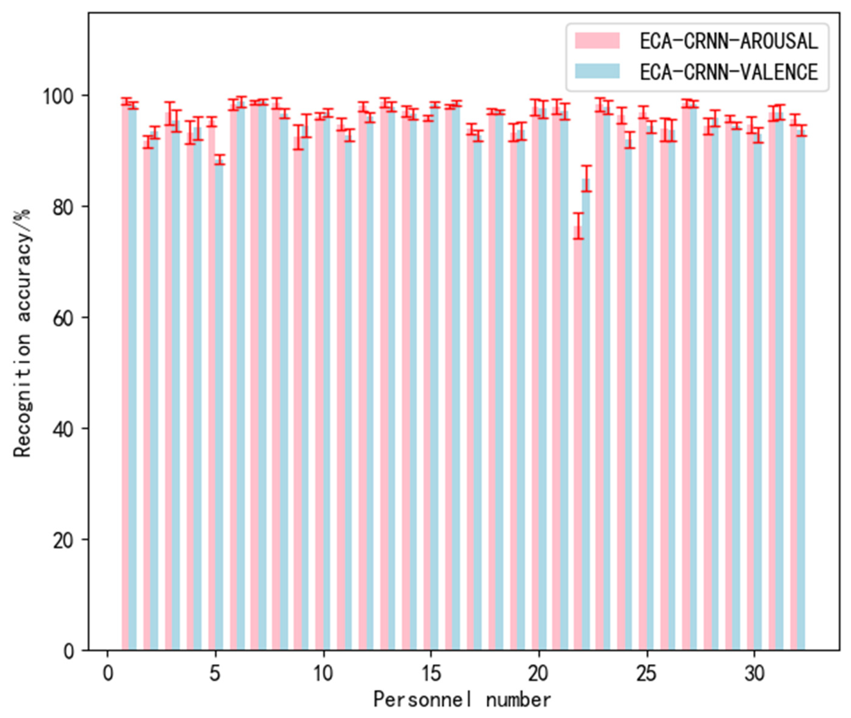
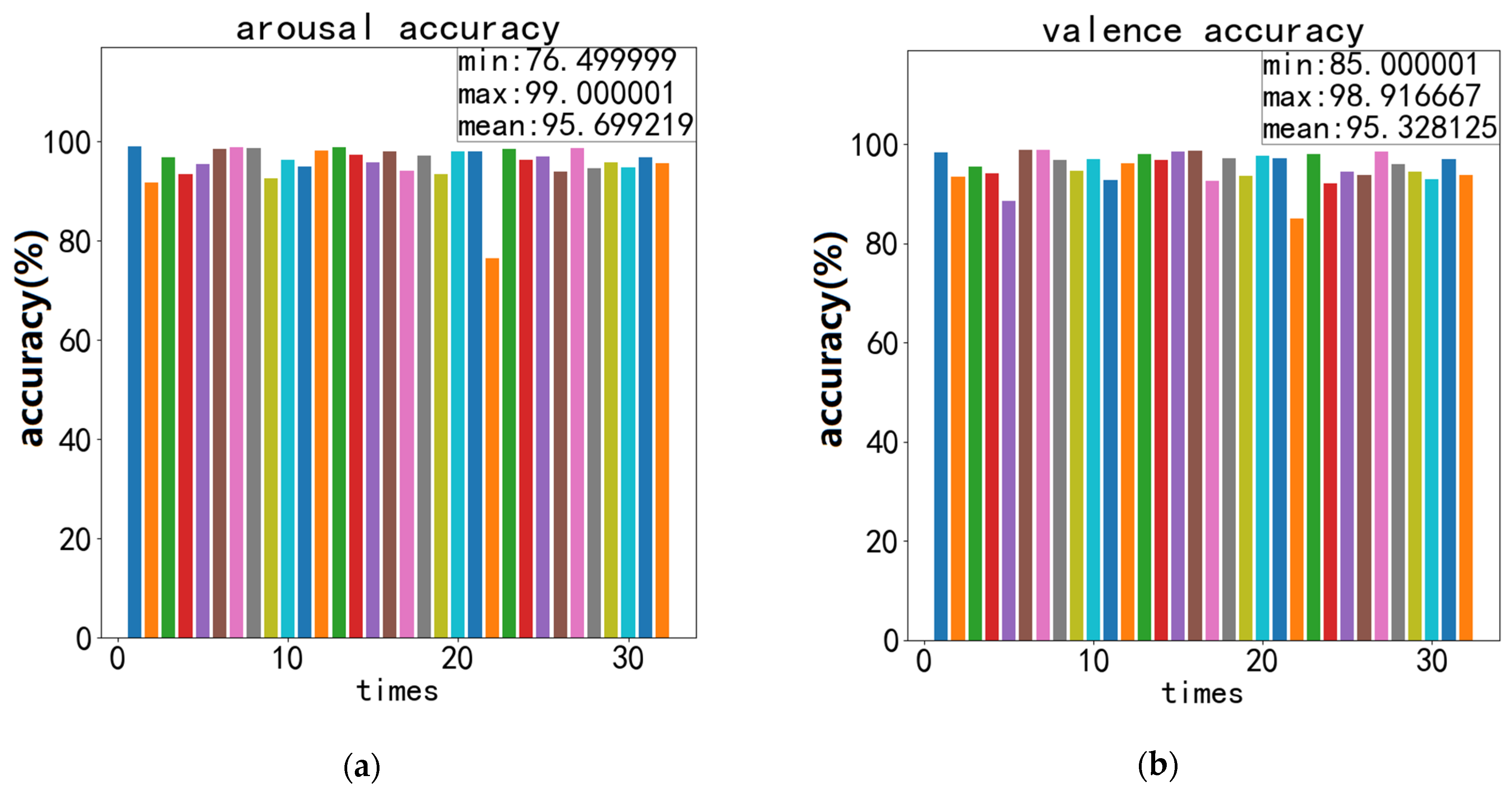
The recognition accuracy and standard deviation of valence and arousal obtained during the experiment are shown in Figure 11, Figure 12 and Figure 13:
We verified several methods utilizing the structure and parameters presented in the original papers tested on the DEAP datasets with five-fold cross-validation, resulting in some experimental data. The theoretical results claimed in the original paper are stated in introduction. In addition, our tests demonstrate that these theoretical outcomes are comparable to actual experimental results, with recognition accuracy and standard deviation closely resembling those reported in literature. Table 4 shows our experimental data:

4. Discussion

In terms of the results, the ECA-CRNN outperformed most existing methods for emotion recognition. By comparison with the literature [5], it is obvious that the EEG signals after processing were more complete and more comprehensive than the original data set. The literature [6] confirmed that the utilization of multidimensional information can enhance the accuracy of classification results and a single CNN cannot extract all the features because it only concerns spatial and frequency information in EEG signals. Refs. [8,10] both confirmed that the combination of CNN and LSTM has a high accuracy in emotion recognition, but the training speed of the LSTM is slower in time sequence forecast methods. Although PCRNN [9] also utilizes the combination of CNN and LSTM, it turns out that our ECA-CRNN had a better performance. The reason why is that sequential structure can extract more complete features than parallel structure when using CNN and LSTM.
Compared to the 4D-CRNN model [12], our method distinguished itself by incorporating four ECA-Net modules, which enabled us to highlight the most effective channels, take into account the impact of adjacent frequency bands during feature extraction and strengthen the relationship between frequency bands. Additionally, ECA-Net is a local cross-channel interaction strategy without dimensionality reduction, which can be effectively implemented through one-dimensional convolution, so it involves only a few parameters and has little effect on the training speed. Moreover, proper cross-channel interactions could also significantly reduce complexity while maintaining performance, resulting in more complete and diverse features being extracted and better recognition performance. In addition, we incorporated batch normalization and alpha dropout layers in comparison to 4D-CRNN. The BN layer could effectively suppress internal covariate shift and ensure that each layer of data was transformed into a fixed state, thereby maintaining the overall parameters within a limited range. This approach accelerates training speed and convergence, controls gradient explosion and prevents vanishing gradients as well as overfitting. In general, the BN layer improved the stability of CNN in the process of feature extraction to make features more accurate. The alpha dropout layer can maintain the input’s mean and standard deviation while keeping the data self-normalized, thereby preventing overfitting caused by excessive epochs. We also implemented structural improvements to the CNN, such as reducing the size of the convolution kernel in order to decrease both parameters and computation and accelerate the process of feature extraction. These are the main reasons why the proposed method is superior to the 4D-CRNN method.
In addition, our results demonstrate a significant improvement in emotion recognition accuracy across all subjects for the DEAP dataset compared to 4D-CRNN. However, subject no. 22 still exhibited low accuracy and only showed marginal improvement. On the one hand, this could be attributed to subject no. 22’s lack of subjective evaluation during the experiment, minimal mood fluctuations due to individual differences or measurement errors caused by the experimental equipment. On the other hand, the attention module of the efficient channel mechanism extracted features based on nearby channel influence during weight allocation. As a result, the inaccurate data’s learning effect deteriorates when influenced by other channels.
But there are still some problems and limitations of the ECA-CRNN model. For example, the structure of CNN could be further optimized. Although the number of layers has been adjusted to the optimum, some parameters could be adjusted to change with the training process. This adjustment makes the model more compatible with the data but might come with uncertain errors. Also, if our method adopts the structure that each parallel branch extracts one single feature, this might improve the recognition accuracy. But it also leads to lower efficiency and slower training speed, which results in the need to reconsider calculation costs. The aspect of data processing can also be optimized. If we take the sparse map as the spatial information, the relationship of space and frequency might be emphasized further. But it unquestionably will increase computing costs and lead to a slower training process.
Overall, the characteristics compared to other models are shown in the Table 5:

5. Conclusions

This paper proposes a new method based on deep learning and attention mechanism for identifying individual emotions according to EEG signals, which raises some new ideas. We propose a novel model named ECA-CRNN, which integrates customized CNN and GRU while inserting the Efficient Channel Attention Module for the first time in emotion recognition using EEG signals. During the phase of data processing, we turned the original EEG signal into four-dimensional data as input. During the stage of feature extraction, our customized CNN extracts spatial and DE frequency features while GRU focuses on extracting frequency features. The ECA-CRNN model enhanced the accuracy of valence and arousal identification on the DEAP dataset, achieving 95.70% and 95.33%, respectively, and the standard deviations for valence and arousal identification were 1.16% and 1.45%, which are superior to most existing methods. Our experimental results show that the lower standard deviation of ECA-CRNN presents its ability to mitigate the impact of random errors, minimize false recognition rates and prevent accidents in limited experimental conditions or with a small number of experiments. Our results also ensure that every identification achieves maximum accuracy. In terms of results, the recognition accuracy we achieved may not represent the optimal data compared to some latest methods due to the experimental conditions, measurement deviation during DEAP dataset collection, random variables, unknow errors, etc. Nonetheless, with regard to the ultimate outcome, our attempt to utilize ECA-Net in CNN for emotional recognition is both feasible and significant, thereby demonstrating its practical applicability in emotion recognition. Additionally, we have also confirmed the enhancing effect of ECA-Net on lightweight networks.

Author Contributions

Conceptualization, Y.S.; methodology, Y.S. and Y.Y.; software, Y.S. and Y.Y.; validation, Y.S., Y.Y. and P.X.; formal analysis, P.X.; investigation, Y.Y.; resources, Y.S. and P.X.; data curation, Y.S. and Y.Y.; writing—original draft preparation, Y.Y.; writing—review and editing, Y.S. and P.X.; visualization, P.X. and Y.Y.; supervision, Y.S. and P.X. All authors have read and agreed to the published version of the manuscript.

Funding

This research was funded by the Natural Science Foundation of Liaoning province, grant number: 2022-KF-12-11.

Data Availability Statement

DEAP dataset source: http://www.eecs.qmul.ac.uk/mmv/datasets/deap/ (accessed on 20 October 2021).

Conflicts of Interest

The authors declare no conflict of interest.

References

  1. Lux, V.; van Ommen, C. The generational brain: Introduction. Theory Psychol. 2016, 26, 561–571. [Google Scholar] [CrossRef]
  2. Saarimaki, H.; Ejtehadian, L.F.; Glerean, E.; Jaaskelainen, I.P.; Vuilleumier, P.; Sams, M.; Nummenmaa, L. Distributed affective space represents multiple emotion categories across the human brain. Soc. Cogn. Affect. Neurosci. 2018, 13, 471–482. [Google Scholar] [CrossRef] [PubMed]
  3. Zhang, Y.; Cui, C.; Zhong, S.H. EEG-Based Emotion Recognition via Knowledge-Integrated Interpretable Method. Mathematics 2023, 11, 1424. [Google Scholar] [CrossRef]
  4. Chen, J.X.; Zhang, P.W.; Mao, Z.J.; Huang, Y.F.; Jiang, D.M.; Zhang, A.N. Accurate EEG-Based Emotion Recognition on Combined Features Using Deep Convolutional Neural Networks. IEEE Access 2019, 7, 44317–44328. [Google Scholar] [CrossRef]
  5. Wang, Y.; Huang, Z.; Mccane, B.; Neo, P. EmotioNet: A 3-D Convolutional Neural Network for EEG-based Emotion Recognition. In Proceedings of the 2018 International Joint Conference on Neural Networks (IJCNN), Rio de Janeiro, Brazil, 8–13 July 2018; pp. 1–7. [Google Scholar]
  6. Yang, Y.; Wu, Q.; Fu, Y.; Chen, X. Continuous Convolutional Neural Network with 3D Input for EEG-Based Emotion Recognition. Neural. Inf. Process. 2018, 11307, 433–443. [Google Scholar]
  7. Li, J.P.; Zhang, Z.X.; He, H.G. Hierarchical Convolutional Neural Networks for EEG-Based Emotion Recognition. Cogn. Comput. 2018, 10, 368–380. [Google Scholar] [CrossRef]
  8. Zhang, Y.Q.; Chen, J.L.; Tan, J.H.; Chen, Y.X.; Chen, Y.Y.; Li, D.H.; Yang, L.; Su, J.; Huang, X.; Che, W.L. An Investigation of Deep Learning Models for EEG-Based Emotion Recognition. Front. Neurosci. 2020, 14, 622759. [Google Scholar] [CrossRef]
  9. Yang, Y.; Wu, Q.; Qiu, M.; Wang, Y.; Chen, X. Emotion Recognition from Multi-Channel EEG through Parallel Convolutional Recurrent Neural Network. In Proceedings of the 2018 International Joint Conference on Neural Networks (IJCNN), Rio de Janeiro, Brazil, 8–13 July 2018; pp. 1–7. [Google Scholar]
  10. Iyer, A.; Das, S.S.; Teotia, R.; Maheshwari, S.; Sharma, R.R. CNN and LSTM based ensemble learning for human emotion recognition using EEG recordings. Multimed. Tools Appl. 2023, 82, 4883–4896. [Google Scholar] [CrossRef]
  11. Wilaiprasitporn, T.; Ditthapron, A.; Matchaparn, K.; Tongbuasirilai, T.; Banluesombatkul, N.; Chuangsuwanich, E. Affective EEG-Based Person Identification Using the Deep Learning Approach. IEEE Trans. Cogn. Dev. Syst. 2020, 12, 486–496. [Google Scholar] [CrossRef] [Green Version]
  12. Shen, F.Y.; Dai, G.J.; Lin, G.; Zhang, J.H.; Kong, W.Z.; Zeng, H. EEG-based emotion recognition using 4D convolutional recurrent neural network. Cogn. Neurodyn. 2020, 14, 815–828. [Google Scholar] [CrossRef]
  13. Kim, G.I.; Jang, B. Petroleum Price Prediction with CNN-LSTM and CNN-GRU Using Skip-Connection. Mathematics 2023, 11, 547. [Google Scholar] [CrossRef]
  14. Koelstra, S.; Muhl, C.; Soleymani, M.; Lee, J.S.; Yazdani, A.; Ebrahimi, T.; Pun, T.; Nijholt, A.; Patras, I. DEAP: A Database for Emotion Analysis Using Physiological Signals. IEEE Trans. Affect. Comput. 2012, 3, 18–31. [Google Scholar] [CrossRef] [Green Version]
  15. Khateeb, M.; Anwar, S.M.; Alnowami, M. Multi-Domain Feature Fusion for Emotion Classification Using DEAP Dataset. IEEE Access 2021, 9, 12134–12142. [Google Scholar] [CrossRef]
  16. Joshi, V.M.; Ghongade, R.B.; Joshi, A.M.; Kulkarni, R.V. Deep BiLSTM neural network model for emotion detection using cross-dataset approach. Biomed. Signal Process. Control 2022, 73, 103407. [Google Scholar] [CrossRef]
  17. Menezes, M.L.R.; Samara, A.; Galway, L.; Sant’Anna, A.; Verikas, A.; Alonso-Fernandez, F.; Wang, H.; Bond, R. Towards emotion recognition for virtual environments: An evaluation of eeg features on benchmark dataset. Pers. Ubiquitous Comput. 2017, 21, 1003–1013. [Google Scholar] [CrossRef] [Green Version]
  18. Choi, E.; Kim, D. Arousal, Valence and Liking Classification Model Based on Deep Belief Network and DEAP Dataset for Mental Healthcare Management. Basic Clin. Pharmacol. Toxicol. 2019, 124, 214–215. [Google Scholar]
  19. Singh, U.; Shaw, R.; Patra, B.K. A data augmentation and channel selection technique for grading human emotions on DEAP dataset. Biomed. Signal Process. Control 2023, 79, 104060. [Google Scholar] [CrossRef]
  20. Lu, H.M.; Wan, M.; Sangaiah, A.K. Human Emotion Recognition Using an EEG Cloud Computing Platform. Mob. Netw. Appl. 2020, 25, 1023–1032. [Google Scholar] [CrossRef]
  21. Huang, D.M.; Chen, S.T.; Liu, C.; Zheng, L.; Tian, Z.H.; Jiang, D.Z. Differences first in asymmetric brain: A bi-hemisphere discrepancy convolutional neural network for EEG emotion recognition. Neurocomputing 2021, 448, 140–151. [Google Scholar] [CrossRef]
  22. De Witte, S.; Klooster, D.; Dedoncker, J.; Duprat, R.; Remue, J.; Baeken, C. Left prefrontal neuronavigated electrode localization in tDCS: 10-20 EEG system versus MRI-guided neuronavigation. Psychiatry Res. Neuroimaging 2018, 274, 1–6. [Google Scholar] [CrossRef]
  23. Xu, G.X.; Guo, W.H.; Wang, Y.J. Subject-independent EEG emotion recognition with hybrid spatio-temporal GRU-Conv architecture. Med. Biol. Eng. Comput. 2023, 61, 61–73. [Google Scholar] [CrossRef]
  24. Demir, F.; Sobahi, N.; Siuly, S.; Sengur, A. Exploring Deep Learning Features for Automatic Classification of Human Emotion Using EEG Rhythms. IEEE Sens. J. 2021, 21, 14923–14930. [Google Scholar] [CrossRef]
  25. Cui, D.; Xuan, H.Y.; Liu, J.; Gu, G.H.; Li, X.L. Emotion Recognition on EEG Signal Using ResNeXt Attention 2D-3D Convolution Neural Networks. Neural Process. Lett. 2022, 1–5. [Google Scholar] [CrossRef]
  26. Yin, Y.Q.; Zheng, X.W.; Hu, B.; Zhang, Y.; Cui, X.C. EEG emotion recognition using fusion model of graph convolutional neural networks and LSTM. Appl. Soft Comput. 2021, 100, 106954. [Google Scholar] [CrossRef]
  27. Zheng, W.L.; Lu, B.L. Investigating Critical Frequency Bands and Channels for EEG-Based Emotion Recognition with Deep Neural Networks. IEEE Trans. Auton. Ment. Dev. 2015, 7, 162–175. [Google Scholar] [CrossRef]
  28. Mehmood, R.M.; Du, R.Y.; Lee, H.J. Optimal Feature Selection and Deep Learning Ensembles Method for Emotion Recognition From Human Brain EEG Sensors. IEEE Access 2017, 5, 14797–14806. [Google Scholar] [CrossRef]
  29. Hwang, S.; Hong, K.; Son, G.; Byun, H. Learning CNN features from DE features for EEG-based emotion recognition. Pattern Anal. Appl. 2020, 23, 1323–1335. [Google Scholar] [CrossRef]
  30. Zheng, W.L.; Zhu, J.Y.; Lu, B.L. Identifying Stable Patterns over Time for Emotion Recognition from EEG. IEEE Trans. Affect. Comput. 2019, 10, 417–429. [Google Scholar] [CrossRef] [Green Version]
  31. Hu, J.; Shen, L.; Albanie, S.; Sun, G.; Wu, E.H. Squeeze-and-Excitation Networks. IEEE Trans. Pattern Anal. Mach. Intell. 2020, 42, 2011–2023. [Google Scholar] [CrossRef] [Green Version]
  32. Wang, Q.L.; Wu, B.G.; Zhu, P.F.; Li, P.H.; Zuo, W.M.; Hu, Q.H. ECA-Net: Efficient channel attention for deep convolutional neural networks. arXiv 2020, arXiv:1910.03151. [Google Scholar]
  33. Zhao, Y.X.; Man, K.L.; Smith, J.; Siddique, K.; Guan, S.U. Improved two-stream model for human action recognition. Eurasip J. Image Video Process. 2020, 2020, 24. [Google Scholar] [CrossRef]
  34. Gonon, L.; Schwab, C. Deep ReLU neural networks overcome the curse of dimensionality for partial integrodifferential equations. Anal. Appl. 2023, 21, 1–47. [Google Scholar] [CrossRef]
  35. Yang, S.Y.; Hao, K.R.; Ding, Y.S.; Liu, J. Vehicle Driving Direction Control Based on Compressed Network. Int. J. Pattern Recognit. Artif. Intell. 2018, 32, 1850025. [Google Scholar] [CrossRef]
  36. Yang, W.W.; Jia, C.X.; Liu, R.F. Construction and Simulation of the Enterprise Financial Risk Diagnosis Model by Using Dropout and BN to Improve LSTM. Secur. Commun. Netw. 2022, 2022, 4767980. [Google Scholar] [CrossRef]
  37. Chen, J.X.; Jiang, D.M.; Zhang, N. A Hierarchical Bidirectional GRU Model With Attention for EEG-Based Emotion Classification. IEEE Access 2019, 7, 118530–118540. [Google Scholar] [CrossRef]
  38. Siuly, S.; Guo, Y.H.; Alcin, O.F.; Li, Y.; Wen, P.; Wang, H. Exploring deep residual network based features for automatic schizophrenia detection from EEG. Phys. Eng. Sci. Med. 2023, 46, 561–574. [Google Scholar] [CrossRef] [PubMed]
  39. Issa, S.; Peng, Q.; You, X. Emotion Classification Using EEG Brain Signals and the Broad Learning System. IEEE Trans. Syst. Man Cybern.-Syst. 2021, 51, 7382–7391. [Google Scholar] [CrossRef]
  40. Asghar, M.A.; Khan, M.J.; Rizwan, M.; Shorfuzzaman, M.; Mehmood, R.M. AI inspired EEG-based spatial feature selection method using multivariate empirical mode decomposition for emotion classification. Multimed. Syst. 2022, 28, 1275–1288. [Google Scholar] [CrossRef] [PubMed]
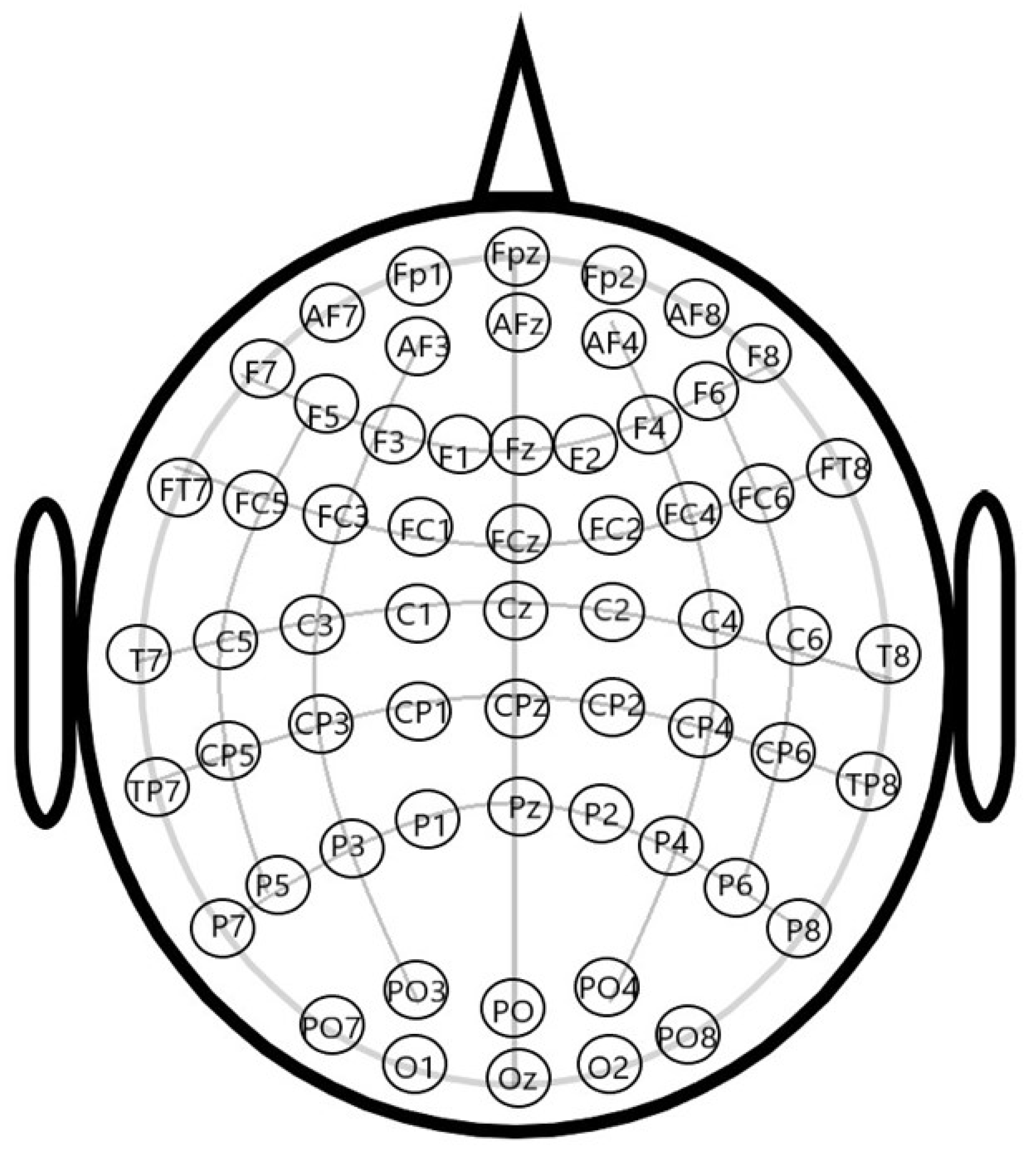
Figure 1. The diagram of 10–20 system.
Electronics 12 02900 g001
Figure 2. The diagram of data processing.
Electronics 12 02900 g002
Figure 3. The diagram of SE-Net.
Electronics 12 02900 g003
Figure 4. The diagram of ECA-Net.
Electronics 12 02900 g004
Figure 5. The structure of CNN in this paper.
Electronics 12 02900 g005
Figure 6. The diagram of GRU.
Electronics 12 02900 g006
Figure 7. The structure of ECA-CRNN.
Electronics 12 02900 g007
Figure 8. The diagram of extracting features.
Electronics 12 02900 g008
Figure 9. The diagram of five-fold cross-validation.
Electronics 12 02900 g009
Figure 10. ECA-CRNN’s valence and arousal accuracy for DEAP.
Electronics 12 02900 g010
Figure 11. Overall performance of ECA-CRNN model on DEAP.
Electronics 12 02900 g011
Figure 12. Recordings of ECA-CRNN’s best recognition accuracy on DEAP: (a) accuracy of arousal; (b) accuracy of valence.
Electronics 12 02900 g012
Figure 13. Recordings of ECA-CRNN’s best recognition standard deviation on DEAP: (a) standard deviation of arousal; (b) standard deviation of valence.
Electronics 12 02900 g013
Table 1. Our CNN’s layers and related parameters.
Layer (Type)Output ShapeActivationSize of Filter and PoolingNumber of Filters
conv1 (Conv2D)(None, 8, 9, 128)relu3 × 3128
batch_normalization (BatchNormalization)(None, 8, 9, 128)
eca1 (ECA)(None, 8, 9, 128)
conv2 (Conv2D)(None, 8, 9, 256)relu3 × 3256
batch_normalization (BatchNormalization)(None, 8, 9, 256)
eca2 (ECA)(None, 8, 9, 256)
conv3 (Conv2D)(None, 8, 9, 256)relu3 × 3256
batch_normalization (BatchNormalization)(None, 8, 9, 256)
eca3 (ECA)(None, 8, 9, 256)
Conv4 (Conv2D)(None, 8, 9, 128)relu1 × 1128
batch_normalization (BatchNormalization)(None, 8, 9, 128)
eca4 (ECA)(None, 8, 9, 128)
pool (MaxPooling2D)(None, 4, 4, 128) 2 × 2
fla1 (Flatten)(None, 2048)
dense1 (Dense)(None, 512)selu
alpha_dropout (AlphaDropout)(None, 512)
Table 2. Results with different value of t.
t (s)Arousal ((Acc ± Std)%)Valence ((Acc ± Std)%)
193.74 ± 2.0293.51 ± 2.14
293.98 ± 1.9393.65 ± 2.27
394.27 ± 1.5193.82 ± 1.92
495.45 ± 1.2895.12 ± 1.55
594.14 ± 1.8493.86 ± 2.18
694.07 ± 1.2993.75 ± 1.96
Table 3. Result with different epochs.
EpochsArousal ((Acc ± Std)%)Valence ((Acc ± Std)%)
10094.06 ± 2.0993.58 ± 2.24
20094.44 ± 1.8694.12 ± 1.76
30094.96 ± 1.5494.71 ± 1.83
40095.21 ± 1.9094.87 ± 1.61
47395.70 ± 1.1695.33 ± 1.45
50095.69 ± 1.2295.21 ± 1.87
60095.65 ± 2.1395.24 ± 1.88
Table 4. Results compared to other methods validated on DEAP.
MethodsArousal ((Acc ± Std)%)Valence ((Acc ± Std)%)
EmotioNet [5]73.24 ± 3.1372.16 ± 3.26
CCNN [6]90.15 ± 2.8789.41 ± 2.75
PCRNN [9]90.98 ± 3.2190.73 ± 2.94
Three-dimensional CNN [12]91.96 ± 2.8490.95 ± 2.52
4D-CRNN [12]94.52 ± 3.5994.18 ± 2.88
ECA-CRNN(ours)95.70 ± 1.1695.33 ± 1.45
Table 5. The comparison between ECA-CRNN and other methods.
ModelsCharacteristics
EmotioNet [5]Utilizing 3D convolution kernels to extract spatial-temporal information in the first half of the model and extracting temporal features in the second half but disregarding frequency information
CCNN [6]Building a customized continuous CNN model, but only focusing on frequency and spatial information
HCNN [7]Organizing differential entropy features across channels, but only attending to frequency and spatial information
PCRNN [9]By adopting a parallel branch structure, CNN and LSTM can extract distinct features from the raw EEG signals, but ignoring the interaction between space and time
Ensemble model [10]Refining a three-branch model to capture more information, albeit at the cost of increased parameters and complexity
4D-CRNN [12]Using DE features to construct four-dimensional features, focusing on frequency, spatial and temporal information, but ignoring the internal relations between frequency bands
ECA-CRNN (ours)Inserting ECA-Net and BN layers, also using DE features and focusing on multidimensional information, strengthening the influence between frequency bands, but the part of CNN presents opportunities for further enhancement
Disclaimer/Publisher’s Note: The statements, opinions and data contained in all publications are solely those of the individual author(s) and contributor(s) and not of MDPI and/or the editor(s). MDPI and/or the editor(s) disclaim responsibility for any injury to people or property resulting from any ideas, methods, instructions or products referred to in the content.