Biased-Power Allocation and Shared-Antenna Selection Techniques for Spatial Modulation-Based Layer Division Multiplexing Systems

Abstract

This study proposes two approaches for improving the effectiveness of spatial modulation integrated into layer division multiplexing (SM-LDM) in broadcasting systems: biased-power allocation (Bi-PA) and shared antenna selection (SAS). Even though different data rates are employed in SM-LDM systems, Bi-PA enhances bit error rate (BER) fairness across layers. The ideal power ratios are adaptively determined by balancing signal-to-interference plus noise ratios with a preference for the lower layer (LL) that involves a higher modulation order. SAS alleviates the complexity of successive interference cancellation and enhances spectral and energy efficiencies. Both the LL and upper layer (UL) share the antenna selection decision and transmit using a single antenna. The UL carries a space shift keying signal while the entire power is allocated for the LL. We analyze the spectral efficiency for the SAS-based SM-LDM system with finite alphabet inputs. Numerical results demonstrate the advantages of the proposed approaches. Compared to pre-assigned-PA (Pre-PA), Bi-PA shows nearly identical BERs for both layers and solves the error floor problem. The sharing property and common layer transmission of SAS-based SM-LDM yield a significant BER reduction relative to conventional SM-LDM. It provides gains ranging from 7 to 15 dB for LL at BER equal to 10⁻³, while UL performance ranges from slight gain to minor loss. Furthermore, both Bi-PA and SAS techniques enhance the achievable LL rate and sum-rate at low and intermediate signal-to-noise ratio values. They can achieve an improvement of up to two bits in LL rate and less than one bit in sum-rate at a signal-to-noise ratio of −0.5 dB. These findings show that both proposed techniques have a considerable impact on enhancing the fairness, BER performance, and feasible rates of SM-LDM systems, making them promise for broadcast system designs.

1. Introduction

Layer division multiplexing (LDM) [1], a power-based non-orthogonal multiple access (NOMA) technology, is gaining popularity in a variety of wireless applications to deliver robust high-definition services [2,3,4]. Recently, the advanced television systems committee (ATSC) 3.0 standard applied LDM for broadcasting systems [5,6,7,8,9,10]. It allows for a high-capacity link for stationary users as well as a robust configuration for mobile users. Multilayer signals in LDM carry services with varying requirements for throughput and robustness to share resources [7]. Moreover, it has been shown that spectral efficiency (SE) is improved by the distribution of power to individual services, making LDM superior to both time/frequency division multiplexing [11].

There are commonly two layers in LDM broadcasting systems: the upper layer (UL) and the lower layer (LL). The UL delivers low-data rate service with a robust transmission constellation for the mobile receiver via low-order modulation techniques. Alternatively, the LL, having better channel conditions, provides high data rate service for the fixed receiver via high modulation order techniques. In contrast to NOMA users, who are allowed to make use of the same kind of modulation strategy, LDM services must be delivered using a variety of alternative modulation constellations [1,2]. One example of this would be QPSK for UL and 64-QAM for LL. Considering a downlink system, the base station (BS) maps the data of both layers to their corresponding constellation symbols. Then, with different power levels, a superimposed signal of these symbols is transmitted. Typically, the UL receives a larger share of the total transmitted power than the LL. On the receiver’s side, the LL receiver cancels the UL signal before detecting its data using successive interference cancellation (SIC). The UL receiver, on the other hand, decodes its data directly and treats the portion received from LL as Gaussian noise [7].

LDM has been combined with several technologies [4,12]. Among these, LDM that makes use of spatial modulation (SM) has shown promise in comparison to conventional LDM [13,14,15,16,17] due to its potential for more SE, lower energy consumption, and easier installation. SM is a state-of-the-art multiple-input multiple-output (MIMO) antenna technology that was designed to address issues with traditional MIMO systems, including spatial multiplexing and space-time coding. It is worthwhile to point out that the SM concept has been extended to an index modulation and implemented into a wide range of technologies [18,19,20]. In SM [21,22], only one antenna is active at a time, which simplifies the hardware and reduces the amount of power generated by the radio frequency (RF) chains. Other antennas transmit no power, reducing inter-channel interference and alleviating the need for antenna synchronization. Furthermore, the index of the active antenna is selected through the user information bits, allowing for a high transmission rate, which becomes even more impressive in the case of massive MIMO. In SM, the data are split into two parts: antenna selection (AS) and symbol selection (SS). The SS bits determine the standard QAM/PSK modulation, while the AS bits specify the index of the active antenna. When the whole information bits are utilized for AS bits solely, a space shift keying (SSK) signal is transmitted [23].

This research aims to improve the efficacy of integrated SM-LDM technologies by proposing new power allocation (PA) and antenna selection (AS) methods. The distribution of the BS transmit power among the LDM layers is critical in determining their achievable rates, detection capability, and overall SE and bit error rate (BER) system performance. Further, the PA and AS techniques demonstrate their usefulness for MIMO- [24,25] and SM-based related systems [26], particularly in terms of improving energy efficiency and lowering costs. In AS, one or a subset of antennas is active, requiring fewer RF chains.

In the literature, the SM-LDM system model was proposed and studied from different and related perspectives as summarized in

Table 1. Summary of the most related literature.

Ref./Tech.	PA	AS	SE	BER
[13,14]	Pre-PA	Independent selection	MI analysis: Gaussian and FA	No
[15]	gradient descent-based iterative method	Independent selection	Concavity analysis	No
[16]	Pre-PA	Independent selection	For SM-LDM and spatial-multiplexing LDM, and SM-TDM/FDM	No
[17]	Weighted sum Optimization	Independent selection	FA input with closed-form lower bounds	PEP and SER analysis
[19]	ESINR for NOMA-SM involves identical modulation orders and no consideration for SMED factor	Independent and shared AS	Gaussian and FA	Simulation
Our study	ESINR, SM-LDM, different modulations, and data rate, considers the SMED factor	Shared AS, UL SSK signal	FA	Simulation

. In [13,14], the authors proposed SM-LDM for a digital TV scenario, and the mutual information (MI) analysis is applied to evaluate the SE considering the two types of inputs: Gaussian and finite alphabet (FA). In [15], the power ratio distributions for the SM-LDM layers are optimized based on the gradient descent algorithm. Additionally, the concavity analysis is applied for SE evaluation. In [16], the SM-LDM is introduced to the terrestrial broadcasting system, and the SE is analyzed and compared to the single antenna LDM as well as LDM with spatial multiplexing (SMX)-LDM and SM with time/frequency division multiplexing. The average symbol error rate, pairwise error probability (PEP), and SE were analyzed for the SM-LDM in the broadcasting/multicasting systems of [17] for correlated Rayleigh fading channels. Then, the PA problem was formulated based on maximizing the SE with quality-of-service constraints. In [19], the NOMA-SM system model was proposed and classified in terms of the number of active transmit antennas into single-RF and multi-RF. A PA technique is introduced based on equalizing the signal-to-interference-plus-noise ratios (SINRs). The users either independently or cooperatively select their antenna for transmission. SE was analyzed for the users using MI analysis for Gaussian and FA inputs.

By inspecting the most related work, the power ratios are preassigned and kept constant in [13,14,16]. Though it is low complexity, Pre-PA does not take into consideration the dynamic change of the SINRs. The SINRs are highly unbalanced in LDM systems due to applying different modulation schemes. The LL employs high-order modulation, and accordingly, it has a small squared minimum Euclidean distance (SMED) between the constellation points. Low-order modulation with a high SMED, on the other hand, is utilized by the UL to achieve reliable communication. As a result, using the SMED factor is critical to determining the proper power ratios that compensate for the difference between the SINRs and achieve improved BER fairness between the layers. Even though [15,17] proposed PA algorithms instead of the Pre-PA, the data rate and SMED differences between the layers are not taken into consideration. The sum rate and total SE were investigated, but not the individual layer rates or BER performance. Moreover, in [19] the users should have identical configurations in terms of modulation order and number of receive antennas to obtain BER fairness. On the other hand, in [13,14,15,16,17] each layer chooses its own active transmit antenna independently. Furthermore, each layer provides its service by broadcasting a modulation symbol, which necessitates SIC at the LL and results in increased inter-layer interference (ILI). It improves SE, but it requires two RF chains (thinking of two layers, UL and LL), which reduces EE and adds hardware complexity.

This study aims to develop the SM-LDM system from two perspectives: power ratio distribution and the transceiver system model. Ineffective PA strategies can cause significant interference, unequal rate distribution between paired layers (i.e., less fairness), system outages due to SIC failure, and a decline in performance. As a result, an appropriate PA is required to improve system performance. Furthermore, it is essential to enhance the practicality of the SM-LDM transceiver system paradigm and achieve seamless adoption of SM and LDM technologies. The following are the main contributions of this research:

• Propose a new power allocation method identified as biased-PA (Bi-PA) for the SM-LDM system capable of improving BER fairness between layers and maximizing sum-rate, particularly in low and intermediate SNR regions. Bi-PA accomplishes this by adaptively calculating power ratios based on SINR balance and prioritizing the layer with the lowest SMED between modulation symbols.
• Propose the shared antenna selection (SAS)-based SM-LDM to alleviate the SIC complexity and enhance the EE and SE. In the SAS system, the UL solely carries an SSK signal, and both layers cooperatively share the decision of selecting the active antenna.
• Analyzes the spectral efficiency (SE) of the SAS-based SM-LDM system. Investigations are conducted through the SE and BER numerical results with Pre-PA and Bi-PA.

The rest of this study is structured as follows: The second section describes the standard SM-LDM system. In Section 3 and Section 4, respectively, we describe the proposed Bi-PA and SAS-based SM-LDM techniques. Section 5 discusses the SE analysis of the SAS-based SM-LDM, while Section 6 presents the numerical results. Finally, Section 7 delivers the paper’s conclusion.

2. Conventional Spatial Modulation-Layer Division Multiplexing (SM-LDM) System Model

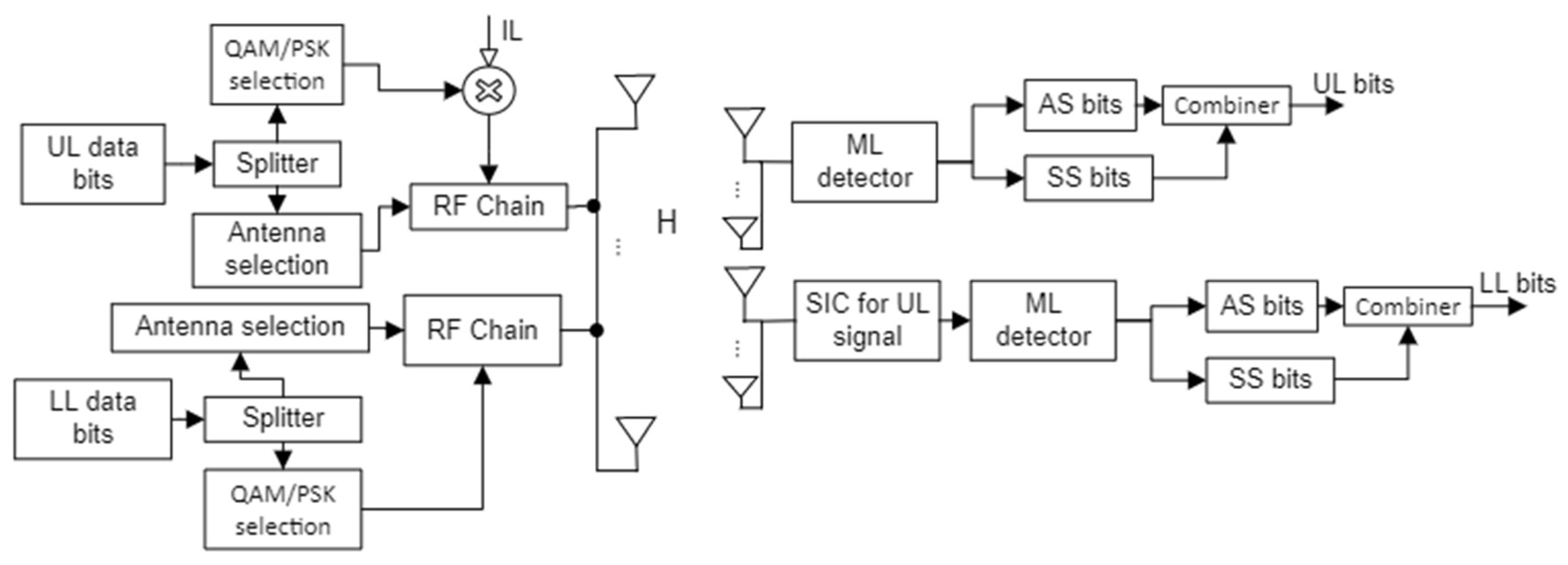
In a single-cell broadcasting network, consider a two-layer LDM downlink system. The UL and LL layers provide low and high data rate services to mobile and fixed receivers, respectively as portrayed in Figure 1. Each one of these receivers is equipped with $N_r$ receive antennas (RAs) whereas the base station (BS) employs $N_t$ transmit antennas (TAs). In conventional SM-LDM systems [12,13,14,15,16], at every transmission time, the data of each layer are split into antenna selection (AS) and symbol selection (SS) bits. The AS bits of the UL ($b_{AS}^U={\log }_2\left(N_t\right)$) specify the ith active antenna to convey the mth modulation symbol $s_m$ ($E\left[{\left|s_m\right|}^2\right]=1$) that is chosen by the SS bits ($b_{SS}^U={\log }_2\left(M_U\right)$). Similarly, the jth active antenna is determined through the AS bits of the LL ($b_{AS}^L={\log }_2\left(N_t\right)$) to transmit the nth symbol $s_n$ that is identified via the SS bits ($b_{SS}^L={\log }_2\left(M_L\right)$). Accordingly, the received signal at UL and LL receivers are given as follows:

$$\begin{gathered} {\mathit{y}}_U=\sqrt{{\rho }_U}{\mathit{h}}_i^U{s}_m+\sqrt{{\rho }_L}{\mathit{h}}_j^U{s}_n+{\mathit{w}}_U \\ {\mathit{y}}_L=\sqrt{{\beta }_L}\left(\sqrt{{\rho }_U}{\mathit{h}}_i^L{s}_m+\sqrt{{\rho }_L}{\mathit{h}}_j^L{s}_n\right)+{\mathit{w}}_L. \end{gathered}$$

(1)

where ${\mathit{h}}_i^U$ and ${\mathit{h}}_j^L$ denote the ($N_r\times 1$) column channel vectors from the (${N_r\times N}_t$) channel matrices of the UL and LL, respectively. Each component of the channel vectors can be viewed as an independently and identically distributed (i.i.d.) complex Gaussian random variable with a zero mean and unit variance. The additive white Gaussian noise (AWGN) at ULth and $LL\mathrm{t}\mathrm{h}$ receivers are, respectively, represented by ${\mathit{w}}_U$ and ${\mathit{w}}_L$; their components are i.i.d. complex Gaussian random variables with mean zero and variance ${\sigma }_0^2=1/\gamma$, where $\gamma$ is the total signal-to-noise ratio (SNR) per receive antenna at the ULth receiver. Additionally, ${\rho }_U$ and ${\rho }_L$ represent the ratio of the transmit power allocated for UL and LL, respectively, such that ${\rho }_U+{\rho }_L=1$ and the injection level is given by $IL={\rho }_U/{\rho }_L$. Low SNR thresholds of 0 dB are typical values for the ULth receiver, where it is considered to face more challenging reception conditions than the LLth receiver. Hence, ${\beta }_L$ is defined here as the SNR threshold difference ratio between UL and LL receivers. Accordingly, the total SNR at the ULth receiver is equal to ${\rho }_U\gamma$ whereas the SNR at the LLth receiver is ${{\rho }_L\beta }_L\gamma$.

Assuming perfect channel state information (CSI) at the receivers, the UL estimates its ith and mth indices to detect the transmitted AS and SS bits by applying the maximum likelihood (ML) detector as

$$\widehat{𝑖},\widehat{m}=\underset{1\le i\le N_t,1\le m\le M_U}{\underbrace{arg min}}{‖{\mathit{y}}_U-\sqrt{{\rho }_U}{\mathit{h}}_i^U{s}_m‖}^2.$$

(2)

On the other hand, the LLth receiver applies SIC to remove the interference of the ULth signal. Hence, it first estimates the ith and mth indices as

$$\widehat{i},\widehat{m}=\underset{1\le i\le N_t,1\le m\le M_U}{\underbrace{arg min}}{‖{\mathit{y}}_L-\sqrt{{\beta }_L{\rho }_U}{\mathit{h}}_i^L{s}_m‖}^2.$$

(3)

Then, the jth and nth indices of the LLth layer are estimated as

$$\widehat{j},\widehat{n}=\underset{1\le j\le N_t,1\le n\le M_L}{\underbrace{arg min}}{‖{\mathit{y}}_L-\sqrt{{\beta }_L}\left(\sqrt{{\rho }_U}{\mathit{h}}_{\widehat{i}}^L{s}_{\widehat{m}}+\sqrt{{\rho }_L}{\mathit{h}}_j^L{s}_n\right)‖}^2$$

(4)

3. Proposed Biased-Power Allocation (Bi-PA) for SM-LDM Systems

In contrast to the Preassigned-Power Allocation (Pre-PA) methods [12,13,15], this research proposes a biased-PA (Bi-PA) for the SM-LDM systems. To improve the fairness between the layers in terms of the BER performance, the ratios in the Bi-PA method are produced such that the SINRs of the UL and LL are almost identical. As explained previously, in LDM systems, the LL employs high-order modulation, and accordingly, it has a small SMED between the constellation points. The UL, on the other hand, utilizes low-order modulation with powerful SMED to accomplish strong transmission. This difference yields a significant BER performance gap between the layers. In broadcasting systems, the LL fixed receiver has a better SNR threshold than the UL mobile receiver, but it employs a higher modulation constellation which conversely deteriorates the BER performance. Additionally, this higher modulation affects the UL performance and becomes interference limited at the high SNR values and yields to an error floor problem. Accordingly, the power ratios need to be adaptively assigned.

Due to the importance and significance of the SINRs and the SMED factor, the suggested Bi-PA distributes the power ratios to obtain equal SINRs, and these SINRs take the SMED factor into mind. The UL receiver uses the ML detector in the SM-LDM receiver model described in Section 2 to estimate its information bits that are mapped to the modulation and spatial symbols, as shown in (2). The UL signal includes interference from the LL signal in addition to the AWGN with zero mean and variance ${\sigma }_0^2=1/\gamma$. Accordingly, the UL SINR is given by ${\rho }_U/({\rho }_L+1/\gamma )={\rho }_U\gamma /({\rho }_L\gamma +1)$. On the other hand, the LL receiver applies the SIC detector to first estimate and cancel the UL signal as in (3). Then, it applies the ML detector to estimate its information bits as in (4). Hence, the SINR at the LL receiver is given by ${{\beta }_{\mathrm{L}}\mathsf{\rho }}_{\mathrm{L}}/(1/\gamma )={{\beta }_{\mathrm{L}}\mathsf{\rho }}_{\mathrm{L}}\gamma$ assuming that the UL signal has been perfectly canceled. Now, we add the SMED factor to the numerator of both SINRs to include its effect. Large SMED as in UL constellations (i.e., QPSK is an example) yields higher SINR and better system performance. Low SMED as in LL constellations (i.e., 64QAM is an example) yields low SINR and bad performance. Thus, the SINRs become ${\rho }_U\gamma {\mathrm{D}}_U/({\rho }_L\gamma +1)$ and ${{\beta }_{\mathrm{L}}\mathsf{\rho }}_{\mathrm{L}}\gamma {\mathrm{D}}_L$ for UL and LL, respectively. By equating both SINRs, the closed form of power ratios can be given as

$${\rho }_L=\frac{\sqrt{{({\beta }_L{D}_L+D_U)}^2+4{\beta }_L{D}_L{D}_U\gamma }-({\beta }_L{D}_L+D_U)}{2{\beta }_L{D}_L\gamma },{\rho }_U=1-{\rho }_L.$$

(5)

From (5), the power ratios are generated such that ${\rho }_L<{\rho }_U$ and both ratios should equal 1 (${\rho }_L+{\rho }_U=1)$. Hence, the adapted ratios for UL and LL, respectively, will be $\frac{1}{2}<{\rho }_U<1$ and $0<{\rho }_L<1/2$. It can be noticed from (5) that the power ratios are produced in response to the modulation schemes ($D_L$ and $D_U$), SNR ($\gamma$), and the SNR threshold difference ratio between the layers (${\beta }_L$). In other words, the power ratios ${\rho }_L$ and ${\rho }_U$ are dynamically changed according to the mentioned parameters.

The adaptive change of the power ratios has positive advantages for both layers. The LL’s power ratio ${\rho }_L$ increases if the SMED between LL symbols ($D_L$) is low and in cases of less ${\beta }_L$ and low SNR values. Hence, at a low SNR region, the LL layer obtains a high ratio (relative to the case of Pre-PA). Because the LL applies the SIC process and becomes a noise-limited layer, the relatively high LL ratio is expected to improve its possibility of correct detection and consequently enhance its performance. Considering that ${\beta }_L$ and $D_L$ are constant, the increase of SNR yields a decrement in ${\rho }_L$. This reduction is significant to reduce the effect of LL interference on the UL receiver because the UL does not apply SIC and considers the LL signal as noise. Moreover, the low LL’s power ratio does not have a noticeable impact on its performance at the high SNR region. In contrast, the UL layer starts with a relatively small power ratio at low SNR values and then increased gradually to deal with the interference from the LL signal. Increasing the UL ratio at high SNR is also crucial for successful SIC at the LL receiver. Numerical comparison examples between the Pre-PA and Bi-PA will be given in Section 6.

4. Proposed SAS-Based SM-LDM System Model

In the typical SM-LDM system outlined in Section 2, each layer makes its own independent choice about which active transmit antenna to use. It increases SE but requires two RF chains (considering two layers UL and LL), which lowers EE and adds hardware complexity. It makes it harder for receivers to identify each layer’s active antenna. Additionally, it requires SIC for the LL signal and increases ILI considering that every layer transmits a modulation symbol. To overcome these problems, we propose a new technique called shared antenna selection (SAS) to activate only one antenna per transmission time which yields to transmit a unique modulation symbol from both layers. The decision of choosing which antenna is active is determined cooperatively via UL and LL. More specifically, the whole data of the UL are combined with the AS bits of the LL layer to determine the active antenna as shown in Figure 2. Hence, $b_{AS}^U+b_{AS}^L={\log }_2\left(N_t\right)$, and $b_{SS}^L={\log }_2\left(M_L\right)$. It can be noticed here that one active antenna requires a single RF chain which improves the EE and reduces the hardware complexity. This will be more incredible for multiple layers of SM-LDM, especially with many antennas at the transmitter. In addition, the UL delivers its service completely through implicit modulation of the spatial domain; there is no modulation symbol transmitted. Hence, it conveys an SSK signal which offers several features. Firstly, there is no need for the SIC process at the LL receiver which reduces the complexity of the whole system and alleviates the problem of SIC propagation error. Secondly, the total power is allocated to the LL signal. Accordingly, it is free from optimizing the power allocation and finding suitable ratios. Additionally, assigning the full power to the transmitted symbol of the LL signal yields reinforcement of the possibility of successful detection of both LL and UL bits. Thirdly, there is no ILI which is expected to yield better system performance.

An additional advantage of the SAS technique comes from the flexibility to deliver the LL service through both spatial (i.e., AS bits) and modulation symbols (i.e., SS bits). More specifically, sharing the decision of antenna selection provides more freedom to convey the services via AS bits. This allows utilizing the case of a higher number of antennas more efficiently; increasing $N_t$ leads to more AS bits for the LL which decreases the SS bits, and consequently there is less modulation constellation size. Therefore, it relieves the interference and consequently provides better BER performance.

Assume that a cth common antenna is activated through the combined AS bits from both layers’ data and the LLth modulation symbol $s_l$ is selected by the SS bits ($b_{SS}^L$). Hence, the received signal at the UL and LL receivers are given as follows:

$$\begin{gathered} {\mathit{y}}_U={\mathit{h}}_c^U{s}_l+{\mathit{w}}_U. \\ {\mathit{y}}_L=\sqrt{{\beta }_L}{\mathit{h}}_c^L{s}_l+{\mathit{w}}_L. \end{gathered}$$

(6)

where the channel vector between the shared active $c\mathrm{t}\mathrm{h}$ antenna and the ULth and LLth receivers is denoted by ${\mathit{h}}_c^U$ and ${\mathit{h}}_c^L$, respectively. All elements of the vector ${\mathit{h}}_c^U$ and ${\mathit{h}}_c^L$ are i.i.d. complex Gaussian random variables with zero mean and unit variance. As shown in Figure 2, the ULth receiver applies the ML detector to estimate the index of the active transmit antenna as follows:

$$\widehat{c}=\underset{1\le c\le N_t,1\le l\le M_L}{\underbrace{arg min}}{‖{\mathit{y}}_U-{\mathit{h}}_c^U{s}_l‖}^2.$$

(7)

From the estimated index $\widehat{c}$ the AS bits of UL are obtained. After that, the LLth receiver estimates the modulation symbol as follows:

$$\widehat{l}=\underset{1\le c\le N_t,1\le l\le M_L}{\underbrace{arg min}}{‖{\mathit{y}}_L-{\mathit{h}}_c^L{s}_l‖}^2.$$

(8)

Hence, the LL bits are acquired from the estimated index $\widehat{l}$.

5. Spectral Efficiency (SE) Analysis for SAS-Based SM-LDM

This section introduces the SE analysis of both layers in the SM-LDM system model that applies the proposed SAS technique. Finite alphabet inputs (modulation and spatial symbols) are employed. Assume perfect channel estimation at the receivers and that the modulation symbol constellation of the LL receiver is known for both receivers. For the analysis, we define the spatial constellation spaces for UL and LL, respectively, as ${\mathcal{H}}_U=\left\{{\mathit{h}}_1^U,{\mathit{h}}_2^U,{\mathit{h}}_c^U,\dots ,{\mathit{h}}_{N_t}^U\right\}$ and ${\mathcal{H}}_L=\left\{{\mathit{h}}_1^L,{\mathit{h}}_2^L,{\mathit{h}}_c^L,\dots ,{\mathit{h}}_{N_t}^L\right\}$ with $N_t$ spatial symbols. Likewise, the signal space for LL with $M_L$ signal symbols is denoted as ${\mathcal{S}}_L=\left\{s_1^L,s_2^L,s_l^L,\dots ,s_{M_L}^L\right\}$. The SE for each layer can be calculated by determining the mutual information (MI) obtained between the received signal, which is given in Equation (6), and the inputs from both the spatial domain for the UL (i.e., $I\left({\mathcal{H}}_U;{\mathit{y}}_U\right)$) and the signal domain as well as the spatial domain for the LL (i.e., $I({\mathcal{H}}_L,{\mathcal{S}}_L;{\mathit{y}}_L)$) [27,28].

Within the context of the proposed SAS-based SM-LDM, each layer contributes to the process of selecting the common TA in which the AS bits are mapped to a shared spatial symbol. As a result, the MI produced by spatial symbols for each layer is determined by the layer’s AS bit allocation. These bits split the $N_t$ antennas into groups $G_U=2^{b_{AS}^U}$ and $G_L=2^{b_{AS}^L}$; each group includes several indices equal to $I_U=N_t/G_U$ and $I_L=N_t/G_L$. An example of this AS bits mapping is provided in Appendix A. The spatial constellation of the UL becomes ${\mathcal{H}}_U=\left\{{\mathit{h}}_{\mathrm{1,1}}^U,{\mathit{h}}_{g\left(U\right),i\left(U\right)}^U,\dots ,{\mathit{h}}_{G_U,I_U}^U\right\}$ where $g\left(U\right)$ is the group index (i.e.,$g\left(U\right)\in \left\{1,\dots ,G_U\right\}$) and $i\left(U\right)$ is the antenna index per group (i.e., $i\left(U\right)\in \left\{1,\dots ,I_U\right\}$). Accordingly, ${\mathit{h}}_{g\left(U\right),i\left(U\right)}^U$ represents the spatial symbol transmitted by UL. Similarly, ${\mathit{h}}_{g\left(L\right),i\left(L\right)}^L$ is the spatial symbol transmitted by the LL. At specific transmission time, the AS bits of the UL yield a group index $g$, whereas the AS bits of the LL specify the index i. Hence, the received signals shown in (6) can be reformed as follows:

$$\begin{gathered} {\mathit{y}}_U={\mathit{h}}_{g,i}^U{s}_l+{\mathit{w}}_U. \\ {\mathit{y}}_L=\sqrt{{\beta }_L}{\mathit{h}}_{g,i}^L{s}_l+{\mathit{w}}_L. \end{gathered}$$

(9)

The sum-rate of the SAS-based SM-LDM system can be evaluated as follows:

$$R_{Sum}=I\left({\mathcal{H}}_U;{\mathit{y}}_U\right)+I\left({\mathcal{H}}_L,{\mathcal{S}}_L;{\mathit{y}}_L\right)$$

(10)

where $I\left({\mathcal{H}}_U;{\mathit{y}}_U\right)$ is the MI gained from the UL (SSK layer). The second term $I\left({\mathcal{H}}_L,{\mathcal{S}}_L;{\mathit{y}}_L\right)$ is the joint MI realized from both spatial and modulation symbols transmitted by LL.

5.1. SE of Upper Layer

For UL, the MI is measured between the discrete channel input and continuous output which can be given as follows [29]:

$$I\left({\mathcal{H}}_U;{\mathit{y}}_U\right)=E_{{\mathit{h}}_g^U,{\mathit{y}}_U}\left[{\log }_{2}p\left({\mathit{y}}_U|{\mathit{h}}_g^U\right)/p\left({\mathit{y}}_U\right)\right]=\sum _{g=1}^{G_{UL}}\int p({\mathit{h}}_g^U)p\left({\mathit{y}}_U|{\mathit{h}}_g^U\right){\log }_2\frac{p\left({\mathit{y}}_U|{\mathit{h}}_g^U\right)}{p\left({\mathit{y}}_U\right)}d{\mathit{y}}_U,$$

(11)

where $p\left({\mathit{h}}_g^U\right)=1/G_U$ reflects with equal probability the spatial symbol ${\mathit{h}}_g^U$ supplied by UL. Additionally, in (9), $p\left({\mathit{y}}_U\right)$ is the probability density function (PDF) of the received vector ${\mathit{y}}_U$, and $p\left({\mathit{y}}_U|{\mathit{h}}_g^U\right)$ is the conditional PDF, assuming that UL selects the spatial symbol ${\mathit{h}}_g^U$. Accordingly, (11) can be rewritten as

$$I\left({\mathcal{H}}_U;{\mathit{y}}_U\right)=\frac{1}{G_U}\sum _{g=1}^{G_U}\int p\left({\mathit{y}}_U|{\mathit{h}}_g^U\right){\log }_2\frac{p\left({\mathit{y}}_U|{\mathit{h}}_g^U\right)}{\frac{1}{G_U}{\sum }_{m=1}^{G_U}p\left({\mathit{y}}_U|{\mathit{h}}_m^U\right)}d{\mathit{y}}_U,$$

(12)

Which can be simplified to

$$I\left({\mathcal{H}}_U;{\mathit{y}}_U\right)={\log }_2{G}_U-\frac{1}{G_U}\sum _{g=1}^{G_U}\int p\left({\mathit{y}}_U|{\mathit{h}}_g^U\right){\log }_2\left[1+\frac{\sum _{m=1,\ne g}^{G_U}p\left({\mathit{y}}_U|{\mathit{h}}_m^U\right)}{p\left({\mathit{y}}_U|{\mathit{h}}_g^U\right)}\right]d{\mathit{y}}_U.$$

(13)

Because a closed-form formula for $I\left({\mathcal{H}}_U;{\mathit{y}}_U\right)$ is difficult to identify, the Monte Carlo (MC) integration is utilized to compute it in Equation (13) [30]. The expression $I\left({\mathcal{H}}_U;{\mathit{y}}_U\right)$ can be represented as follows in the form of expectations:

$$I\left({\mathcal{H}}_U;{\mathit{y}}_U\right)\approx {\log }_2{G}_U-\frac{1}{G_U}\sum _{g=1}^{G_U}{E}_{y_U|{\mathcal{H}}_U}\left[{\log }_2\left(1+\frac{\sum _{m=1,\ne g}^{G_U}p\left({\mathit{y}}_U|{\mathit{h}}_m^U\right)}{p\left({\mathit{y}}_U|{\mathit{h}}_g^U\right)}\right)\right].$$

(14)

A significant number (let us say S) of independent random samples is collected from the signal that was received (9) to evaluate (14) [31]. This approach is used for all S transmission channels, and the estimated values obtained are averaged to provide the resultant value:

$$I\left({\mathcal{H}}_U;{\mathit{y}}_U\right)\approx {\log }_2{G}_U-\frac{1}{G_{U}S}\sum _{g=1}^{G_U}\sum _{s=1}^S{\log }_2\left[1+\frac{\sum _{m=1,\ne g}^{G_U}p\left({\mathit{y}}_U^s|{\mathit{h}}_m^U\right)}{p\left({\mathit{y}}_U^s|{\mathit{h}}_g^U\right)}\right].$$

(15)

In Equation (15), ${\mathit{y}}_U^s$ is a unique identifier for the received signal ${\mathit{y}}_U$, which is described in (9). $p\left({\mathit{y}}_U^s|{\mathit{h}}_g^U\right)$ also signifies that the $g\mathrm{t}\mathrm{h}$ group was active and the UL signal was transmitted from any of the ith antennas in the $g\mathrm{t}\mathrm{h}$ group. This probability is related to all transmission probabilities from other antennas in other groups via $p\left({\mathit{y}}_U^s|{\mathit{h}}_m^U\right)$, where $m\ne n$. Consequently, $p\left({\mathit{y}}_U^s|{\mathit{h}}_g^U\right)$ can be rewritten as:

$$p\left({\mathit{y}}_U^s|{\mathit{h}}_g^U\right)=\frac{1}{I_U}\sum _{i=1}^{I_U}p\left({\mathit{y}}_U^s|{\mathit{h}}_{g,i}^U\right),$$

(16)

Therefore, (15) can be rearranged to

$$I\left({\mathcal{H}}_U;y_U\right)\approx {\log }_2{G}_U-\frac{1}{G_{U}S}\sum _{g=1}^{G_U}\sum _{s=1}^S{\log }_2\left[1+\frac{\sum _{\begin{array}{c}m=1,\\ \ne g\end{array}}^{G_U}\sum _{ii=1}^{I_U}p\left(y_U^s\right|h_{m,ii}^U)}{{\sum }_{i=1}^{I_U}p\left(y_U^s\right|h_{g,i}^U)}\right]$$

(17)

Additionally, $p\left({\mathit{y}}_U^s\right|{\mathit{h}}_{g,i}^U)$ is given by:

$$p(y_U^s|h_{g,i}^U)=\frac{1}{{\pi }^{N_r}\left|{\mathit{\Gamma }}_U\right|}\exp \left\{-{{\mathit{y}}_U}^H{{\mathit{\Gamma }}_U}^{-1}{\mathit{y}}_U\right\},$$

(18)

where ${\mathit{\Gamma }}_U={\mathit{h}}_{g,i}^U{\left({\mathit{h}}_{g,i}^U\right)}^H+{\sigma }_0^2\mathit{I}$ represents the non-singular covariance matrix.

5.2. SE of Lower Layer

Now shifting to the LL, $I\left({\mathcal{H}}_L,{\mathcal{S}}_L;{\mathit{y}}_L\right)$ is the achievable rate (mutual information) between the continuous received signal and discrete symbols (spatial and modulation) of the LL which is given by [28,29]:

$$I\left({\mathcal{H}}_L,{\mathcal{S}}_L;{\mathit{y}}_L\right)=\sum _{g=1}^{G_L}\sum _{l=1}^{M_L}p({\mathit{h}}_g^L,s_l^L)\left[\int p\left({\mathit{y}}_L|s_l^L,{\mathit{h}}_g^L\right){\log }_2\frac{p\left({\mathit{y}}_L|s_l^L,{\mathit{h}}_g^L\right)}{p\left({\mathit{y}}_L\right)}\right]d{\mathit{y}}_L,$$

(19)

where LL’s signal and spatial symbols are denoted by $s_l^L$ and ${\mathit{h}}_g^L$, respectively. When ${\mathit{h}}_g^L$ and $s_l^L$ are chosen as the spatial and signal symbols, respectively, the conditional PDF of the received vector is $p\left({\mathit{y}}_L|{s_l^L,\mathit{h}}_g^L\right)$. The joint probability is denoted by $p({\mathit{h}}_g^L,s_l^L)=1/G_L{M}_L$, and Equation (19) can be rewritten as:

$$I\left({\mathcal{H}}_L,{\mathcal{S}}_L;{\mathit{y}}_L\right)=\frac{1}{G_L{M}_L}\sum _{g=1}^{G_L}\sum _{l=1}^{M_L}\int p\left({\mathit{y}}_L|s_l^L,{\mathit{h}}_g^L\right){\log }_2\frac{p\left({\mathit{y}}_L|s_l^L,{\mathit{h}}_g^L\right)}{\frac{1}{G_L{M}_L}\sum _{m=1}^{G_L}{\sum }_{n=1}^{M_L}p\left({\mathit{y}}_L|s_n^L,{\mathit{h}}_m^L\right)}d{\mathit{y}}_L,$$

(20)

It is also challenging to find a closed formula for (20); thus, we use MC integration to obtain:

$$I\left({\mathcal{H}}_L,{\mathcal{S}}_L;{\mathit{y}}_L\right)\approx {\log }_2\left(G_L{M}_L\right)+\frac{1}{G_L{M}_{L}S}\sum _{g=1}^{G_L}\sum _{l=1}^{M_L}\sum _{s=1}^S{\mathit{log}}_2\frac{p\left(y_L^s|s_l^L,{\mathit{h}}_g^L\right)}{\sum _{m=1}^{G_L}\sum _{n=1}^{M_L}p\left(y_L^s|s_n^L,{\mathit{h}}_m^L\right)},$$

(21)

Rearranging (21), it yields:

$$I\left({\mathcal{H}}_L,{\mathcal{S}}_L;{\mathit{y}}_L\right)\approx {\log }_2\left(G_L{M}_L\right)-\frac{1}{G_L{M}_{L}S}\sum _{g=1}^{G_L}\sum _{l=1}^{M_L}\sum _{s=1}^S{\log }_2\left[1+\sum _{\begin{array}{c}m=1,\\ \ne g\end{array}}^{G_L}\sum _{n=1}^{M_L}\frac{p\left({\mathit{y}}_L^s|s_n^L,{\mathit{h}}_m^L\right)}{p\left({\mathit{y}}_L^s|s_l^L,{\mathit{h}}_g^L\right)}\right]$$

(22)

The PDF $p\left({\mathit{y}}_L^s|s_l^L,{\mathit{h}}_g^L\right)$ can be rewritten by taking into consideration the $i\mathrm{t}\mathrm{h}$ index of the TA among the $g\mathrm{t}\mathrm{h}$ group antennas, and it can be given as follows:

$$p\left({\mathit{y}}_L^s|s_l^L,{\mathit{h}}_g^L\right)=\frac{1}{I_k}{\sum }_{i=1}^{I_k}p\left({\mathit{y}}_k|s_l^L,{\mathit{h}}_{g,i}^L\right)$$

(23)

Hence, (17) can be reformulated as

$$I\left({\mathcal{H}}_L,{\mathcal{S}}_L;{\mathit{y}}_L\right)\approx {\mathit{log}}_2\left(G_L{M}_L\right)-\frac{1}{G_{L}MS}\sum _{g=1}^{G_L}\sum _{l=1}^{M_L}\sum _{s=1}^S{\mathit{log}}_2\left[1+\sum _{\begin{array}{c}m=1,\\ \ne g\end{array}}^{G_L}\sum _{ii=1}^{I_L}\sum _{n=1}^{M_L}\frac{p\left({\mathit{y}}_L^s|s_n^L,{\mathit{h}}_{m,ii}^L\right)}{\sum _{i=1}^{I_L}p\left({\mathit{y}}_L^s|s_l^L,{\mathit{h}}_{g,i}^L\right)}\right]$$

(24)

In (24), On the right-hand side, the first term represents the highest rate that may be achieved using LL. The conditional PDF $p\left({\mathit{y}}_L^s|s_l^L,{\mathit{h}}_{g,i}^L\right)$ is expressed as

$$p\left({\mathit{y}}_L^s|s_l^L,{\mathit{h}}_{g,i}^L\right)=\frac{{\pi }^{-N_r}}{\left|{\mathit{\psi }}_L\right|}\exp \left\{-{\left({\mathit{y}}_L^s-\sqrt{{\beta }_L}{s}_l^L{\mathit{h}}_{g,i}^L\right)}^H{\left({\mathit{\psi }}_L\right)}^{-1}\left({\mathit{y}}_L^s-\sqrt{{\beta }_L}{s}_l^L{\mathit{h}}_{g,i}^L\right)\right\}$$

(25)

where ${\mathit{\psi }}_L={\beta }_L{\mathit{h}}_{g,i}^L{\left({\mathit{h}}_{g,i}^L\right)}^H+{\sigma }_0^2\mathit{I}$ represents the covariance matrix.

6. Results and Discussion

This part presents the numerical results for the proposed Bi-PA and SAS approaches. Three cases are employed for the Pre-PA: $IL\left(\mathrm{d}\mathrm{B}\right)=6,9.54$, and $12.8$ for Case 1, Case 2, and Case 3. In comparison, the proposed Bi-PA changes the power ratios adaptively. Classic SM-LDM without SAS is abbreviated as SM-LDM, whereas the proposed SAS-based SM-LDM is abbreviated as SAS-SM-LDM. 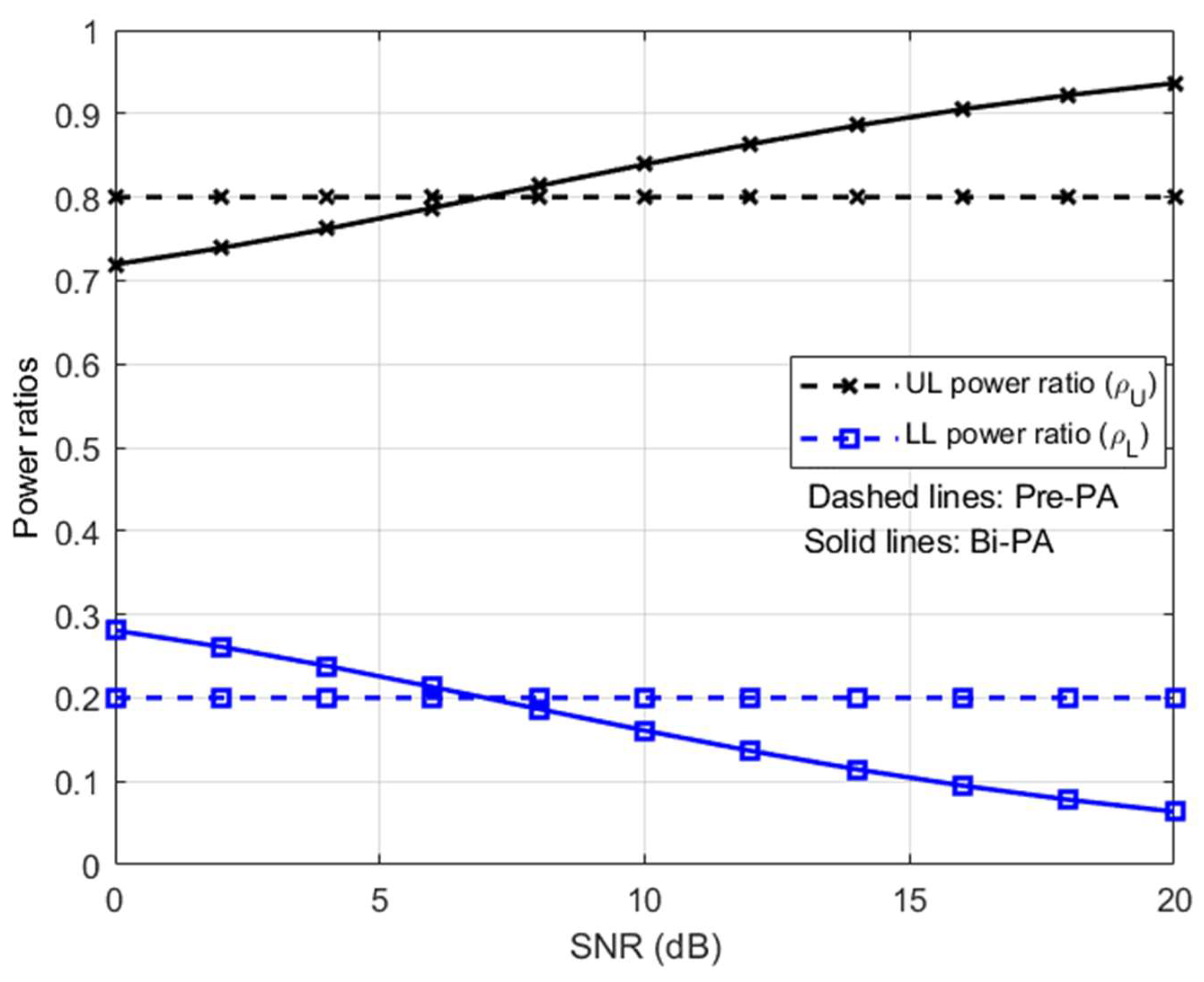Figure 3 shows the power ratios versus the SNR generated using Pre-PA and Bi-PA for LL and UL in SM-LDM systems where $N_t=N_r=4$, and select QPSK for UL and 16-QAM for LL. The UL information bits select an antenna to convey its QPSK symbol. Similarly, the LL bits transmitted are mapped to the active antenna and 16-QAM symbols. In Pre-PA, the power ratios assigned to each symbol are fixed to ${\rho }_U=0.8$ and ${\rho }_L=0.2$. Alternatively, as shown in the results of Figure 3, the ratios are adaptively changed with the SNR. Referred to Equation (5), ${\rho }_L$ decreases along with the increase of SNR while ${\rho }_U$ increased. Furthermore, the results show that the power ratio thresholds for both layers are satisfied where $0<{\rho }_L\le 1/2$ and $\frac{1}{2}<{\rho }_U<1$.

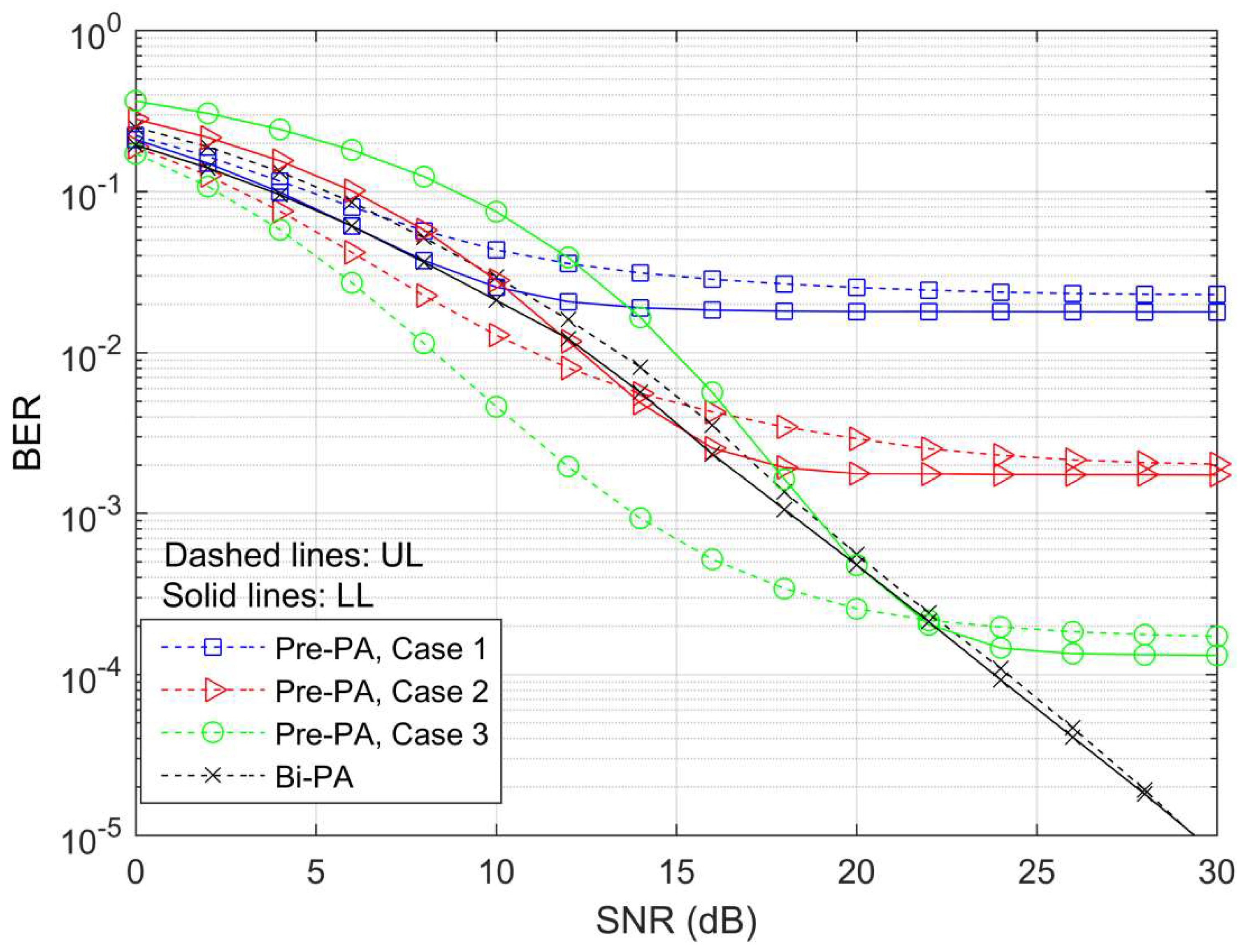
The BER of two layers of the SM-LDM system is depicted in Figure 4 when the Pre-PA and proposed Bi-PA methods are used. We set $N_t=N_r=4$, and select QPSK for UL and 16-QAM for LL. Given this configuration, the IL ratios for the Bi-PA are adaptively changing with the SINR and given as follows: [4.0850 4.5149 5.0474 5.6769 6.3909 7.1742 8.0116 8.8901 9.7993 10.7310 11.6795] $\mathrm{d}\mathrm{B}$. The results show that the Pre-PA cases suffer from BER floor problems at high SNR. Additionally, increasing the IL ratio decreases the UL BER at low and medium SNR, but it increases the LL BER. On the other hand, the results demonstrate that the proposed Bi-PA solves the error floor problem and provides better fairness between the layers. It is worth noting here that the Bi-PA adaptively allocates the power ratios based on equalizing the SINRs for both layers. Hence, the ratios are continuously specified such that the BER of UL and LL is nearly identical. This enhances fairness and simultaneously finds the appropriate ratios even though the SNR and interference are varying.

In Figure 5, the SE results are shown for the case of two layers and the configuration is identical to Figure 4. For clarity, only two cases are shown for the Pre-PA. Note that the transmission rate of the layers is ${UL}^{TR}=4 \mathrm{b}\mathrm{i}\mathrm{t}\mathrm{s}/\mathrm{s}/\mathrm{H}\mathrm{z}$, ${LL}^{TR}=6 \mathrm{b}\mathrm{i}\mathrm{t}\mathrm{s}/\mathrm{s}/\mathrm{H}\mathrm{z}$. Firstly, by investigating the Pre-PA cases, it can be noticed that the UL rate is relatively improved particularly at low and medium SNR values via increasing the IL ratio as in Case 2 compared to Case 1. However, this could affect the capability of the LL receiver to correctly estimate its information which negatively affects the achievable LL rate and consequently the Sum-rate. On the other hand, the adaptive and dynamic change of the power ratios in the Bi-PA enhances the achievable LL rate and the Sum-rate, especially at the low and intermediate SNR regions.

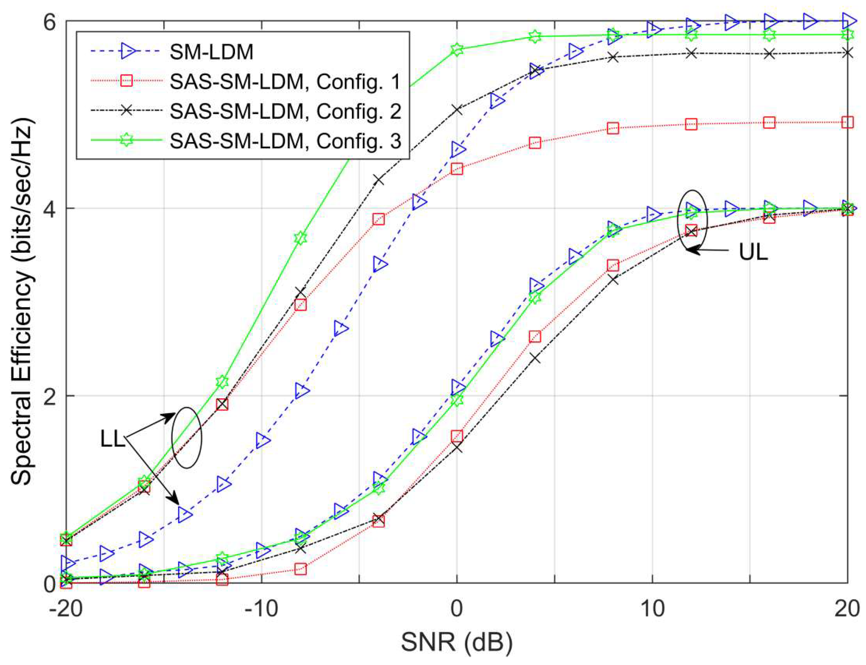
The following Figure 6, Figure 7 and Figure 8 evaluate the proposed SAS technique in terms of SE and BER. Note that the Bi-PA is applied in all cases. The layers rates and the sum-rate are shown, respectively, in Figure 6 and Figure 7. As described in the caption of the figures, the transmission rates (TRs) of the layers are $U{L}^{TR}=4 \mathrm{b}\mathrm{i}\mathrm{t}\mathrm{s}/\mathrm{s}/\mathrm{H}\mathrm{z}$ and $L{L}^{TR}=6 \mathrm{b}\mathrm{i}\mathrm{t}\mathrm{s}/\mathrm{s}/\mathrm{H}\mathrm{z}$. The SM-LDM applies $N_t$ = 4, QPSK, and 16-QAM, respectively, for UL and LL. For SAS-SM-LDM, recall that UL bits (i.e., ${\log }_2{N}_t$) select the active antenna among $N_t$; hence, it applies an SSK signal, and no modulation symbol is transmitted. On the other hand, the LL conveys a modulation symbol chosen from $M_L$ constellation. Three configurations are examined here where the spatial and modulation constellation sizes are varied. Referring to the captions, the spatial bits (i.e., ${\log }_2{N}_t$) are shared between UL and LL.

Among the arrangements, the results reveal that increasing $N_t$ provides higher rates and sum-rate than increasing $M_L$. For example, 16-QAM for LL and $N_t=64$ in Config. 2 offer higher rates, particularly for LL at medium and high SNR regions than 64-QAM for LL and $N_t=16$ in Config. 1. Similarly, 8-PSK for LL and $N_t=128$ in Config. 3 deliver further improvement compared to Config. 1 and Config. 2. Furthermore, it is worth noting here that all SAS-SM-LDM models provide a high rate for UL and sum-rate than SM-LDM at low and medium SNR values. Moreover, conveying more spatial bits than the modulation bits in the SAS-SM-LDM systems allows for maximization of the gain at low and medium SNR and simultaneously minimizes the performance gap relative to the SM-LDM at high SNR values. These spatial bits mapped from the LL user led to a higher achievable rate at the LL receiver for low and intermediate SNR values. The increased likelihood of correct detection for spatial bits in noise-limited regions is consistent with this finding, as reported in the SM literature. In addition, at high SNR values, the impact of LL’s interference on the UL interference-limited user has been mitigated thanks to the reduction of LL’s modulation order and the implicit conveyance of spatial bits.

The BER comparison between the SM-LDM and SM-LDM-SAS is shown in Figure 8. The same configuration as in Figure 7 is used here. As can be seen, the SM-LDM layers have nearly identical BERs because of the Bi-PA. The results then confirm that the proposed SAS technique allows for greater flexibility and utilization of the spatial domain, resulting in an overall BER improvement for both UL and LL. Increasing the number of antennas in the various SAS configurations also reduces the BER. Furthermore, after $SNR>12 \mathrm{d}\mathrm{B}$, the results show that the SM-LDM-SAS with Config. 3 provides the best BER performance for both layers. It is caused by implicitly modulating all of UL’s information bits in the spatial domain. Furthermore, the sharing property allows for a reduction in the QAM/PSK constellation size of LL, which reduces ILI and allows for better detection of the LL bits.

7. Conclusions

This study proposed biased-power allocation (Bi-PA) and shared antenna selection (SAS) algorithms intending to improve the performance of SM-LDM systems. The proposed Bi-PA adaptively adjusted power ratios based on signal-to-interference-plus-noise ratios (SINRs) and squared minimum Euclidean distances (SMEDs) between modulation constellations to improve BER fairness, eliminate the error floor problem, and achieve nearly identical BERs for both layers. SAS simplifies the SM-LDM system by allowing diverse layers to cooperate on antenna selection, increasing the sum-rate while simultaneously enhancing BER performance and fairness. According to the BER results, the SAS provides gains ranging from 7 to 15 dB for LL, while UL performance ranges from slight gain to minor loss. The numerical findings demonstrated the advantages of the Bi-PA and SAS methods, such as higher achievable rates, sum-rate, spectral efficiency, and reduced inter-layer interference. By utilizing the benefits of SM, SAS, and Bi-PA, our proposed system satisfies the rigorous SWaP-C reduction criteria for a MIMO RF front-end. These findings show the potential of the proposed strategies for improving the efficiency, fairness, and BER performance of SM-LDM systems in broadcasting scenarios. Although our study considers that the Bi-PA is compatible with various RF chain architectures, future work could focus on investigating the optimal RF chain architecture designs for SM-LDM systems. It could consider things such as power consumption, hardware complexity, and compatibility with emerging technologies.