Improved BIGRU Model and Its Application in Stock Price Forecasting

Abstract

In order to obtain better prediction results, this paper combines improved complete ensemble EMD (ICEEMDAN) and the whale algorithm of multi-objective optimization (MOWOA) to improve the bidirectional gated recurrent unit (BIGRU), which makes full use of original complex stock price time series data and improves the hyperparameters of the BIGRU network. To address the problem that BIGRU cannot make full use of the stationary data, the original sequence data are processed using the ICEEMDAN decomposition algorithm to derive the non-stationary and stationary parts of the data and modeled with the BIGRU and the autoregressive integrated moving average model (ARIMA), respectively. The modeling process introduces a whale algorithm for multi-objective optimization, which improves the probability of finding the best combination of parameter vectors. The ${\mathrm{R}}^2$, MAPE, MSE, MAE, and RMSE values of the BIGRU algorithm, ICEEMDAN-BIGRU algorithm, MOWOA-BIGRU algorithm, and the improved algorithm were compared. An average improvement of 14.4% over the original algorithm’s goodness-of-fit value will greatly improve the accuracy of stock price predictions.

1. Introduction

The finance market has a pivotal role, exerting a significant impact on the global macroeconomic landscape. In recent times, the increasing growth and prominence of the stock market have garnered substantial attention within the economy. Fluctuations in stock prices are influenced by a myriad of factors, including the present and future valuation of companies, macroeconomic integration, industry dynamics, historical patterns, and more. Moreover, stock data exhibit nonlinear characteristics, substantial volatility, and intricate complexities, thereby posing a formidable challenge for stock price forecasting. Nonetheless, accurate predictions in the stock market can yield valuable insights, enabling investors to mitigate their risks and capitalize on lucrative opportunities. By successfully anticipating stock market trends, investors can generate profits with minimal risk exposure and secure positive returns at lower costs. Consequently, despite the formidable nature of stock price prediction, it remains a subject of great interest among both investors and scholars alike.

Various methods have been employed to predict stock prices, including traditional econometric techniques and deep learning approaches. Commonly utilized econometric methods include autoregressive moving averages (ARMA) [1], autoregressive integrated moving averages (ARIMA) [2], and generalized autoregressive conditional heteroscedasticity (GARCH) [3]. ARMA combines the impact of previous lags (AR) and the error term (MA) to forecast future stock prices. ARIMA, an extension of ARMA, incorporates differencing as an additional factor. GARCH, on the other hand, addresses the issue of heteroscedasticity. However, these traditional econometric methods are primarily effective for stationary series and encounter challenges when handling non-stationary data.

Deep learning methodologies have been more frequently employed to predict stock prices as a result of the development of neural networks, which were more suited for non-stationary sequences. Initially, methods such as artificial neural networks (ANN), back propagation neural networks (BPNN), multilayer perceptron (MLP), and so on performed well on the issue of stock price prediction. However, these methods are not specifically for sequence data and lose time information. Unlike ANN, BPNN, and MLP, recurrent neural networks (RNNs) had feedback connections inside the neural network to learn temporal patterns. Therefore, RNNs and their variants have become the most widely used methods to predict stock prices. RNNs encounter the problem of gradient disappearance or gradient explosion when processing long-term data. To solve this problem, several variants of RNNs have emerged, including LSTM, GRU, bidirectional LSTM, bidirectional GRU, etc. [4]

BIGRU (bidirectional gated recurrent unit) is a recurrent neural network structure capable of capturing contextual information because it uses both forward and reverse temporal order and can efficiently handle long-range dependencies [5].

The current research trend is focused on leveraging hybrid models to enhance the predictive capabilities of models. The objective is to combine the strengths of multiple algorithms while mitigating the impact of their respective weaknesses on the results. Several fusion strategies have been proposed, including the fusion of neural network models (such as CNN-LSTM), ensemble model fusion techniques (such as stacking and bagging), and the integration of data decomposition algorithms (such as WT, EMD, and VMD). Data decomposition techniques are typically employed during the data preparation stage to enhance data stability. However, research on fusion models integrating these procedures is still relatively scarce.

In this study, a solution is proposed to address the issue of the limited accuracy in handling stationary data by the BIGRU model. The ICEEMDAN algorithm is utilized to separate stationary and non-stationary information in stock price time series data prior to model training. The non-stationary and stationary components of the data are modeled using BIGRU and ARIMA models, respectively. To enhance the search for the optimal set of parameter vectors, the multi-objective improvement whale algorithm is introduced. By optimizing the BIGRU algorithm, the impact of stationary information in the stock price series data on the overall performance is reduced, along with a decreased reliance on hyperparameters. This approach significantly improves the prediction accuracy of stock price time series data.

2. Related Works

2.1. Decomposition of Time Series Data

Decomposition hybrid methods in time series forecasting include decomposition models and forecasting models, and relevant studies based on these models are summarized as follows:

Norden E. Huang [6] first introduced the idea of decomposition and proposed a new method for adaptive and efficient decomposition of complex data (EMD), which introduces the local features of the signal into the eigenmode function, and the result is expressed in the form of a energy–frequency–time distribution called a Hilbert spectrum. The example proves that the method can analyze nonlinear non-stationary data well. JIA-RONG YEH [7] proposed an improved algorithm for a noise-enhanced data analysis method (CEEMD), which solves the noise pollution problem by adding positive and negative pairwise auxiliary noise, but also eliminates redundant noise to a large extent. Maria E. Torres [8] proposed a fully adaptive noisy ensemble empirical modal decomposition algorithm (CEEMDAN) based on EEMD, which adds appropriate white noise in the first screening stage and continues adding white noise to the subsequent decomposed modes, reducing the computational cost, but some interference signals may appear in the early stage. Marcelo A. Colominas [9] improved CEEMDAN by proposing ICEEMDAN to select the kth IMF component of the white noise decomposed by EMD to join the white noise and obtain a model with less noise and more physical significance. The results of Yu-jie Xiao [10,11] and Mohanad S. AL-Musaylh [12] showed that the prediction accuracy of the hybrid algorithm based on ICEEMDAN decomposition is better than that of the hybrid models of other decomposition algorithms.

To predict a decomposed time series, many studies also have a different structure. Yang [13] used ARIMA to analyze the linear part of the data and EMD to process the nonlinear part of the decomposed time series into SVR, and finally established a comprehensive model combining ARIMA, EMD, and SVR and selected four groups of stocks for experimental validation. Buyuksahin [14] proposed a hybrid ARIMA-ANN algorithm by combining ARIMA with an ANN using the EMD technique, with the experimental results showing that the hybrid algorithm with EMD decomposition has better performance than the traditional hybrid algorithm and single model. Rezaei [15] extracted financial data depth features and established CEEMD-CNN-LSTM and EMD-CNN-LSTM hybrid algorithms, and the experimental results show that CEEMD has a better prediction effect compared to EMD. Zhang [16] combined MLP and RNN with ARIMA, respectively, to build ARIMA-MLP and ARIMA-RNN hybrid models, and validated them on three sets of stock data. The results all showed that the hybrid models have stronger robustness than the individual models. Cheng [17] used CEEMD to decompose crude oil price data and obtained structural breaks using ICSS and the Chow test, and combined the decomposed data and structural breaks to build a CEEMD-ARIMA-SVM model, which experimentally proved that the hybrid model has better results in dealing with complex data and can be used in many fields.

2.2. BIGRU

GRUs are a simpler variant of a recurrent neural network of an LSTM network. GRUs have fewer parameters, less computational overhead for training, and a faster training speed. GRUs and BIGRUs have been studied extensively in sequence prediction.

She [18] proposed a bootstrap-based method for predicting RUL for BIGRUs that is of great importance in practical manufacturing. Zhang [19] used BIGRUs to extract information and a mixed BIGRU with MMoE to construct a dual-task network structure for industrial equipment evaluation and prediction, and the simulation verified the excellent accuracy of the method. Guo [20] used GRUs to discover the correlation between time series and established a GRU-based Gaussian mixture VAE system (GGM-VAE) for anomaly testing, which was experimentally proven to be superior to existing anomaly testing methods. Li [21] proposed a new framework combining a BIGRU and an SSA by exploiting the feature that BIGRUs can make full use of the information in production sequences and correlation features. The accuracy and robustness of the method were proven to be better than other models in the example analysis.

Zhu [22] found that the VMD-BIGRU model outperformed GRUs and LSTM in predicting high returns when constructing a comprehensive financial investment decision system. Wang [23] tested a combination optimization model using BiLSTM and BIGRUs for simultaneous prediction on four stock groups, demonstrating superior performance compared to other benchmark models. Taguchi [24] simulated stock investments in a proposed portfolio strategy, and found that BIGRU had the lowest error, although its generalizability varied for different datasets and given tasks. Liu [25] proposed an EMD-BIGRU model for predicting missing data, and an evaluation of the model’s performance indicated that data decomposition improved the prediction accuracy of BIGRUs and enabled capturing more data variations.

Tng [26] applied a BIGRU to predict protein Kcr sites and compared it with multiple machine deep learning algorithms, showing the excellent performance and computational efficiency of the BIGRU. Chen [27] proposed a multi-step flood prediction model with an attention mechanism using a BIGRU, and experimental comparisons revealed its superior predictive performance over LSTM.

In summary, the studies mentioned above highlight the advantages of using BIGRUs in various applications, such as financial prediction, protein site prediction, and flood forecasting, showcasing its superior performance and effectiveness compared to other models.

2.3. Hyperparameter Optimization

Hyperparameter optimization is the process of finding the best combination of hyperparameters to maximize the performance of the model in a reasonable amount of time. Yushan Zhang et al. [28] applied the PSO algorithm to optimize the LSTM parameters and experimentally showed that PSO-LSTM can find the optimal parameters quickly, reduce the error, and make the prediction results more accurate. Erol Egrioglu [29] proposed a PSO-based fuzzy time series method, which determines fuzzy relations by estimating the optimal fuzzy relation matrix, and compared the method with commonly used algorithms, and the results showed that the method has better performance.S. Kumar Chandar [30] proposed the GWO-ENN algorithm for stock price prediction, which improves the effectiveness of the algorithm by taking advantage of ENNs speciality in remembering past information and combining it with GWOs ability in parameter searching, verifying the superiority of the model in simulation comparison experiments. Kyung Keun Yun [31] combined a genetic algorithm and XGBoost, a model with enhanced feature engineering capabilities, to generate a streamlined optimal feature set in a dataset with 67 newly added technical indicators, and simulation experiments showed that the method largely improved the prediction performance.

3. Algorithm Principle of BIGRU

When there are too many new inputs, i.e., when the value of T is large, the influence of the previous information on the current moment will be diluted, which is the gradient disappearance problem in RNNs. To address the above problem, GRUs improve on LSTM by combining the input and forgetting mechanisms of LSTM into adaptive memory and forgetting hidden units, also known as update gates, which are used to take different weights for remembering and forgetting historical information, respectively. In addition, a reset gate is set to detect whether the previous states are ignored.

3.1. Gate Recurrent Unit (GRU)

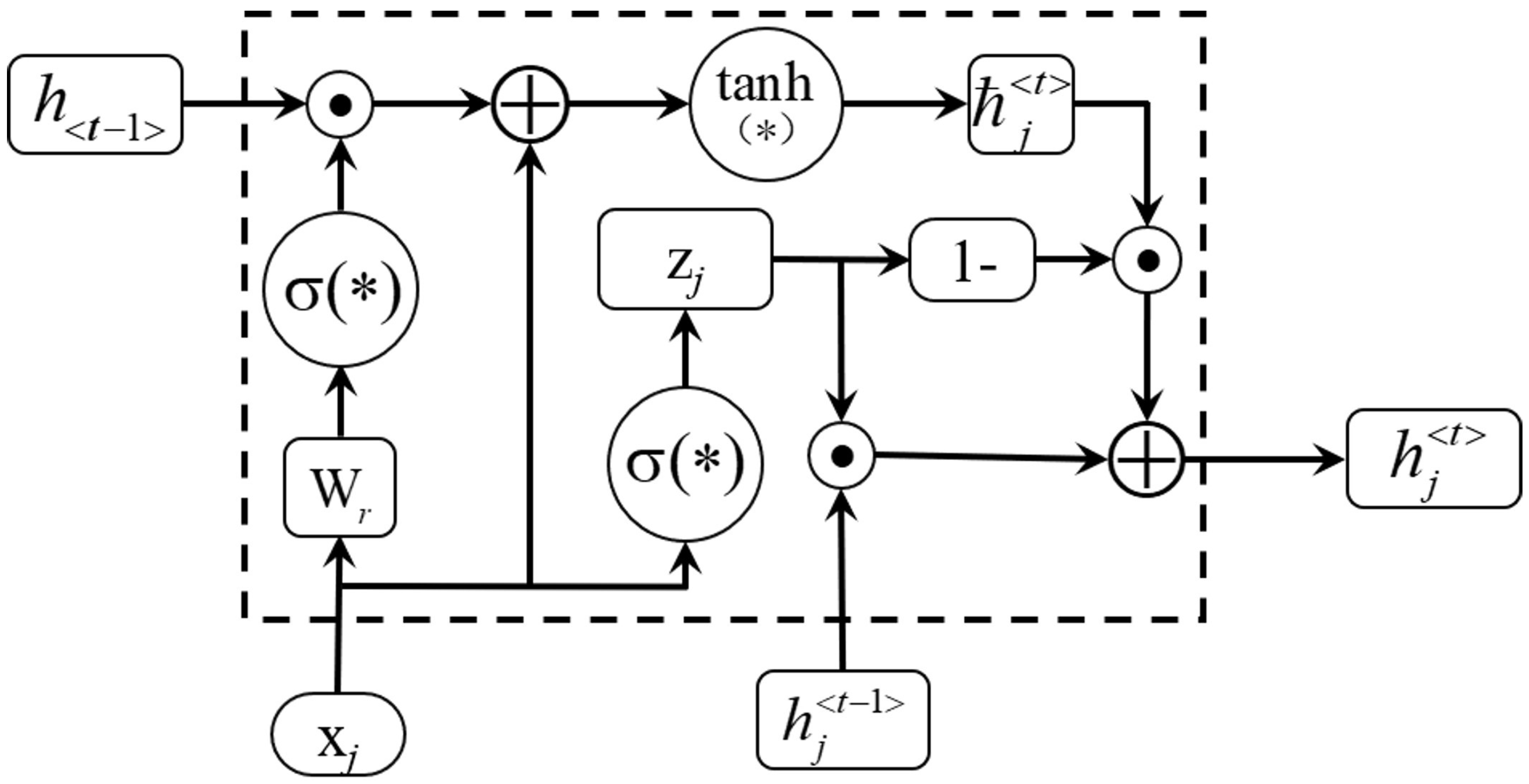
The structure of the adaptive memory and forgetting hiding unit is shown in Figure 1.

The reset gate is calculated as in Equation (1).

$$r_j=\sigma \left({\left[W_{r}x\right]}_j+{\left[U_r{h}_{<t-1>}\right]}_j\right)$$

(1)

where $\sigma$ is the logistic sigmoid activation function, $[\ast ]j$ denotes the jth element of the vector, x means input, and $h_{t-1}$ is the previous moment to pass the status. The matrices $W_r$ and $U_r$ are known weight matrices.

The update gate is calculated by Equation (2).

$$z_j=\sigma \left({\left[W_{z}x\right]}_j+{\left[U_z{h}_{<t-1>}\right]}_j\right)$$

(2)

where $h_j$ is the target cell state vector, which is calculated by Equations (3) and (4).

$${\mathit{h}}_j^{<t>}={\mathit{z}}_j\odot {\mathit{h}}_j^{<t-1>}+\left(1-{\mathit{z}}_j\right)\odot {\hslash }_j^{<t>}$$

(3)

$${{\hslash }_j}^{<t>}=\tan h\left({\left[\mathbf{Wx}\right]}_{\mathrm{j}}+{\left[\mathbf{U}\left(\mathbf{r}\odot h_{\langle t-1\rangle }\right)\right]}_j\right)$$

(4)

where ⊙ denotes element-by-element multiplication.

3.2. Two-Way Dissemination Mechanism

The disadvantage of one-way dissemination is that it cannot make use of future information and may miss some important contextual information, especially when dealing with long sequences. In addition, it is susceptible to gradient disappearance, which may lead to a decrease in the accuracy of the model.

In time series forecasting, the use of bi-directional propagation allows both past and future information to be considered, thus better capturing the past and future information of the series and improving the accuracy of the model.

Forward dissemination:

$${\mathit{r}}_t^f=\sigma \left({\left[{\mathit{W}}_r^f{\mathit{x}}^f\right]}_t+{\left[{\mathit{U}}_r^f{\mathit{h}}_{\langle t-1>}^f\right]}_t\right)$$

(5)

$${\mathit{z}}_t^f=\sigma \left({\left[{\mathit{W}}_z^f{\mathit{x}}^f\right]}_t+{\left[{\mathit{U}}_z^f{\mathit{h}}_{<t+1>}^f\right]}_t\right)$$

(6)

$${\mathit{h}}_t^f={\mathit{z}}_t^f\odot {\mathit{h}}_{t+1}^f+\left(1-{\mathit{z}}_t^f\right)\odot {\hslash }_t^f$$

(7)

$${\hslash }_t^f=\mathbf{tanh}\left({\left[{\mathrm{W}}^f{\mathrm{x}}^f\right]}_t+{\left[{\mathrm{U}}^f\left({\mathrm{r}}^f\odot {\mathit{h}}_{<t+1>}^f\right)\right]}_t\right)$$

(8)

where ${\mathit{r}}_t^f$ denotes the forward reset gate, ${\mathit{z}}_t^f$ denotes the forward update gate, ${\mathit{h}}_t{}^f$ denotes the forward hidden state, and ${\hslash }_t{}^f$ denotes the forward candidate hidden state.

$${\mathit{r}}_t^b=\sigma \left({\left[{\mathit{W}}_r^b{\mathit{x}}^b\right]}_t+{\left[{\mathit{U}}_r^b{\mathit{h}}_{\langle t-1>}^b\right]}_t\right)$$

(9)

$${\mathit{z}}_t^b=\sigma \left({\left[{\mathit{W}}_z^b{\mathit{x}}^b\right]}_t+{\left[{\mathit{U}}_z^b{\mathit{h}}_{<t+1>}^b\right]}_t\right)$$

(10)

$${\mathit{h}}_t^b={\mathit{z}}_t^b\odot {\mathit{h}}_{t+1}^b+\left(1-{\mathit{z}}_t^b\right)\odot {\hslash }_t^b$$

(11)

$${\hslash }_t^b=\mathbf{tanh}\left({\left[{\mathrm{W}}^b{\mathrm{x}}^b\right]}_t+{\left[{\mathrm{U}}^b\left({\mathrm{r}}^b\odot {\mathit{h}}_{<t+1>}^b\right)\right]}_t\right)$$

(12)

where ${\mathit{r}}_t^b$ denotes the backward reset gate, ${\mathit{z}}_t^b$ denotes the backward update gate, ${\mathit{h}}_t{}^b$ denotes the backward hidden state, and ${\hslash }_t{}^b$ denotes the backward candidate hidden state.

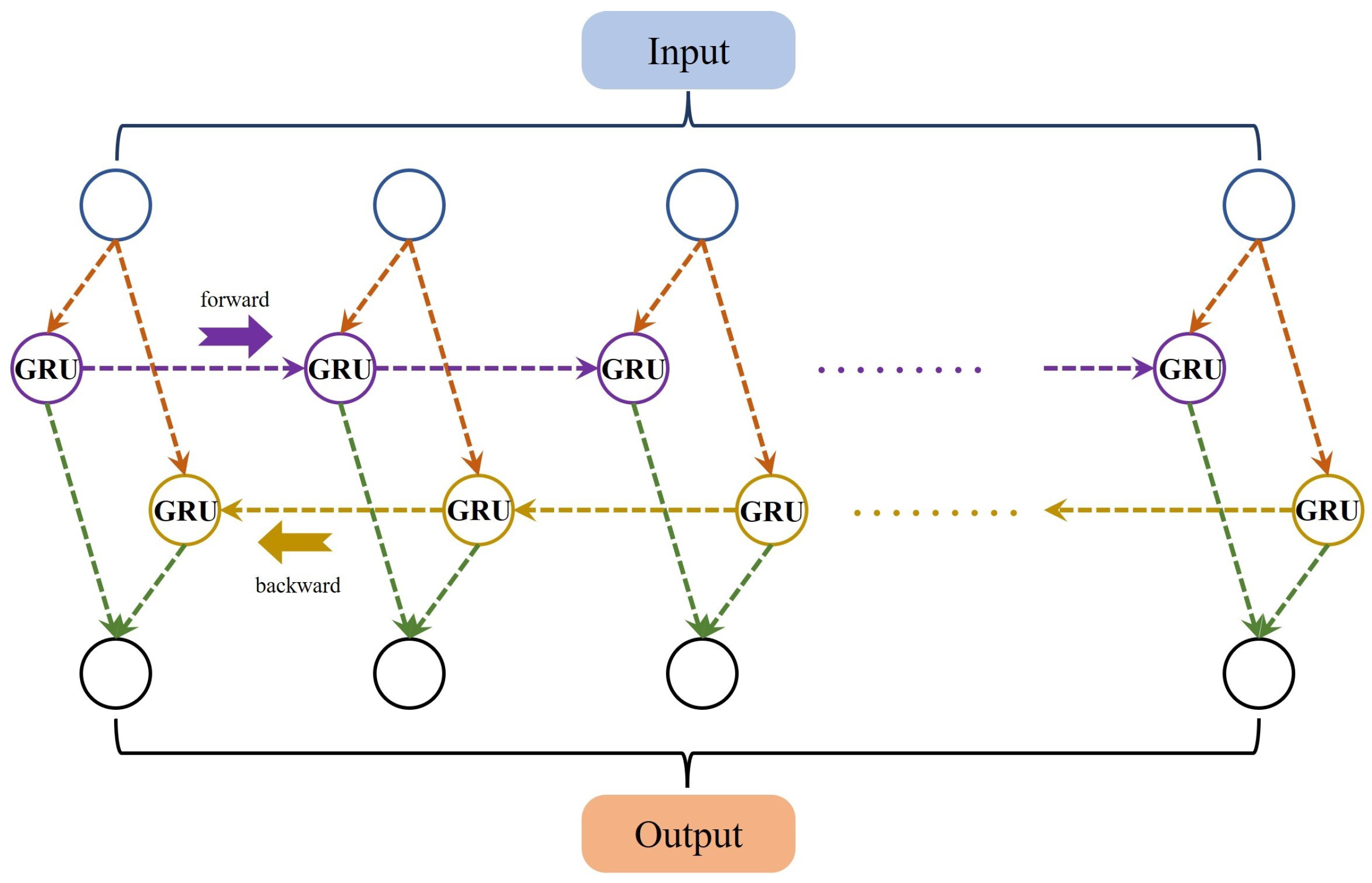
The following Figure 2 is an explanatory diagram of a BIGRU:

4. Improvements Based on ICEEMDAN and MOWOA

Neural networks work very well for data with complex relationships and non-stationary relationships, but the adaptation will be weaker than the traditional statistical method ARIMA for stationary data and simple linear relationships. Therefore, the original stock price time series data are first decomposed by ICEEMDAN, and the decomposition yields a subset of stationary and non-stationary series. The non-stationary and stationary subseries are then modeled using BIGRU and ARIMA, respectively. The whale optimization algorithm of multi-objective optimization is introduced to hyperparameterize both, which allows the model to find the parameter vector closest to the optimal solution and improves the accuracy of both models. Finally, the results of each subseries are combined to derive the final stock price prediction results.

The framework of the improved BIGRU algorithm is detailed in Figure 3.

4.1. ICEEMDAN-Based Data Decomposition and Its Class Determination

4.1.1. Decomposition of the Original Sequence

To solve the problems of CEEMDAN regarding residual noise and spurious patterns, Colominas proposed an improved CEEMDAN [9]. In contrast to CEEMDAN, which directly includes white noise in the decomposition process, ICEEMDAN selects the kth IMF component added to the white noise after it has been decomposed by EMD. The pre-processed time series data are brought into the ICEEMDAN algorithm, and the decomposition results of the sub-series can be derived. Let ${\mathrm{E}}_{\mathrm{k}}(.)$ be the kth IMF component generated by EMD, and M(.) be the operator that generates the local mean. Define $〈.〉$ to be the operator that averages the I local means. The specific decomposition steps of the CEEMDAN-based ICEEMDAN algorithm are as follows.

Step 1. The EMD is used to calculate the local mean of the Ith mixed signal $x_i\left(t\right)$, defining the first residual signal $r_1\left(t\right)$ by Equations (13) and (14).

$${\mathrm{x}}_{\mathrm{i}}\left(\mathrm{t}\right)=\mathrm{x}\left(\mathrm{t}\right)+{\epsilon }_0{\mathrm{E}}_1\left({\delta }_{\mathrm{i}}\left(\mathrm{t}\right)\right),\mathrm{i}=1,2,\dots ,\mathrm{I}$$

(13)

$${\mathrm{r}}_1=〈\mathrm{M}\left({\mathrm{x}}_{\mathrm{i}}\left(\mathrm{t}\right)\right)〉$$

(14)

The first IMF component is calculated by Equation (15).

$${\mathrm{c}}_1\left(\mathrm{t}\right)=\mathrm{x}\left(\mathrm{t}\right)-{\mathrm{r}}_1\left(\mathrm{t}\right)$$

(15)

Step 2. The second IMF component is calculated by Equations (16) and (17).

$${\mathrm{c}}_2\left(\mathrm{t}\right)={\mathrm{r}}_1\left(\mathrm{t}\right)-{\mathrm{r}}_2\left(\mathrm{t}\right)$$

(16)

$${\mathrm{r}}_2\left(\mathrm{t}\right)=〈\mathrm{M}\left({\mathrm{r}}_1\left(\mathrm{t}\right)+{\epsilon }_1{\mathrm{E}}_2\left({\delta }_{\mathrm{i}}\left(\mathrm{t}\right)\right)\right)〉$$

(17)

Step 3. The kth (k = 3, …, K) residual signal and IMF components are calculated by Equations (18) and (19).

$$r_k\left(t\right)=〈M\left(r_{k-1}\left(t\right)+{\epsilon }_{k-1}{E}_k\left({\delta }_i\left(t\right)\right)\right)〉$$

(18)

$$c_k\left(t\right)=r_{k-1}\left(t\right)-r_k\left(t\right)$$

(19)

Step 4. The iteration stops when the EMD stopping condition is satisfied, i.e., when the first decomposition residual signal $r_K\left(t\right)$ is monotonic, and the ICEEMDAN decomposition is complete.

The flowchart of the ICEEMDAN algorithm is shown in Figure 4.

4.1.2. Subsequence Determination

After decomposing the time series data, the augmented Dickey–Fuller (ADF) test is performed for each subseries. The ADF test is based on the DF test by adding a number of differential lag terms of the original series to eliminate the autocorrelation of the error terms. The core idea of the ADF test is to use the caveat autoregressive variance to control the correlation of the error terms, so it is also more applicable to complex models. In this paper, we will use the ADF unit root test to determine the stability of each modal component, and in turn to determine the model to which the modal component applies.

The regression with two lagged difference terms in the ADF test can be expressed as $\Delta y_t={\beta }_1{y}_{t-1}+{\beta }_2\Delta y_{t-1}+{\beta }_3{y}_{t-2}+{\beta }_4+{\beta }_{5}t$. The ADF test is a test of the coefficients of $y_{t-1}$ in this equation. If the coefficient is significantly non-zero, then the unit root hypothesis of $y_t$ will be denied, thus admitting the hypothesis that $y_t$ is stationary. If the ADF value is negative and large in absolute value, then the original hypothesis is rejected and the series is admitted to be stationary. If the ADF value is larger than the critical value, the hypothesis of non-stationarity and the existence of a unit root cannot be rejected and the series is admitted to be non-stationary.

The specific steps are as follows.

Step 1. The ADF value, p-test at 1% significant value, and t-test at 1% significant value of the series to be tested are first calculated.

Step 2. When the p-value is less than the significance level of 1% and the ADF value is less than the critical value corresponding to 1% in the t-test, the series is considered a stationary series.

Step 3. When the p-value is greater than the value at the significance level of 1%, then the series is determined to be non-stationary.

4.2. MOWOA-Based Multi-Objective Parameter Optimization

Since the training effects of BIGRUs and ARIMA are greatly influenced by the selection of hyperparameters and there is a combination of different hyperparameters with different model effects, the traditional grid search and single-objective optimization algorithms cannot find the optimization problems under the combination of multiple parameters. In this paper, the multi-objective optimization whale algorithm (MOWOA) is selected to adjust the parameters of the BIGRU and ARIMA algorithms to optimize the models, so that the models can be guaranteed to be optimal in time when different time series data are encountered.

The MOWOA is a multi-objective version of WOA proposed by Seyedali Mirjalili in 2016 [32] and is a heuristic optimization algorithm that simulates the hunting behavior of humpback whales. Humpback whales have special hunting and seining methods (bubble net foraging method), and three core mathematical models of WOA are given below, which are prey seining, bubble net foraging, and prey searching.

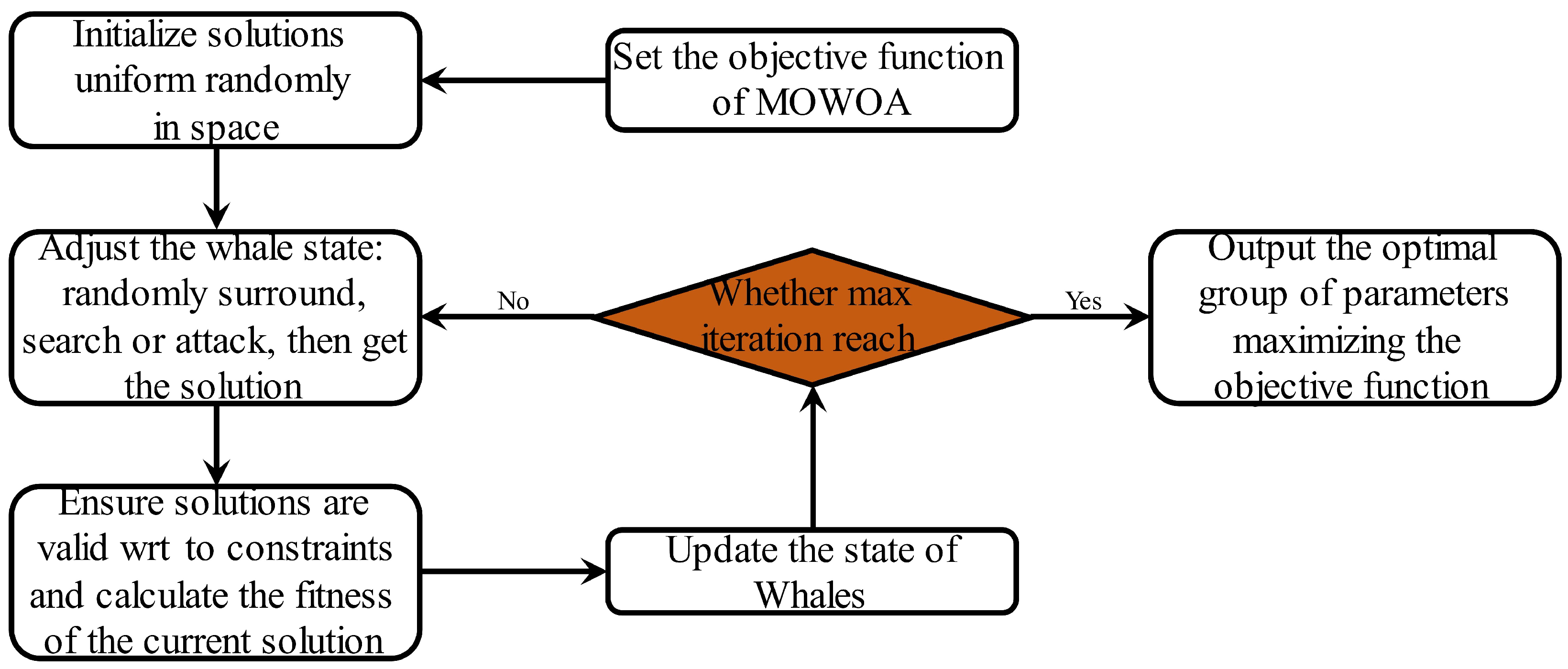
The flow chart of the MOWOA is shown in Figure 5.

4.2.1. Rounding Up Prey

The whale first searches the global solution space to determine the prey coordinates and then surrounds it. Since the optimal solution is unknown at first, the WOA assumes that the current best candidate solution is the target prey or close to the target location. After defining the best search agent, other search agents will keep converging to the best search agent, with the equations defined in Equations (20) and (21).

$$\overrightarrow{\mathrm{D}}=|\overrightarrow{\mathrm{CX}}\ast \left(t\right)-\overrightarrow{\mathrm{X}}\left(t\right)|$$

(20)

$$\overrightarrow{\mathrm{X}}(t+1)=\overrightarrow{\mathrm{X}}\ast \left(t\right)-\overrightarrow{\mathrm{A}}·\overrightarrow{\mathrm{D}}$$

(21)

where X is the current solution position vector, X* is the current optimal solution position vector, t is the current number of iterations, and A and C are the coefficient vectors.

The vectors A and C are given by Equations (22) and (23).

$$\overrightarrow{\mathrm{A}}=a\left(2r_1-1\right)$$

(22)

$$\overrightarrow{\mathrm{C}}=2\times r_2$$

(23)

The iterative process decreases linearly from two to zero. $r_1$ and $r_2$ are random vectors in [0, 1].

4.2.2. Air Bubble Net Foraging

Shrinkage bracketing mechanism: The fluctuation range of A is decreased by decreasing the value of a. Let the random vector in A be in [−a, a], then the new position of the search agent is defined as any position between the original position of the agent and the current optimal agent position.

Spiral update of position: The distance between the whale position and the prey position is first calculated, and then a spiral equation is created to mimic the humpback whale approaching the prey in a spiral pattern. The equations are shown in Equations (24) and (25).

$$\overrightarrow{\mathrm{X}}(t+1)=\overrightarrow{{\mathrm{D}}^{\prime }}·e^{\mathrm{b}l}·cos\left(2\pi l\right)+\overrightarrow{{\mathrm{X}}^{*}}\left(t\right)$$

(24)

$$\overrightarrow{{\mathrm{D}}^{\prime }}=\left|\overrightarrow{{\mathrm{X}}^{*}}\left(t\right)-\overrightarrow{\mathrm{X}}\left(t\right)\right|$$

(25)

where the whale position is (X,Y), the prey position is (X*,Y*), b is a constant defining the shape of the logarithmic spiral, and l is a random number in [−1, 1].

In order to simulate humpback whales swimming around their prey in a shrinking envelope, it was assumed that humpback whales have a 50% probability of choosing to shrink the envelope or spiral to update their position, as explained by Equation (26).

$$\overrightarrow{\mathrm{X}}(t+1)=\left\{\begin{array}{cc}\overrightarrow{\mathrm{X}}\ast \left(t\right)-\overrightarrow{\mathrm{A}}·\overrightarrow{\mathrm{D}}\hfill & \mathrm{if}p<0.5\hfill \\ \overrightarrow{{\mathrm{D}}^{\prime }}·e^{\mathrm{b}l}·cos\left(2\pi l\right)+\overrightarrow{{\mathrm{X}}^{*}}\left(t\right)\hfill & \mathrm{if}p\ge 0.5\hfill \end{array}\right.$$

(26)

where p is a random probability in [0, 1].

4.2.3. Search for Prey

The humpback whales randomly search for prey based on each other’s location, using A-vectors with random values greater than 1 in absolute value to force the search agent to be the best search agent. In the prey search phase, the humpback whales randomly select search agents to update the best search agent position. The mathematical model is shown in Equations (27) and (28).

$$\overrightarrow{\mathrm{D}}=\left|\overrightarrow{\mathrm{C}}·{\overrightarrow{\mathrm{X}}}_{\mathrm{rand}}-\overrightarrow{\mathrm{X}}\right|$$

(27)

$$\overrightarrow{\mathrm{X}}(t+1)={\overrightarrow{\mathrm{X}}}_{\mathrm{rand}}-\overrightarrow{\mathrm{A}}·\overrightarrow{\mathrm{D}}$$

(28)

where $X_{rand}$ is a randomly selected whale.

4.2.4. Multi-Objective Optimization

To solve the problem of multi-objective optimization, scientists proposed a new concept, i.e., dominates, which can find the optimal parameter vector for multi-objective functions. Without loss of generality, the optimization problem and the Pareto optimal solution are defined as follows [33,34].

Definition 1.

Optimization problem.

Optimization problems can be divided into maximization and minimization, and the two can be transformed into each other by taking the inverse operation. Therefore, the optimization problem can be written uniformly in maximization form as:

Maximize:

$$\mathrm{F}\left(\mathrm{x}\right)=f_1\left(\mathrm{x}\right),f_2\left(\mathrm{x}\right),\dots f_n\left(\mathrm{x}\right)$$

(29)

Submitted to:

$$g_i\left(\mathrm{x}\right)\ge 0,i=1,2,\dots ,j$$

(30)

$$h_i\left(\mathrm{x}\right)=0,i=1,2,\dots ,p$$

(31)

$$L_i\left(\mathrm{x}\right)\le x_i\le R_i,i=1,2,\dots ,k$$

(32)

where k is the number of variables, n is the number of objective functions, j is the number of inequality constraints, p is the number of equation constraints, $g_i$ is the i-th inequality constraint, hi denotes the i-th equation constraint, and [$L_i$, $R_i$] is the range of the i-th variable.

Definition 2.

Pareto Dominance:

The vector $\mathrm{x}=({\mathrm{x}}_1,{\mathrm{x}}_2,{\mathrm{x}}_3,...,{\mathrm{x}}_{\mathrm{i}})$ dominates the vector $\mathrm{y}=({\mathrm{y}}_1,{\mathrm{y}}_2,{\mathrm{y}}_3,...,{\mathrm{y}}_{\mathrm{i}})$ (expressed as x > y) if:

$$\forall i\in [1,k],\left[f\left(x_i\right)\ge f\left(y_i\right)\right]\wedge \left[\exists i\in [1,k]:f\left(x_i\right)\right]$$

(33)

Definition 3.

Pareto optimality:

$$\nexists y\in X\mid F\left(y\right)\succ F\left(x\right)$$

(34)

Definition 4.

Pareto optimal set:

$$P_s:=\{x,y\in \mathit{X}\mid \exists F\left(y\right)\succ F\left(x\right)\}$$

(35)

Definition 5.

Pareto optimal front:

A set including the value of objective functions for Pareto solutions set:

$${\mathit{P}}_f:=\left\{F\left(\mathit{x}\right)\mid \mathit{x}\in {\mathit{P}}_s\right\}$$

(36)

5. Experimental Simulation and Analysis of Results

5.1. Data Set Description and Processing

In this paper, four stocks in the new energy vehicle industry (Azera NIO, Ford F, Tesla Motors TSLA, and Mullen Motors MULN), which have been hot in recent years, were used as experimental data. The above data were downloaded from Yahoo Finance’s website (https://finance.yahoo.com/, accessed on 27 October 2022).

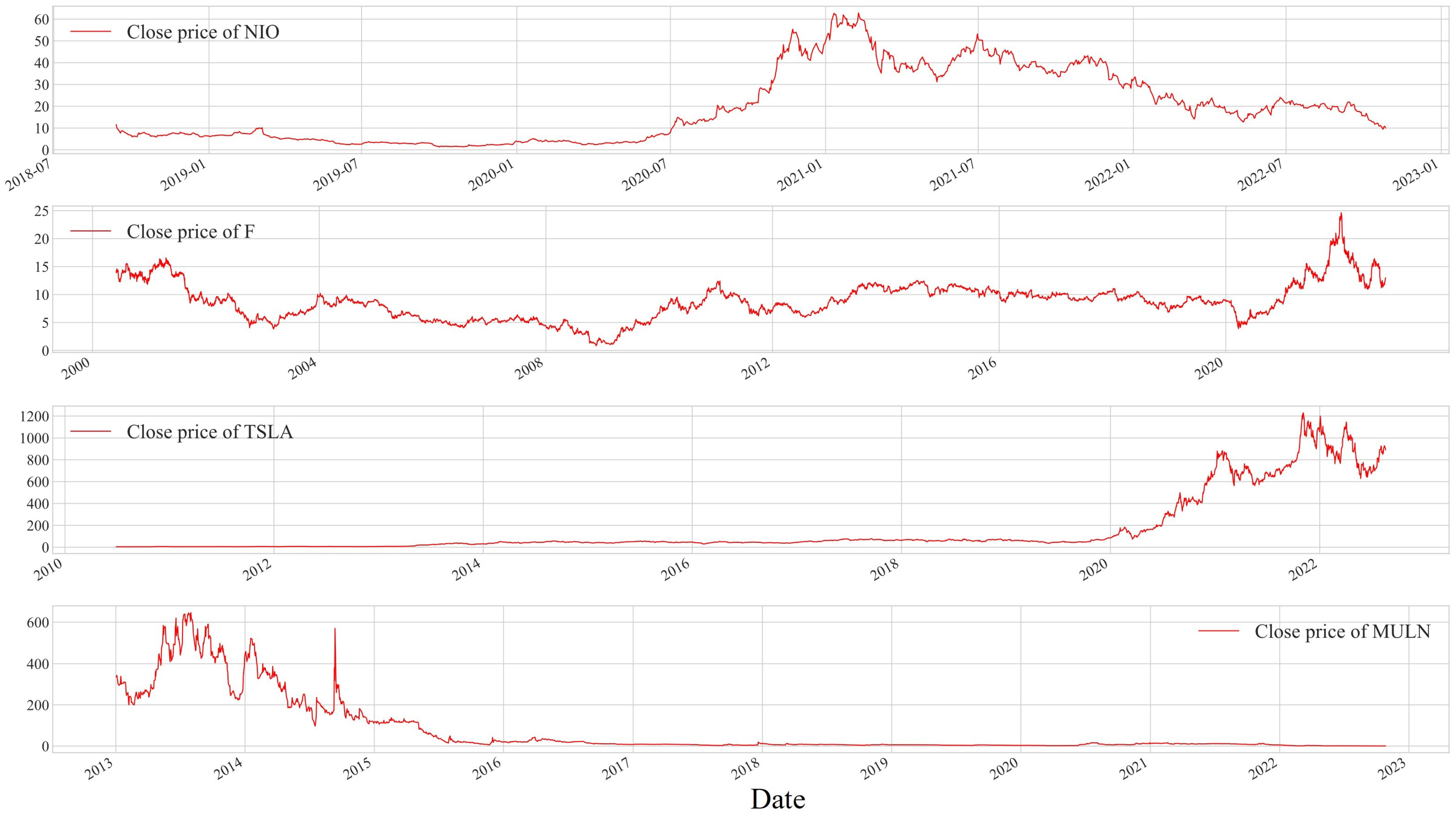
The four sets of stock data are visualized in Figure 6.

The time series curves of the four stocks in Figure 6 exhibit clear nonlinear characteristics, differing from linear or approximately linear trends. The curves display intricate patterns with twists, fluctuations, and periodic shapes, indicating complex volatility patterns. Additionally, the slopes and curvatures of the curves undergo sharp changes at different time points, showing sudden fluctuations or oscillations. These nonlinear features suggest that the data dynamics possess nonlinear characteristics, making it difficult to explain using simple linear models. This emphasizes the need for nonlinear analysis methods to better understand and interpret the behavior of these time series data. Therefore, employing a BIGRU to handle nonlinear stock price time series data aligns with the theory.

From Figure 6, it can be seen that TSLA and MULN show opposite trends, and NIO and F show overall fluctuations. The variation characteristics of the four datasets are different, and the model can be better tested in terms of generalizability.

The four sets of stock price time series data are divided into a training set and a test set as follows:

1. NIO stock price time series data: 13 September 2018 to 30 June 2021 as the training set and 1 July 2021 to 27 October 2022 as the test set.

2. F share price time series data: 1 June 2000 to 31 December 2018 as the training set and 2 January 2019 to 27 October 2022 as the test set.

3. Tesla stock price time series data: 29 June 2010 to 31 December 2020 as the training set and 4 January 2021 to 27 October 2022 as the test set.

4. MULN stock price time series data: 2 January 2013 to 31 December 2019 as the training set and 2 January 2020 to 27 October 2022 as the test set.

5.2. Evaluation Indicators

In this paper, the root mean square error (RMSE), mean square error (MSE), mean absolute error (MAE), mean absolute percentage error (MAPE), and coefficient of determination (${\mathrm{R}}^2$) are used to evaluate the predictive performance of the above models, defined by Equations (37)–(41).

$$\mathrm{RMSE}=\sqrt{\frac{{\displaystyle \sum _{\mathrm{i}=1}^{\mathrm{n}}}{({\mathrm{f}}_{\mathrm{i}}-{\mathrm{y}}_{\mathrm{i}})}^2}{\mathrm{n}}}$$

(37)

$$\mathrm{MSE}=\frac{{\displaystyle \sum _{\mathrm{i}=1}^{\mathrm{n}}}{({\mathrm{f}}_{\mathrm{i}}-{\mathrm{y}}_{\mathrm{i}})}^2}{\mathrm{n}}$$

(38)

$$\mathrm{MAE}=\frac{{\displaystyle \sum _{\mathrm{i}=1}^{\mathrm{n}}}|{\mathrm{f}}_{\mathrm{i}}-{\mathrm{y}}_{\mathrm{i}}|}{\mathrm{n}}$$

(39)

$$\mathrm{MAPE}=\frac{100\%}{\mathrm{n}}\sum _{\mathrm{i}=1}^{\mathrm{n}}\left|\frac{{\mathrm{f}}_{\mathrm{i}}-{\mathrm{y}}_{\mathrm{i}}}{{\mathrm{y}}_{\mathrm{i}}}\right|$$

(40)

$${\mathrm{R}}^2=1-\frac{{\displaystyle \sum _{\mathrm{i}=1}^{\mathrm{n}}}{({\mathrm{y}}_{\mathrm{i}}-{\mathrm{f}}_{\mathrm{i}})}^2}{{\displaystyle \sum _{\mathrm{i}=1}^{\mathrm{n}}}{({\mathrm{y}}_{\mathrm{i}}-\overline{\mathrm{y}})}^2}$$

(41)

where ${\mathrm{f}}_{\mathrm{i}}$ is the predicted value, ${\mathrm{y}}_{\mathrm{i}}$ is the actual value, and $\overline{\mathrm{y}}$ is the mean of the actual values.

5.3. ICEEMDAN Data Decomposition Results

In the ICEEMDAN decomposition of the time series data, Azera NIO was decomposed into eight IMF components, Ford F was decomposed into ten IMF components, Tesla TSLA was decomposed into ten IMF components, and Mullen MULN was decomposed into nine IMF components. The decomposition results are shown in Figure 7 below.

After decomposing the original data into multiple IMFs and RES, an ADF stationarity test was performed, and the test results are shown in

Table 1. ADF test results and determination results for each decomposition series.

Modal Components		Row Data	IMF1	IMF2	IMF3	IMF4	IMF5	IMF6	IMF7	IMF8	IMF9	IMF10	Res
NIO	p value	0.654	0	5.90 × 10${}^{-10}$	9.20 × 10${}^{-20}$	3.30 × 10${}^{-15}$	3.90 × 10${}^{-7}$	7.80 × 10${}^{-6}$	0.18	0.108	-	-	0.955
	ADF value	−1.24	−27.18	−7.03	−10.94	−9.11	−5.83	−5.22	−2.27	−2.52	-	-	−0.03
	t value	−3.43	−3.43	−3.43	−3.43	−3.43	−3.43	−3.43	−3.43	−3.43	-	-	−3.43
	Judgment	0	0	1	1	1	1	1	0	0	-	-	0
F	p value	0.101	2.01 × 10${}^{-23}$	0	0	0	1.80 × 10${}^{-26}$	3.60 × 10${}^{-17}$	4.30 × 10${}^{-13}$	1.79 × 10${}^{-5}$	0.048	0.113	0.092
	ADF value	−2.56	−12.56	−34.87	−24.68	−23.34	−14.19	−14.63	−8.28	−5.04	−2.87	−2.5	−2.6
	t value	−3.43	−3.43	−3.43	−3.43	−3.43	−3.43	−3.43	−3.43	−3.43	−3.43	−3.43	−3.43
	Judgment	0	1	1	1	1	1	1	1	1	0	0	0
TSLA	p value	0.969	3.30 × 10${}^{-18}$	1.13 × 10${}^{-19}$	0	9.09 × 10${}^{-23}$	4.42 × 10${}^{-20}$	1.61 × 10${}^{-17}$	0.002	0.014	0.0035	0.632	0.491
	ADF value	0.15	−10.3	−10.9	−19.55	−12.26	−11.07	−10.02	−3.89	−3.3	−3.74	−1.29	−1.58
	t value	−3.43	−3.43	−3.43	−3.43	−3.43	−3.43	−3.43	−3.43	−3.43	−3.43	−3.43	−3.43
	Judgment	0	1	1	1	1	1	1	1	0	1	0	0
MULN	p value	0.494	6.14 × 10${}^{-19}$	2.07 × 10${}^{-26}$	1.08 × 10${}^{-18}$	1.77 × 10${}^{-20}$	5.94 × 10${}^{-21}$	4.98 × 10${}^{-12}$	2.80 × 10${}^{-11}$	0.0001	0.662	-	0.399
	ADF value	−1.57	−10.6	−14.16	−10.5	−11.24	−11.44	−7.87	−7.57	−4.63	−1.22	-	−1.76
	t value	−3.43	−3.43	−3.43	−3.43	−3.43	−3.43	−3.43	−3.43	−3.43	−3.43	-	−3.43
	Judgment	0	1	1	1	1	1	1	1	1	0	-	0

below, which includes the calculated p values, ADF values, t values, and the judgment results. From the p-test and t-test results, the determination results can be derived (1 for series stability and 0 for instability).

5.4. MOWOA Parameter Optimization

There are many parameters that affect the performance of BIGRUs. In order to reduce the amount of operations, the three most important parameters (num_layers, hidden_size, and learning_rate) that have the greatest impact on the model effect were selected for a combination optimization in the experiment. The parameters are explained in

Table 2. BIGRU hyperparameters explained.

Parameter Name	Parameter Explanation
num_layers	Number of GRU layers in the network
hidden_size	Size of hidden layers in GRU layers
learning_rate	Learning rate

below.

5.5. Analysis and Comparison of Model Results

The original BIGRU, ICEEMDAN-optimized BIGRU, and MOWOA-optimized BIGRU were finally used for an experimental simulation comparison with the improved BIGRU in this paper. Experimental validation of the trained model was performed using a test set.

The simulation results in Figure 8 show that the improved BIGRU proposed in this paper has an excellent prediction ability for the NIO stock price time series dataset. Numerically, the improved method calculates the best value for the coefficient of determination ${\mathrm{R}}^2$ of 0.981 and it has the smallest error in all four terms. From the fitting effect, the improved method predicts values closer to the original value curve and draws a scatter plot closer to the y = x line. On the contrary, the other three algorithms have scatter plots with different degrees of shifts compared to the y = x line. Collectively, the accuracy ranking of the four algorithms for this dataset is IMPROVED METHOD > ICEEMDAN-BIGRU > MOWOA-BIGRU > BIGRU.

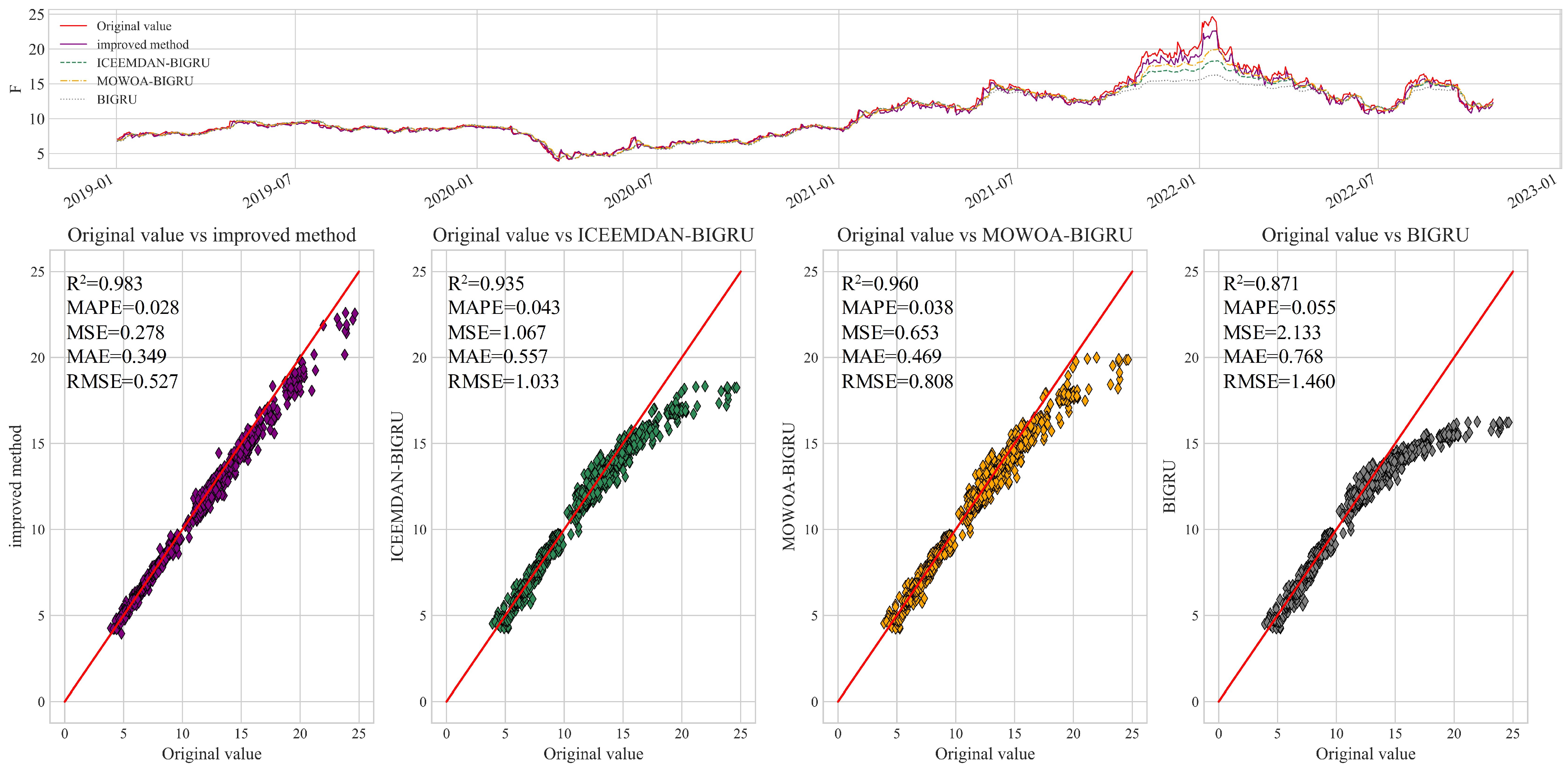
As the simulation results in Figure 9 show, the improved BIGRU proposed in this paper exhibits an excellent forecasting ability on the time series dataset of stock prices of F. Numerically, the improved method calculates the best value of the coefficient of determination ${\mathrm{R}}^2$ of 0.983 and it has the smallest error in all four terms. The method proposed in this paper obtains the lowest MAPE, MSE, MAE, and RMSE values, which shows its excellent performance in predicting the stock price of F companies. The improved method is able to capture the trends and patterns of the stock price time series data more accurately, resulting in more accurate forecasts. The scatter plot is closer to the y=x line, indicating a higher agreement between the predicted and actual values; thus, the proposed method is more reliable in predicting the stock price of F companies. Collectively, the accuracy ranking of the four algorithms for this dataset is IMPROVED METHOD > MOWOA-BIGRU > ICEEMDAN-BIGRU > BIGRU.

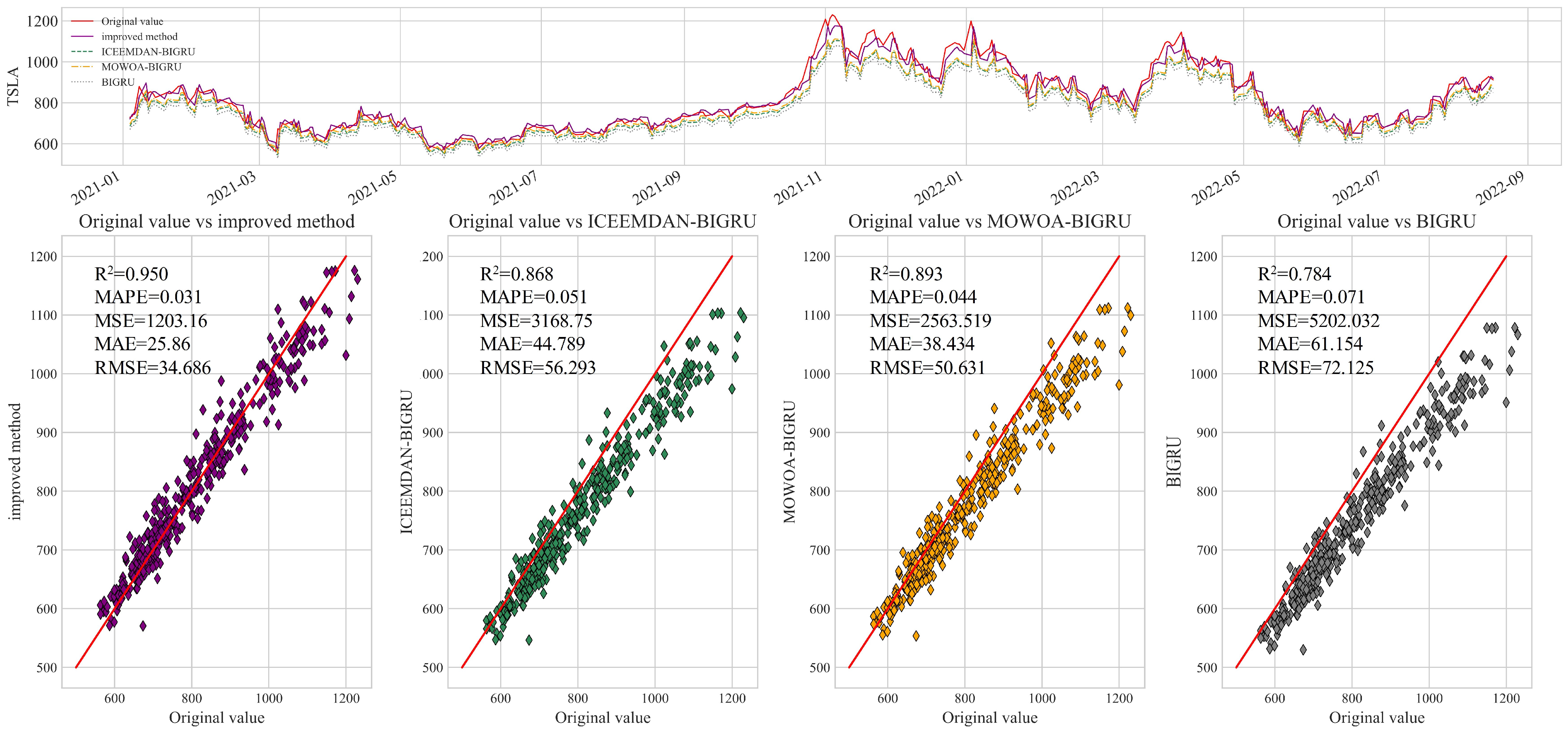
As the simulation results in Figure 10 show, the improved BIGRU proposed in this paper still exhibits an excellent prediction capability on TSLAs stock price time series dataset. Numerically, the improved BIGRU proposed in this paper computes the best coefficient of determination, with an ${\mathrm{R}}^2$ value of 0.950 on the TSLA stock price time series dataset, and it has the smallest of all four error indicators. This shows that the improved method has excellent performance in predicting the stock prices of TSLA. Through a comparative analysis, the improved method proposed in this paper has a high prediction performance on predicting the stock time series dataset of TSLA. The improved method can better utilize the correlation information in the stock price time series data to improve the prediction accuracy, which provides useful information and a reference for stock price prediction and research in related fields. Collectively, the accuracy ranking of the four algorithms for this dataset is IMPROVED METHOD > MOWOA-BIGRU > ICEEMDAN-BIGRU > BIGRU.

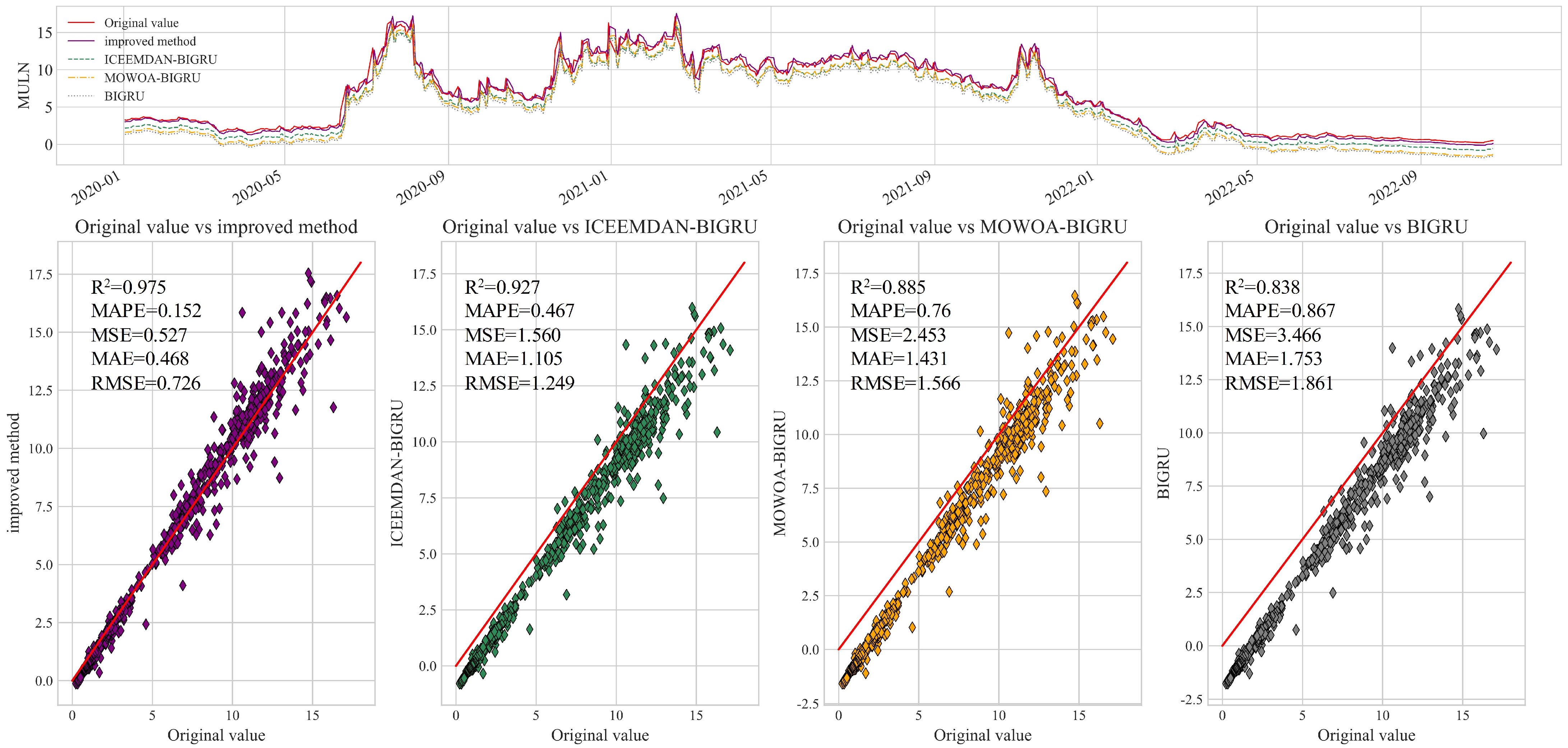
As the simulation results in Figure 11 show, the improved BIGRU proposed in this paper still exhibits an excellent prediction capability on the MULN stock price time series dataset. Numerically, the improved BIGRU proposed in this paper computes the best determination coefficient, with an ${\mathrm{R}}^2$ value of 0.975 on the MULN stock price time series dataset, and it has the smallest of the four error metrics. Through a comparative analysis, the improved method proposed in this paper has a higher prediction performance on the stock time series dataset for predicting MULN. Collectively, the accuracy ranking of the four algorithms for this dataset is IMPROVED METHOD > ICEEMDAN-BIGRU > MOWOA-BIGRU > BIGRU.

6. Discussion

Through a comparative analysis of the simulation results on the test sets of the four stock price time series data, it has been demonstrated that the proposed enhancements are capable of accurately capturing the trends and patterns within the data, thereby achieving more precise predictions.

In this study, three control group experiments were conducted, namely ICEEMDAN-optimized BIGRU, MOWOA-optimized BIGRU, and unoptimized BIGRU. Five evaluation metrics were utilized to assess the performance. An analysis of the prediction results on the four stock price datasets revealed that both ICEEMDAN and MOWOA provided noticeable improvements to the BIGRU, and combining these techniques yielded even greater enhancement in its performance.

The proposed enhancement method exhibited strong predictive performances when applied to the stock price time series data of NIO, F, TSLA, and MULN. The improved BIGRU effectively leveraged the correlated information within the data, resulting in an enhanced prediction accuracy. These findings offer valuable insights and references for stock price prediction and related research fields.

7. Conclusions

The improved algorithm proposed in this paper was simulated and tested on the stock price time series data of four automobile companies, namely Azera, Ford, Tesla, and Maren, in a Python 3.9 environment. Simulations were also compared with ICEEMDAN-BIGRU, MOWOA-BIGRU, and BIGRU, and the simulation results showed that:

• The use of the ICEEMDAN data decomposition method and the MOWOA with multi-objective optimization leads to different degrees of improvement on the prediction performance of the BIGRU. This indicates that ICEEMDAN allows the original BIGRU to make full use of the stationary information in the stock price time series data, and MOWOA can also find more suitable parameters for BIGRU training.
• Among the four sets of stock price time series data, the improved BIGRU model is able to better capture the trends and patterns of stock prices when predicting them, achieving more accurate forecasts. Compared with the other comparison methods, the improved model has a higher prediction accuracy and consistency.

The improved algorithm proposed in this paper can make full use of the stationary information in the stock price time series data and has a strong parameter search capability to better capture data trends and patterns and achieve more accurate predictions.