Article

A Laser Data Compensation Algorithm Based on Indoor Depth Map Enhancement

1
Jeely Automative Institute, Hangzhou Vocational & Technical School, Hangzhou 310018, China
2
School of Automation, Hangzhou Dianzi University, Hangzhou 310018, China
3
Electric Power Research Institute of State Grid Henan Electric Power Company, Zhengzhou 450018, China
*
Author to whom correspondence should be addressed.
Electronics 2023, 12(12), 2716; https://doi.org/10.3390/electronics12122716
Submission received: 6 May 2023 / Revised: 6 June 2023 / Accepted: 13 June 2023 / Published: 17 June 2023

Abstract

:
The field of mobile robotics has seen significant growth regarding the use of indoor laser mapping technology, but most two-dimensional Light Detection and Ranging (2D LiDAR) can only scan a plane of fixed height, and it is difficult to obtain the information of objects below the fixed height, so inaccurate environmental mapping and navigation mis-collision problems easily occur. Although three-dimensional (3D) LiDAR is also gradually applied, it is less used in indoor mapping because it is more expensive and requires a large amount of memory and computation. Therefore, a laser data compensation algorithm based on indoor depth map enhancement is proposed in this paper. Firstly, the depth map acquired by the depth camera is removed and smoothed by bilateral filters to achieve the enhancement of depth map data, and the multi-layer projection transformation is performed to reduce the dimension to compress it into pseudo-laser data. Secondly, the pseudo-laser data are used to remap the laser data according to the positional relationship between the two sensors and the obstacle. Finally, the fused laser data are added to the simultaneous localization and mapping (SLAM) front-end matching to achieve multi-level data fusion. The performance of the multi-sensor fusion before and after is compared with that of the existing fusion scheme via simulation and in kind. The experimental results show that the fusion algorithm can achieve a more comprehensive perception of environmental information and effectively improve the accuracy of map building.

1. Introduction

With the continuous application of the intelligent interaction of mobile robots in daily life, the SLAM technology of multi-sensor fusion can better obtain the redundant information of the map, improve the robustness and stability of the map, and provide a good technical foundation for the next step of localization and navigation.
Laser sensors can accurately and rapidly sense the information of the surrounding environment and enable real-time map building; the complexity of the calculation is low, laser sensor is widely used in SLAM map building [1]. Nowadays, most laser scan matching is realized iteratively between point clouds, which is too computationally intensive in the subsequent front-end matching and affects the real-time performance of the whole system. Lei et al. [2] proposed a LiDAR scanning algorithm in the polar coordinate system, which first expresses the LiDAR scanning angle and detection distance in a polar coordinate system by expressing the LiDAR distance measurement distribution in different orientations; this is achieved by putting the indoor object area in a functional form. However, this algorithm is limited to indoor map building for small scenes, and the cumulative error becomes larger as the map expands. Rui et al. [3] proposed the use of Inertial Measurement Unit (IMU) data to process the distortion of laser scans and extract feature points for inter-frame matching to enhance the scan alignment. However, the pose transformation provided by IMU can only be used to provide a priori information for laser point cloud matching, and IMU data are not added as a constraint to global map optimization in order to improve map consistency.
However, most pure laser SLAM algorithms are unable to sense objects under a certain height (1 m), leading to inaccurate map building and navigation errors. One current solution to this problem is to fuse visually transformed pseudo-laser data algorithms in order to reduce the limitation of the vertical view of LiDAR. Grinvald et al. [4] transformed the depth point cloud into pseudo-laser points and then fused the pseudo-laser points with the laser point cloud to achieve loopback detection using visual features. This solution not only increases the amount of computation, but also reduces the detection range of LiDAR. Wang et al. [5] predicted the initial pose of the robot based on the extended Kalman filter (EKF), combined the optimized pose with the depth point cloud and converted it into a pseudo-laser point cloud, and used an occupancy raster map algorithm to fuse the LiDAR map with the depth camera map. Compared with traditional methods, an additional pose estimation is required, which is not conducive to real-time map construction. Due to the disadvantages of laser data, such as clutter and data noise, Xin et al. [6] proposed a depth-map-based LiDAR point cloud densification algorithm, which uses triangular linear interpolation and random sampling consistency to transform the point cloud into an image and form the corresponding dataset, thus ensuring the accuracy of the laser data; however, the algorithm assumes a constant laser scanning height and the interpolation assumptions are somewhat idealized, so its effect in variable outdoor areas is not obvious. Zhang et al. [7] proposed a Bayesian estimation method for the secondary fusion of a map generated using a depth camera and LiDAR, and adopted a map construction algorithm based on map optimization during map construction. However, due to the excessive weight of depth camera fusion, the dominant role of LiDAR in map building can be seriously affected, resulting in large map errors.
Such 2D LiDAR can be used for real-time navigation, but 2D imaging lacks altitude information and cannot be used for imaging. Conversely, 3D LiDAR can be used for 3D dynamic real-time imaging with high precision and a long range. However, considering the cost and experimental scenarios, this paper chooses the combination of 2D LiDAR and a depth camera to achieve a higher measurement accuracy at a lower cost. To address the problems arising from multi-sensor fusion, this paper proposes an algorithm for fusing depth cameras and LiDAR. The main contributions of this paper are as follows:
(1)
The concept of pseudo-laser data is introduced, and the converted pseudo-laser data are fused to the laser data to make the laser data contain more information and improve the accuracy of mapping.
(2)
Based on the processed laser data, the data model is enhanced to provide a more accurate initial iterative value for SLAM front-end matching.

2. Problem Description of Scanning Limitations

The working principle of LiDAR mainly relies on the reflection or reception of waves to detect the target in order to obtain data about the environment in which it is located, and generally we use LiDAR with a limited sweep angle. At present, with the development of the radar industry, there are some LiDAR devices on the market whose sweep angle can reach 360° and whose laser scanning distance and accuracy reach a high level; however, these can still only obtain the plane of the height at which the radar is located, and the information below its height cannot be obtained, so that if some lower obstacles or moving objects are encountered, the process of building a map will lead to the construction of the map. This can lead to incomplete map construction, resulting in large cumulative errors in subsequent positioning and navigation, and even collisions [8], which can affect the normal working of the robot.
In the actual map-building process of the robot, the LiDAR should not be installed too low, as this leads to the radar scan possessing a blind area. Take the case shown in Figure 1 as an example; assuming that the radar center is located 1 m above the ground, and the red dotted line in the figure indicates the sweep plane of the radar, then the range below the red dotted line is the blind spot of the LiDAR, and the objects below this height cannot be sensed by the radar. For example, object A can be scanned by the radar, while object B, which is less than 1 m in height, cannot be perceived by the radar. The final map is only the laser data of object A, while the laser data of object B cannot be collected.
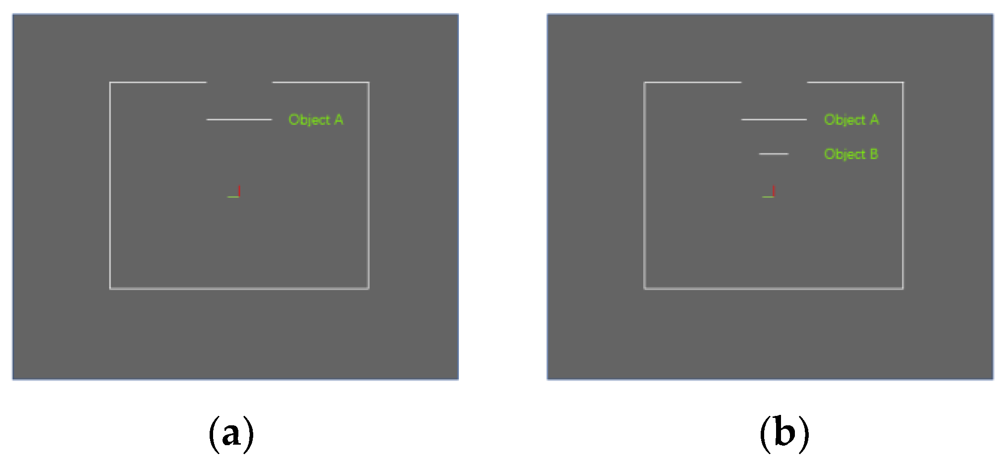
For the above scenario, the laserscan topic released by LiDAR will be significantly different compared to the actual scenario. As shown in Figure 2, the left figure is the laserscan schematic for the above scenario with incomplete scanning, while the right figure is the laserscan schematic for the real environment; it is obvious that the extra white line in the right figure is the blind area of radar scanning. The basic principle of radar map building involves using two adjacent laser data frames to match the scans and thus estimate the relative poses of the robot [9]. If the data matching of these two laser scans is used separately to perform the estimation and then update the positional and optimization process, the obtained local map will have a large offset, which will affect the construction of the global map.

3. Overview of the Fused Slam Algorithm

Combining the characteristics of depth cameras and LiDAR, we can take advantage of their mutual advantages to solve the problem of LiDAR scanning blind spots and build more complete and accurate maps. The overall process of the algorithm is as follows: firstly, dimensionality reduction is carried out on the depth value in pixel coordinates, which is converted into pseudo-laser data. Then, the image is filtered to eliminate the noise, and the laser data are associated in order to reduce data interference. Finally, the position of the obstacles is determined and the pseudo-laser data are reprojected.

3.1. Pseudo-Laser Data Conversion

To make the depth camera better fused with LiDAR, this paper uses the properties of the depth map to convert it into a form similar to the structure of laser data, i.e., pseudo-laser data [10].
In the depth camera coordinates, the downscaling of the 3D space is realized as the basis for the compensation of the laser data later. The following are the steps for the conversion of the depth maps to pseudo-laser data.
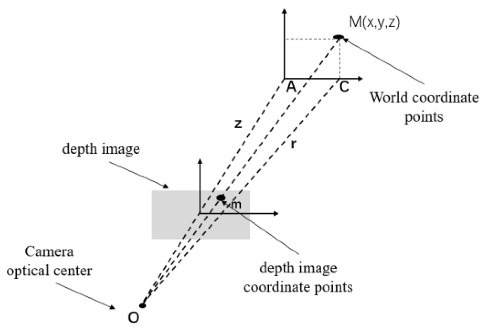
Step 1: The schematic diagram of the conversion of the depth map to pseudo-laser data is shown in Figure 3. The pixel coordinates ( u , v ) are converted to world coordinates ( X , Y , Z ) using the coordinate conversion formula, as shown in Equation (1)
[ u v 1 ] = Z c [ f x 0 u 0 0 f y v 0 0 0 1 ] [ R T ] [ X Y Z ]
In Equation (1), the pixel coordinates u and v are the number of columns and rows in its image array. The first matrix on the right is the internal reference of the camera, where f x and f y are the focal lengths of the camera in pixels, and ( u 0 , v 0 ) is the origin of the pixel coordinate system. The second matrix is the external parameter of the camera, where R and T are the rotation vector and translation vector of the camera, respectively. These internal and external parameters need to be derived by performing the calibration of the camera [11].
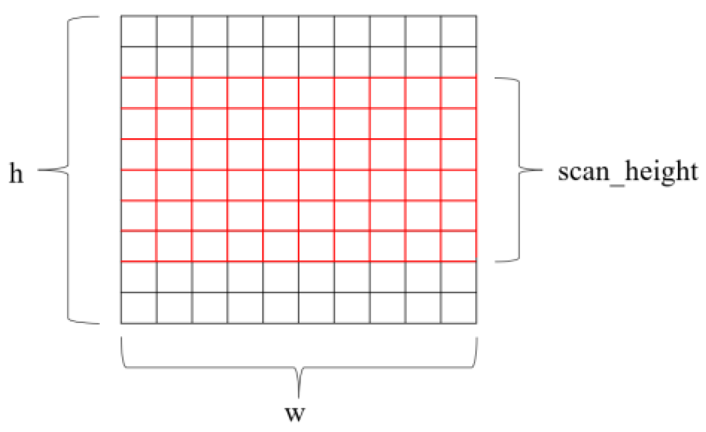
Step 2: The scan height of the depth map is obtained according to our pre-set parameter scan_height, as shown in Figure 4, and w and h represent the width and height of the pixel coordinate system, respectively.
The obstacle environmental information within the horizontal view range and the maximum vertical view height range of the depth camera are obtained and thus converted into a depth image point. First, the included angle of the obstacle point cloud θ is calculated, and the distance r, i.e., the angle between AO and CO and the distance between OC in Figure 3, is calculated as follows:
θ = atan ( x z )
r = x 2 + z 2
Step 3: The depth image is compressed using an algorithm whose basic principle is to convert the converted depth image point into pseudo-laser data by scanning it column by column in the vertical direction and forming the points of the laser signal according to the point with the smallest depth in each column, which is used as the reference. With the horizontal direction as the reference, the distance obtained in the previous step is put into the array sense[N]. It is known that the horizontal scanning angle of the depth camera is [α, β], and the angle in this range is divided into N parts; then, sense[N] can represent all the point cloud data in [α, β]. Then, the index n of the pixel in the pseudo-laser data can be expressed by Equation (4).
n = θ α β α N = N ( θ α ) ( β α )
Step 4: Therefore, the conversion between the depth map and the LiDAR data is completed via the above steps, and then these converted distances are stored in the corresponding laser data arrays. From top to bottom, all rows are scanned in turn, and if the new value is smaller, the data in the corresponding array are replaced until all rows are scanned. This completes the depth camera’s acquisition of the depth information of the object in the view and obtains the pseudo-laser data sense[k], which are prepared for the subsequent laser data fusion.

3.2. Depth Map Filtering

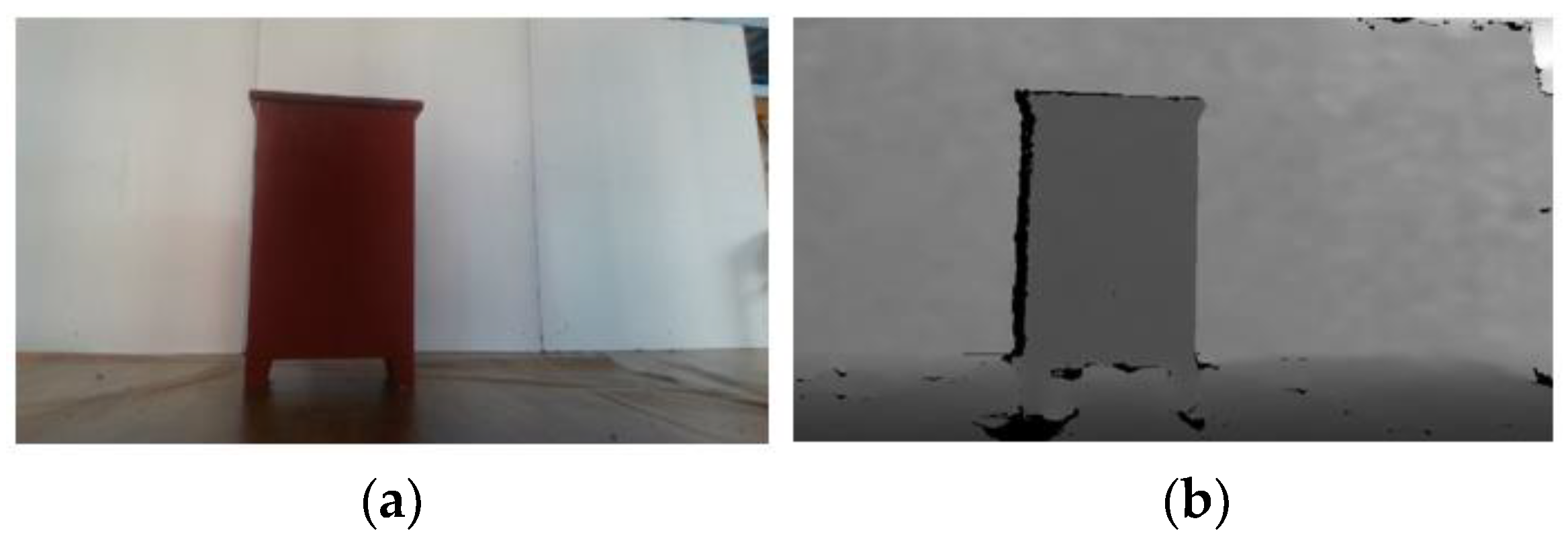
In the actual situation, due to the limitation of the principle of the depth camera and the existence of light-absorbing substances or objects with reflective properties in the environment, i.e., not so sensitive to the detection of black and transparent obstacles, and the fact that the measurement noise of the depth map is large, the depth information often has some black holes and white edges; the specific situation is shown in Figure 5, where Figure 5a,b show the depth camera for the actual laboratory, and the depth map corresponding to the color map acquired by the depth camera for the actual laboratory environment. There is a small black area and surrounding edge noise in the depth map. In the depth map, according to the gray value, a more significant black part represents the fact that the corresponding obstacle is closer to the depth camera (that is, to the robot), and a more significant white part represents the fact that the obstacle is further away from the robot.
Of course, if not through data pre-processing, then after the unprocessed depth map is converted to pseudo-laser data, the pseudo-laser data will inevitably have broken points or large data fluctuations due to too large black areas or due to too much noise in the depth image. Therefore, the depth image needs to be filtered, which can reduce the noise in the image and enhance the visual features of interest, thus making the pseudo-laser data more detailed and complete, and preparing for the next step of laser data fusion. In this paper, we use bilateral filtering to denoise the image, which is a nonlinear filter that constrains the image via the Gaussian variance of spatial distribution; it can not only complete the filtering process of the image, but also effectively protect the edge information of the image. The gray value of each pixel of the image after the bilateral filtering process is replaced by a weighted average of the gray values of the pixels in the neighborhood, and the weighting factor of the neighborhood pixels is equal to the product of the spatial-domain filter kernel function and the grayscale filter kernel function. For the pixel points to be processed, a compromise is made by combining their spatial proximity and pixel value similarity, i.e., both spatial domain information and grayscale similarity are considered. In the frequency domain analysis of the image, the edge detection needs to enhance the high-frequency band and suppress the low-frequency band; the edge information in the image is the high-frequency information, while the bilateral filtering can precisely preserve the high-frequency information and filter the low-frequency noise well to achieve the purpose of edge preservation and denoising.
d ( x , y , k , l ) = exp ( ( x k ) 2 + ( y l ) 2 2 σ d 2 )
The grayscale filtering kernel function r(x, y, k, l) is as follows:
r ( x , y , k , l ) = exp ( f ( x , y ) f ( k , l ) 2 2 σ d 2 )
The weighting factor w(x, y, k, l) is the product of d(x, y, k, l) and r(x, y, k, l):
w ( x , y , k , l ) = exp ( ( x k ) 2 + ( y l ) 2 2 σ d 2 f ( x , y ) f ( k , l ) 2 2 σ r 2 )
The specific weighting formula for the bilateral filtering is as follows:
g ( x , y ) = k , l f ( x , y ) w ( x , y , k , l ) k , l w ( x , y , k , l )
where f(x, y) is the pixel value at (x, y) in the image; g(x, y) is the pixel value at point (x, y) after the image is filtered; (k, l) is the pixel point in the neighborhood of pixel point (x, y); w(x, y, k, l) is the weight coefficient, which depends on the product of the definition domain kernel and the value domain kernel; and σ d and σ r are the standard deviation in the spatial domain and the grayscale domain, respectively.
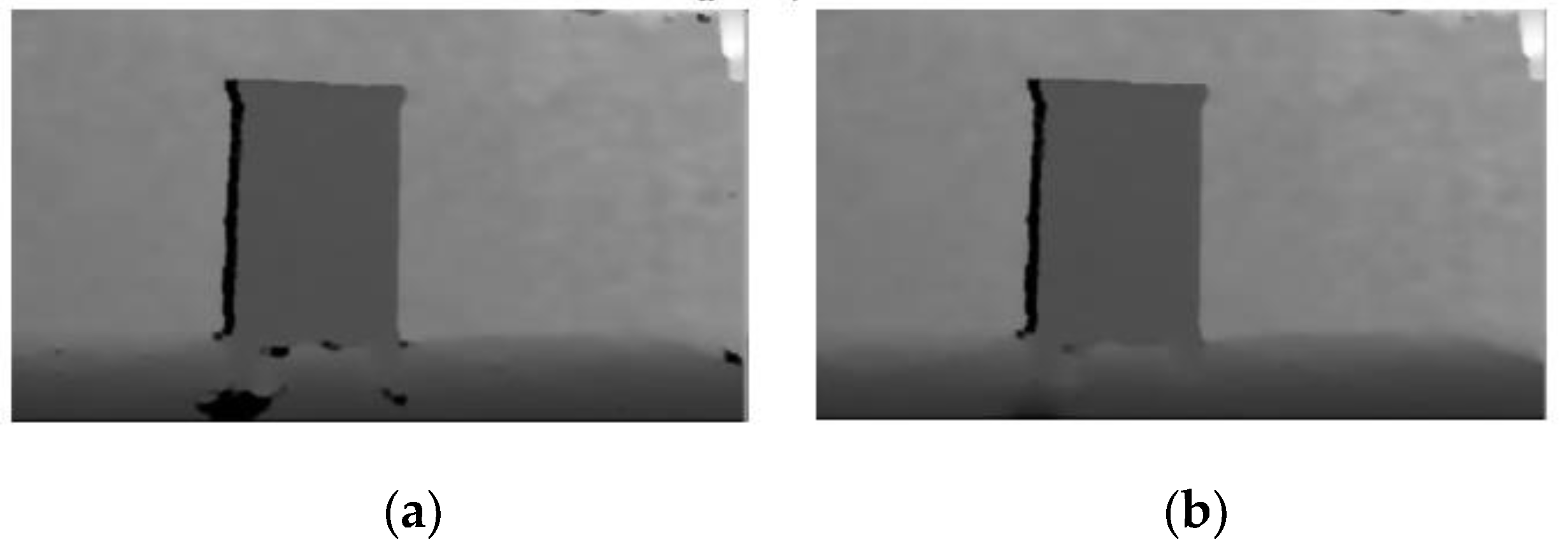
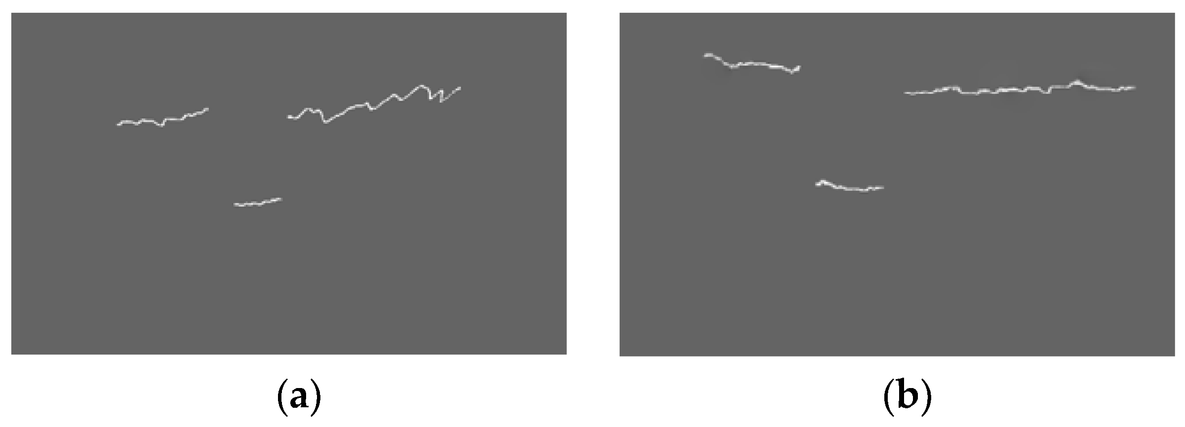
Figure 6 shows the depth comparison map before and after the bilateral filtering process, and Figure 7 shows the pseudo-laser data comparison map before and after conversion. Comparing Figure 6a with Figure 7a, the pseudo-laser data after conversion have a larger laser data fluctuation situation because the area at the bottom of the object in the figure is skeletonized, and the lower part of the whole depth map appears to be a little shadowy and noisy due to the influence of the light size. Obviously, after the image is filtered, the noise at the bottom is obviously reduced, which improves the continuity and smoothness of the transformed pseudo-laser data.

3.3. Correlation of Fused Laser Data

The laser data are not directly available for fusion, and it is necessary to determine whether they meet the data fusion conditions before fusion, i.e., to solve the data association problem of the laser data. The purpose of data correlation is to identify whether the information acquired by two sensors originates from the same object in the external environment and to reduce the interference of those data from many external environments. This is a prerequisite for multi-sensor fusion; without this step or association problems, data fusion errors and thus map-building failure would eventually occur.
Firstly, the current observed pose of the laser data can be represented by X t = ( x , y , θ ) . The data of LiDAR Z L and depth camera Z C are taken as two observations of the system, respectively, as shown in Equations (9) and (10):
Z L = H t + 1 X t + 1
Z C = H t + 1 X ^ t + 1
where H t + 1 is the observation matrix of the sensor, and the observation matrix of the depth camera and the LiDAR are the same, which is a 3 × 3 unit matrix; X t + 1 , X ^ t + 1 is the current position prediction of the sensor.
The Mahalanobis distance [12] between the observations Z L and Z C obtained by the LiDAR and the depth camera is used to determine the magnitude of the data correlation between the depth camera and the LiDAR, and when the calculated Mahalanobis Distance is less than the specified threshold γ 2 , then it can be determined that the data is highly correlated.
D i j 2 = τ t T P t + 1 1 τ t < γ 2
τ t = Z L Z C
In the above equation, τ t is the measurement error of the two sensors for the object, and P t + 1 is the covariance matrix of sensor predictions; its size is a d × d matrix, in which each element is the covariance between the different times of each sensor. When there are several features inside Z L and Z C that can be matched, it means that the features of the location data are the best match and the associated data can be fused for laser data.

3.4. Laser Data Compensation Processing

After the above processing, both the LiDAR and the depth camera obtain laser data with a horizontal viewing angle of 2 w m a x . Under normal circumstances, during the process of installing the two sensors, the vertical direction will not be on the same plumb line, that is, there is a difference in the distance between the two sensors in the horizontal direction. The laser and vision fusion scheme are shown in Figure 8. It can be seen that d i s t is the difference in the distance in the horizontal direction of the sensor, and the objects we target are those objects that cannot be detected by LiDAR, but can be detected by depth cameras. The converted pseudo-laser data and pseudo-laser data are defined as sense[k] and lidar[k], respectively, and the obstacle is determined by comparing the size relationship between them; then, a new lidar[k] is synthesized and remapped through the algorithm in this paper to form the overall laser data, and through the SLAM system, they are used for subsequent mapping and navigation functions.
The following steps are the fusion of LiDAR and the depth camera, based on the pseudo-laser data compensation algorithm.
The resolution of the depth camera used is known to be 1280 × 720, so when converting the pseudo-laser data, an array with a total index number of 1280 and elements of the pseudo-laser length are defined based on the data in the vertical direction, and then the array is traversed sequentially.
When traversing the sense[k], there are two cases before and after the critical point of k = 640 (the midpoint of 1280 pixels). That is, when k < 640, assuming that each original laser beam does not detect the obstacle, the converted pseudo-laser data can be taken and the laser data can be compensated according to the triangular transformation. It is known that ω and θ are the current detection angle of the pseudo-laser data and the angle with the sensor line, φ is the current detection angle of the synthesized laser data, and s 1 is the length of the synthesized laser data. The following equation is the formula for the process:
θ = 180 ° ± ω
s 1 = d i s t 2 + s e n s e [ k ] 2 2 d i s t · s e n s e [ k ] · c o s θ
φ = arcsin ( s e n s e [ k ] · s i n θ / s 1 )
The above equation first calculates the angle with the sensor line based on the detection angle of the pseudo-laser data at the current moment and then calculates the fused laser beam and the detection angle at this moment by combining the trigonometric constant equation. On the contrary, if k > 640, the plus and minus signs in Equation (13) are transformed.
The laser data fused in the previous step are assigned their indexes according to their scanning angles. First of all, the fused laser data from the previous step are to be compared with the original laser data in order to determine whether the laser data should be compensated. If the length of the fused laser beam is smaller than the original laser data, it means that there is an obstacle at the position of this laser data; then, the index of the data under the radar coordinate system of the laser beam again is calculated using Equation (16) according to the size of ω, and the compensated laser data are stored in the new laser data.
{ i = 180 ° φ 360 ° × N ,   ω < 0 i = 180 ° + φ 360 ° × N ,   ω > 0
where N is the total index number of the LiDAR. In addition, in those original laser beams that are larger than the fused length, indicating that there is no obstacle, the original laser data then do not need to be compensated, and the original data are stored in the array and combined with the fused data mentioned above to form the new laser data lidar[k]. The pseudo-code of the whole laser compensation algorithm is shown in Algorithm 1.
Algorithm 1 Laser Data Compensation Algorithm
Input: Pseudo-Laser Data: sense[k], Laser Data: lidar[k]
Output: Fused Laser Data: lidar[k]
while k < 1280 do
 if k < 640 then
    θ = 180 ° + ω
           s 1 = d i s t 2 + sense [ k ] 2 2 d i s t · sense [ k ] · c o s θ
    φ = arcsin ( sense [ k ] · s i n θ / s 1 )
    k = ( 180 ° φ ) / 360 ° × N
   if s 1 < lidar[k] then
   lidar[k] = s 1
 else
    θ = 18° − ω
           s 1 = d i s t 2 + sense [ k ] 2 2 d i s t · sense [ k ] · c o s θ
    φ = arcsin ( sense [ k ] · s i n θ / s 1 )
    k = ( 180 ° + φ ) / 360 ° × N
   if s 1 < lidar[k] then
   lidar[k] = s 1
 end if
end while
return lidar
After the above algorithm, the fused laser data can be finally obtained, and these compensated laser data can detect those obstacles beyond the scanning angle, and also can be used as the pre-processing of the front-end matching of SLAM to provide constraint alignment for the global map pose node estimation and realize the multi-level data fusion. At the same time, a more accurate robot state volume is output to provide the initial value of the positional pose for the next back-end optimization and closed-loop detection and to synchronize the map update [13]; the whole system overview is shown in Figure 9.

4. Simulation Analysis

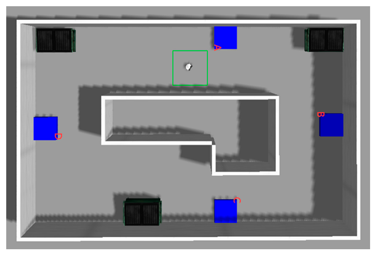
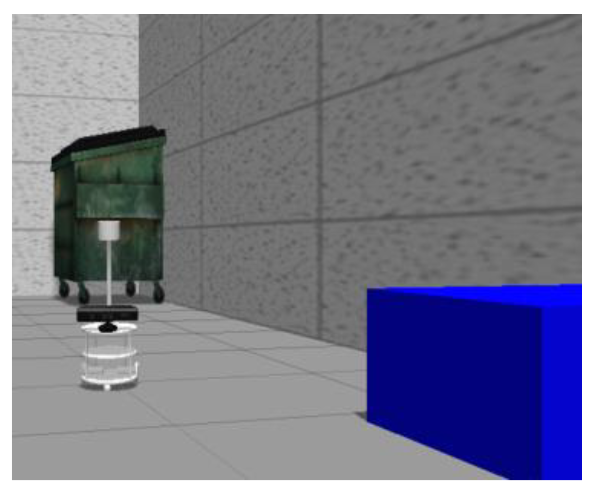
To evaluate the effect of the laser compensation algorithm designed in this paper on improving the accuracy of SLAM map building and the recognition of obstacles outside the laser view, the motion control of the robot and the construction of the active scene were performed on the gazebo system under the Robot Operating System (ROS). To recreate the actual robot-building environment, an environment was built in the gazebo system, as shown in Figure 10. In this square room, a glove box was placed on two corners and one side, and four barriers were placed on four sides. The robot model was configured according to the scale of the actual robot, as shown in Figure 11, and a depth camera was installed below the height of the LiDAR. The heights of four of the obstacles were lower than the height of the LiDAR device, and the depth camera was used to compensate for the LiDAR data on this basis.
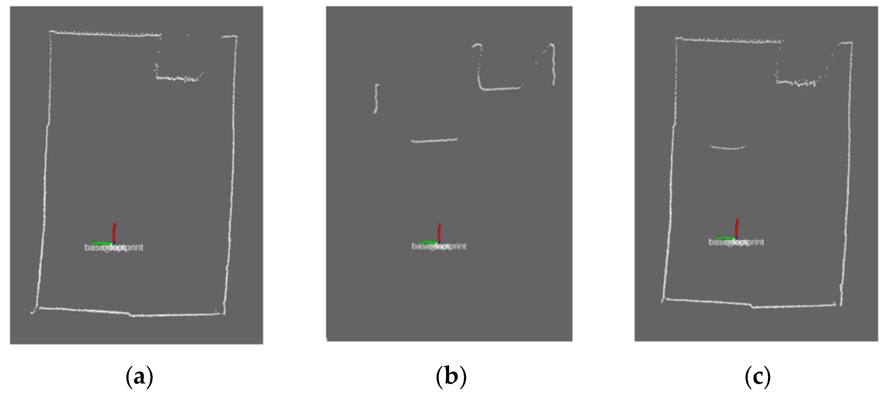
Using the robot and environment built above, the maps were constructed using the Gmapping algorithm, and the proposed scheme was verified and analyzed by analyzing the integrity of the map. The map construction results of the three solutions are shown in Figure 12, where (a) is the map using LiDAR alone, and the outline of the walls can be clearly displayed with high accuracy; however, the information on the obstacles below cannot be accurately displayed. In addition, (b) is the map generated by the pseudo-laser data and transformed by the depth camera, which is easily mismatched when the robot turns quickly, and the optimization algorithm easily falls into the local minimum; therefore, although the lower objects can be detected, misalignment occurs in the built map and the map-building effect is less satisfactory. The effect of the map built by using two sensors at the same time is shown in Figure 12c in which it can be more obviously seen that those objects that cannot be scanned by LiDAR can be shown more comprehensively. Importantly, the accuracy and precision of the created map has been greatly improved compared to that of a single sensor.
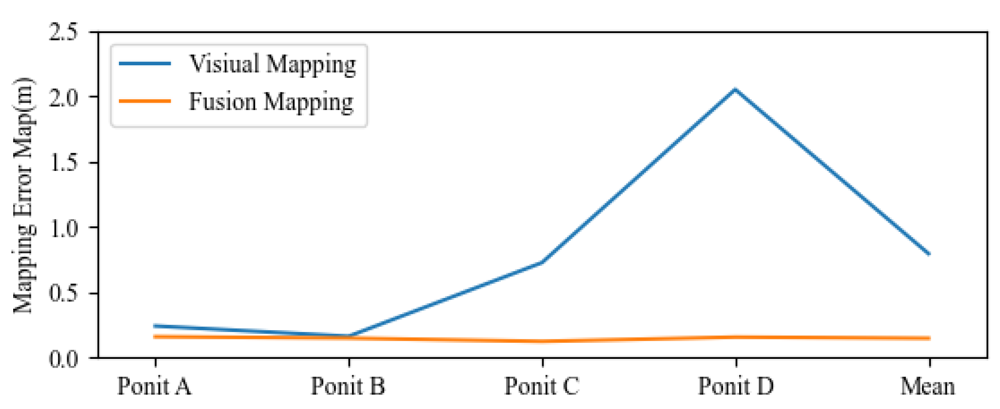
Due to the limited experimental conditions, the real value of the robot’s poses cannot be obtained, so we use the coordinate difference by comparing the actual position of the same point and the image position as a measure of the mapping effect. The simulation experiment selects the points at the four bottom edges of the four obstacles as the reference points and the starting point of the robot as the origin. It then calculates the mapping error by calculating the actual coordinates of these four points and the building coordinates, respectively. The world coordinates of the four points can be read out directly by the gazebo as the coordinate true value. In addition, the grid map coordinates after the SLAM build can be calculated via measurement. A grid on the map in rviz (a plugin in ROS) is known to correspond to 0.5 m in the real world, and it is taken as a scale to derive the map coordinates of points A, B, C, and D and calculate the respective mapping errors. The specific experimental results of the three map-building schemes are shown in Table 1 and Table 2 and Figure 13.
From the table, it can be seen that the data are not present because the map will not show the obstacle due to the laser-only build. Comparing the randomly selected coordinate points, the average error of point mapping using only the depth camera to build the map is 0.716 m, while the average error after fusing LiDAR is reduced to 0.132 m, which is 81.6% lower, indicating that the laser compensation algorithm in this paper has a great improvement effect on the accuracy of building the map.

5. Experimental Evaluation

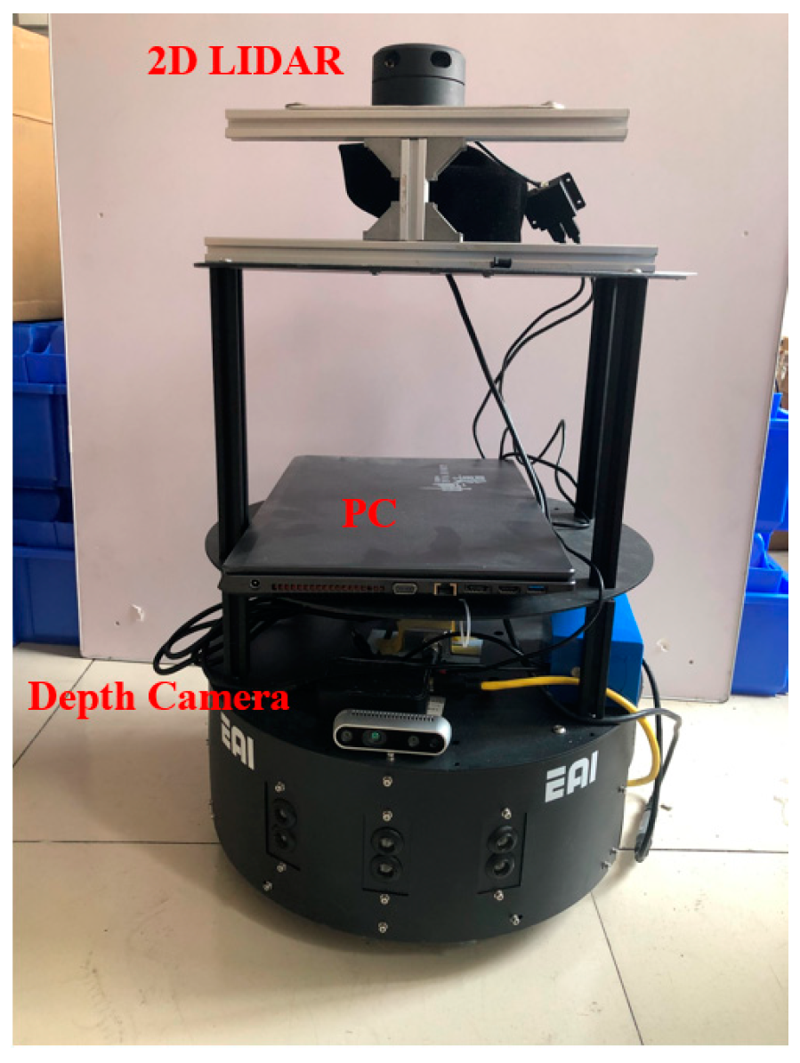
To verify the performance of the algorithm in a real-world environment, we use a two-wheel differential trolley as the robot platform. The platform is shown in Figure 14, and the robot chassis is composed of Dashgo chassis, YDLiDAR G4, and a Realsense D435i depth camera. The LiDAR is a mechanical LiDAR with a horizontal field of view of 360°, an accuracy of ±2 cm and an installation height of 0.895 m. The depth camera has a depth image resolution of 1280 × 720, a depth field of view of 86° × 57°, and a depth error of less than 2%. During the experiment, we adopt the design of the LiDAR as the main and the depth camera as the supplement to build the map, so that we can combine the advantages of both and measure the performance of fusion and building using the quantitative index. The operating system for the experiments is ubuntu 16.04, and the system runs on ROS Kinetic. The hardware configuration of the system is Intel(R) Core (TM) i7-10870H with a 2.20 GHz CPU and 8 G RAM.
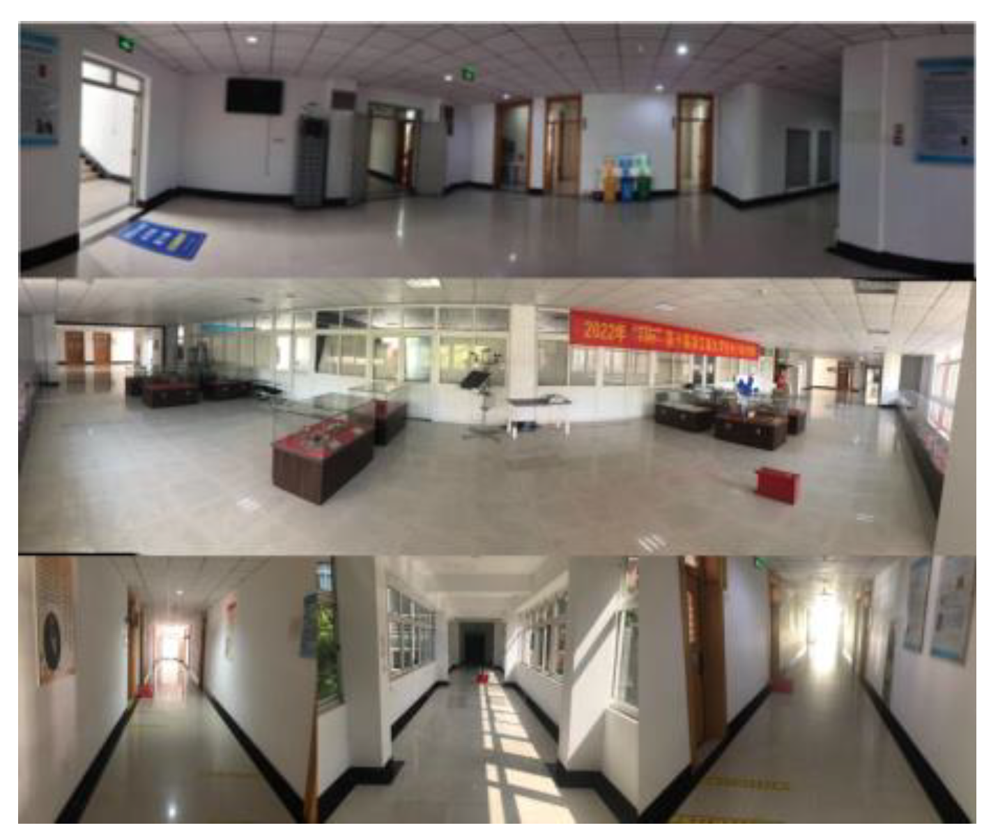
The experimental environment was set up in a rectangular corridor with a real environment that was 43 m in length and 51 m in width, covering an area of about 2193 m2, as shown in Figure 15. Structural objects such as boxes and electrical cabinets of different sizes and heights were artificially placed in the corridor, part of which was used as an obstacle for verification of the algorithm’s map-building accuracy. Because the experimental area was large and the environment was surrounded by several white wall pieces and transparent windows, the site of the experiment was chosen as a marble floor with a smooth road surface, which could effectively reduce the influence of the ground on the pseudo-laser data conversion and make the experimental data more credible.

5.1. Experiments on Fusion Laser Data

To verify the effectiveness of the fused laser data, an enclosed environment was first built and two objects were placed in front of the robot, one of which was placed below the scanning height of the LiDAR as an obstacle. The laserscan data results before and after the fusion of the LiDAR and depth camera are shown in Figure 16.
The LiDAR observation data are shown in (a), where a single LiDAR scan is more satisfactory but does not detect the obstacle at a lower position in the left front. Shown in (b) is the pseudo-laser data converted by the depth camera, where s c a n _ h e i g h t is set to 10 pixels so that the ground in the depth map has less influence on the converted laser data. It can be seen that although the converted scan angle is not large and there is noise in the rear, the outline of the obstacle below can be clearly shown. In addition, (c) represents the effect of laser data after multi-sensor fusion. The LiDAR compensates for using the data converted by the depth camera and the sensors complement each other, which can not only make up for the lack of data in the vertical direction of the LiDAR, but also maintain the range advantage of scanning in the horizontal direction.
To demonstrate the superiority of the laser compensation algorithm, 10 laser scan points are acquired at equal angles in each frame of the fused laser data, denoted by L = { ( θ 1 , d 1 ) , ( θ 2 , d 2 ) , , ( θ 10 , d 10 ) } , where ( θ n , d n ) denotes the angle and distance of the nth laser scan point in the polar coordinate system and where θ n = θ n 1 + 36 ° , θ 1 = 0 ° . The lengths of the 10 laser beams before and after fusion are counted, and their mean absolute error (MAE) and root mean square error (RMSE) are calculated, and the results are shown in Table 3.
Combined with the above table, it can be seen that for one frame of laser data sampled at equal angles, the laser has a relatively large error at 180° when using only LiDAR scanning, because it cannot scan to lower obstacles. With the advantage of the depth camera, the fused laser data significantly improve, and when combined with the laser compensation algorithm used in this paper, their accuracy significantly improves; here, the average absolute error is reduced by 65.3% and the root mean square error is reduced by 84.3%.

5.2. Experiments on Fusion SLAM Mapping

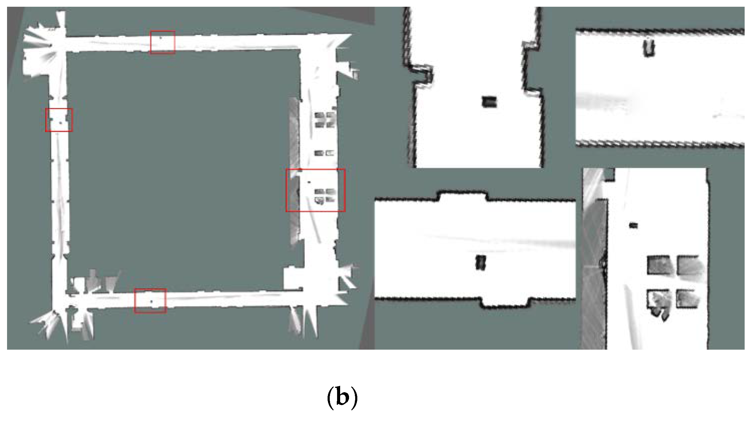
After verifying the feasibility of the depth camera to compensate for the laser data, we then verify their performance in terms of map building. Using the robot and environment in Figure 14 and Figure 15, the Cartographer algorithm (a Google open source 2D and 3D SLAM system) is used to build the map, and the proposed scheme is verified and analyzed by the completeness and accuracy of the built map. An obstacle (about 0.328 m high) is placed in each of the four corridors of the ring, in which the robot makes a circle in order to construct the environment. Figure 17 shows the SLAM map of the robot in the experimental environment, where (a) is the map constructed using LiDAR and (b) is the map after sensor fusion.
However, the experiments were performed in a corridor with similar textures, and for such a “degraded environment”, the scene restoration degree γ from the paper [14] was introduced as the experimental performance index. This can intuitively reflect the accuracy of map construction, and the formula is as follows:
γ = l m l t × 100 %
where l m is the measured value of the local structure of the SLAM mapping and l t is the length of the actual scene structure, so γ can reflect the degree to which the SLAM algorithm is restored to the real scene. From the starting point of the robot, the corridors are marked clockwise in turn as 1 to 4, and their reductions are γ 1 ~ γ 4 ; the specific values of these four parts are counted, as shown in Table 4.
Due to the limitation of the pure visual scanning angle, the observed data present obvious similarities [15]; therefore, the point cloud alignment results converge to the wrong bit pose, which seriously affects the SLAM map building effect. As such, the pure visual map building cannot be materialized. From the comparison of Figure 17 and Table 4, the reduction degree of these four parts increases by 4.11%, 0.72%, 0.26% and 0.51%, respectively, compared with that before fusion. It can be seen that the cumulative error of the single-sensor mileage in Figure 17a is large, and although it has four high reductions with consistent SLAM parameters, the γ 1 reduction sees a significant reduction, i.e., the lower-left corner has a loopback ghosting. In addition, in Figure 17b, due to the introduction of the depth camera, the vast majority of the restoration degree is improved compared with that before compensation, the loopback detection is especially obvious, the outline of obstacles can be accurately scanned, and the probability unknown area in the map is significantly reduced.
The robot’s ground truth measured with difficulty in the map building under the SLAM algorithm due to the limitation of the experimental equipment, so the computational constraint function is added to the cartographer algorithm to evaluate the cartographer’s map building by calculating the constraint-matching score ratio under different sensors and by counting the maximum, minimum and average values in the map-building process. The effect of the cartographer is evaluated by calculating the maximum, minimum and average values of the graph-building process. Usually, the cartographer algorithm builds scan matchers during construction, calculating specific constraints between nodes and subgraphs. Each submap builds a scan matcher that adds a high and low-resolution map of the active subgraph, as well as nodes within the subgraph, which are then used to match up with subsequent items to calculate the score. The higher the constraint matching score ratio is, the better the cartographer’s effect is, and its value is in the range of (0, 1). To verify the superiority of the method proposed in this paper, different sensors were compared with each other and with the current status of existing research; the study presented in [16] used a multi-sensor pose fusion method based on pose increment, and that presented in [17] used the Deutsches Museum dataset to validate the improved correlation scan matching algorithm. Since all the data could not be collected, the data with count = 8 were taken and processed as the evaluation index, and Table 5 shows the build constraint matching scores of different sensors.
As can be seen from the table, in the case of studies containing only one sensor, they possess a low matching score ratio because of the unsatisfactory pose-matching effect without the introduction of other constraints. In addition, in the research presented in [16], by adding a module that releases local pose optimization, the maximum matching ratio is significantly improved and more accurate pose estimation is obtained. Furthermore, in this paper, by fusing the two sensors, the depth camera assists in correcting the laser data, and the minimum matching score between the submaps is more accurate than the fused one. The minimum matching fraction is 9.9% higher than that of the fusion. The minimum matching score is 9.9% higher than that before fusion, and 6.8% and 14.3% higher than that in references [16], respectively; in addition, the average matching score is 5.5% higher than that before fusion. The average matching score was improved by 5.1% compared with that before fusion, and improved by 3.4% and 13.7% compared with the methods of [16], respectively. Thus, the average quality of the constructed maps was significantly improved.

6. Conclusions

A SLAM compensation algorithm based on pseudo-laser data fusion is proposed in this paper in order to address the problems of the SLAM algorithm in sensing the external environment, including the existence of blind areas in the field of view of LiDAR scanning and the occurrence of collisions in navigation. This algorithm introduces the concept of pseudo-laser data and performs data-level fusion according to the position relationship of the original laser data, so as to obtain the blind area of the field of view of the laser radar, strengthen the integrity of the observation data and improve the mapping accuracy of the SLAM algorithm. In the mapping experiment, the scene restoration degree is increased by 1.40% and the average matching score is increased by 5.1% compared with that before improvement. The experimental data show that the fusion algorithm proposed in this paper has a more comprehensive perception of the external environment and stronger robustness. It also has a more important role in improving the navigation accuracy of the robot.
On the one hand, future work should plan and generate the correct path for the navigation of the robot in an environment using dynamic obstacles [18]. On the other hand, a new loopback detection mechanism should be introduced into the laser SLAM algorithm to improve the loopback performance [19].

Author Contributions

Conceptualization, X.C., Q.W. and Q.M.; methodology, Q.M.; software, P.Z.; validation, Q.W., Q.M. and P.Z.; formal analysis, Q.M.; investigation, Q.M.; resources, Q.W.; data curation, X.C. and B.Z.; writing—original draft preparation, X.C. and Q.M.; writing—review and editing, H.L.; visualization, C.Z.; supervision, H.L.; project administration, Q.W. funding acquisition, Y.T. All authors have read and agreed to the published version of the manuscript.

Funding

This work was supported by Science and Technology Project of the State Grid Corporation of China “Research and application of visual and auditory active perception and collaborative cognition technology for smart grid operation and maintenance scenarios” (No. 5600-202046347A-0-0-00), the Fundamental Research Funds for the Provincial Universities of Zhejiang (No. GK229909299001-004).

Data Availability Statement

Data will be made available upon request from the authors.

Conflicts of Interest

The authors declare no conflict of interest.

References

  1. De Winter, A.; Baldi, S. Real-Life implementation of a GPS-Based path-following system for an autonomous vehicle. Sensors 2018, 18, 3940. [Google Scholar] [CrossRef] [PubMed] [Green Version]
  2. Lei, D.; Liu, H. A SLAM method based on LiDAR scan matching in the polar coordinates. J. Chin. Acad. Elec. Res. Inst. 2019, 14, 563–567. [Google Scholar] [CrossRef]
  3. Rui, H.; Yi, Z. High Adaptive LiDAR Simultaneous Localization and Mapping. J. Univ. Electron. Sci. Technol. China 2021, 50, 52–58. [Google Scholar] [CrossRef]
  4. Grinvald, M.; Furrer, F.; Novkovic, T.; Chung, J.J.; Cadena, C.; Siegwart, R.; Nieto, J. Volumetric Instance -Aware Semantic Mapping and 3D Object Discovery. IEEE Robot. Autom. Lett. 2019, 4, 3037–3044. [Google Scholar] [CrossRef] [Green Version]
  5. Wang, D.; Zhang, M.; Li, G. Research on SLAM of Unmanned Platform Based on the Fusion of Lidar and Depth Camera, 3rd ed.; WSAI: Sydney, NSW, Australia, 2021. [Google Scholar] [CrossRef]
  6. Xin, L.I.; Xunyu, Z.; Xiafu, P.; Zhaohui, G.; Xungao, Z. Fast ICP-SLAM Method Based on Multi-resolution Search and Multi-density Point Cloud Matching. Robot 2020, 42, 583–594. [Google Scholar] [CrossRef]
  7. Zhang, Q.Y.; Zhao, X.H.; Liu, L.; Dai, T.D. Adaptive sliding mode neural network control and flexible vibration suppression of a flexible spatial parallel robot. Electronics 2021, 10, 212. [Google Scholar] [CrossRef]
  8. Luo, C.; Wei, H.; Lu, B. Research and implementation of SLAM algorithm based on deep vision. Comput. Eng. Des. 2017, 34, 1062–1066. [Google Scholar] [CrossRef]
  9. Xue, H.; Fu, H.; Dai, B. IMU-aided high-frequency LiDAR odometry for autonomous driving. Appl. Sci. 2019, 9, 1506. [Google Scholar] [CrossRef] [Green Version]
  10. Shao, W.; Tian, G.; Zhang, Y. A 2D Mapping Method Based on Virtual Laser Scans for Indoor Robots. Int. J. Autom. Comput. 2021, 18, 747–765. [Google Scholar] [CrossRef]
  11. Zhang, Z. A flexible new technique for camera calibration. IEEE Trans. Pattern Anal. Mach. Intell. 2000, 22, 1330–1334. [Google Scholar] [CrossRef] [Green Version]
  12. Zhang, M.; Xu, X.; Chen, Y. A lightweight and accurate localization algorithm using multiple inertial measurement units. IEEE Robot. Autom. Lett. 2020, 5, 1508–1515. [Google Scholar] [CrossRef] [Green Version]
  13. Yokozuka, M.; Koide, K.; Oishi1, S.; Banno, A. LiTAMIN2: Ultra Light LiDAR-based SLAM using Geometric Approximation applied with KL-Divergence. In Proceedings of the 2021 IEEE International Conference on Robotics and Automation, Xi’an, China, 19–22 November 2021; pp. 11619–11625. [Google Scholar] [CrossRef]
  14. Xu, Y.; Yan, W.; Wu, W. Improvement of LiDAR SLAM front—End algorithm based on local map in similar scenes. Robotics 2022, 44, 176–185. [Google Scholar] [CrossRef]
  15. Liu, R.; Zhang, G.; Wang, J.; Zhao, S. Cross-modal 360° depth completion and reconstruction for large-scale indoor environment. Intell. Transp. Syst. 2022, 23, 25180–25190. [Google Scholar] [CrossRef]
  16. Zhang, L.; Liu, Z.; Cao, J.; Shen, P.; Jiang, D.; Me, L.; Zhu, G.; Qi, M. Cartographer algorithm and system implementation based on enhanced pose fusion of sweeping robot. J. Softw. 2020, 31, 2678–2690. [Google Scholar] [CrossRef]
  17. Hu, A.; Yu, G.; Wang, Q. Efficient Hardware Accelerator design of non-Linear optimization correlative scan matching algorithm in 2D LiDAR SLAM for mobile robots. Sensors 2022, 22, 8947. [Google Scholar] [CrossRef]
  18. Yin, J.; Li, A.; Li, T.; Yu, W.; Zou, D. M2dgr: A multi-sensor and multi-scenario slam dataset for ground robots. IEEE Robot. Autom. Lett. 2021, 7, 2266–2273. [Google Scholar] [CrossRef]
  19. Wei, X.; Lv, J.; Sun, J.; Pu, S. Ground-SLAM: Ground Constrained LiDAR SLAM for Structured Multi-Floor Environments. arXiv 2021, arXiv:2103.03713. [Google Scholar]
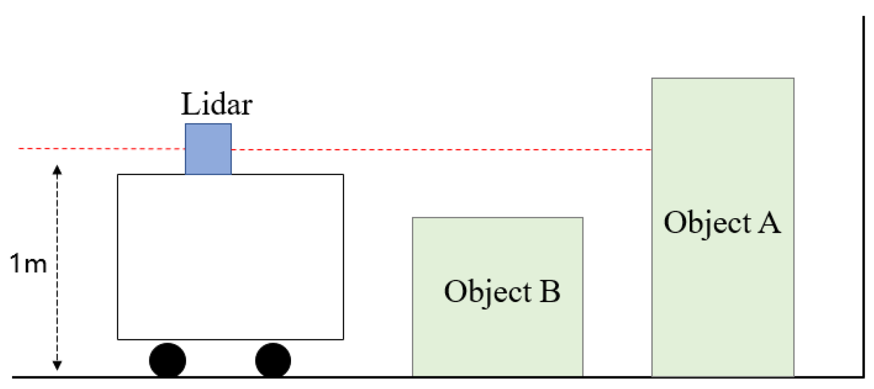
Figure 1. Schematic diagram of LiDAR scanning blind.
Electronics 12 02716 g001
Figure 2. Schematic diagram of laserscan data: (a) schematic diagram of laserscan for actual scanning; (b) schematic diagram of laserscan for the real environment.
Electronics 12 02716 g002
Figure 3. Principle diagram of pseudo-laser data conversion.
Electronics 12 02716 g003
Figure 4. Schematic diagram of depth map scanning height.
Electronics 12 02716 g004
Figure 5. Depth camera for RBD images and depth images: (a) RBD image of depth camera; (b) depth image of depth camera.
Electronics 12 02716 g005
Figure 6. Depth map before and after filtering; (a) depth map before filtering; (b) depth map after filtering.
Electronics 12 02716 g006
Figure 7. The pseudo-laser data comparison after conversion: (a) pseudo-laser data without filtered conversion; (b) pseudo-laser data after filtering and conversion (the laser data are much smoother).
Electronics 12 02716 g007
Figure 8. Schematic diagram of laser and vision fusion.
Electronics 12 02716 g008
Figure 9. System overview of SLAM algorithm for depth camera–LiDAR fusion.
Electronics 12 02716 g009
Figure 10. Simulation environment (the obstacle is one third as high and one half as wide as the box).
Electronics 12 02716 g010
Figure 11. Robot model diagram.
Electronics 12 02716 g011
Figure 12. The SLAM grid maps of the three schemes: (a) laser mapping; (b) visual mapping; (c) fusion mapping.
Electronics 12 02716 g012
Figure 13. Gmapping fusion before and after mapping error comparison line graph (laser mapping has no data).
Electronics 12 02716 g013
Figure 14. Experimental platform.
Electronics 12 02716 g014
Figure 15. Experimental environment.
Electronics 12 02716 g015
Figure 16. Laser data diagram of the three schemes: (a) laser data; (b) pseudo-laser data; (c) fusion laser data.
Electronics 12 02716 g016
Figure 17. Comparison of SLAM before and after fusion: (a) the map before fusion; (b) the map after fusion (the red area shows the obstacle).
Electronics 12 02716 g017aElectronics 12 02716 g017b
Table 1. Visual mapping error comparison.
Real CoordinatesMeasured CoordinatesError/m
A(1.045, 0.746)(1.271, 0.830)0.241
B(5.755, −2.133)(5.891, −2.079)0.146
C(2.048, −5.954)(2.688, −6.247)0.704
D(−5.914, −3.256)(−4.153, −3.450)1.772
Mean0.716 m
Table 2. Fusion mapping error comparison.
Real CoordinatesMeasured CoordinatesError/m
A(1.045, 0.746)(1.182, 0.765)0.138
B(5.755, −2.133)(5.899, −2.129)0.134
C(2.048, −5.954)(2.160, −5.968)0.113
D(−5.914, −3.256)(−5.774, −3.290)0.144
Mean0.132 m
Table 3. Comparison table of distance error before and after laser data compensation.
Actual Distance/mDistance before Fusion/mError/mDistance after Fusion/mError/m
0.7200.684−0.0360.682−0.028
36°0.7810.8040.0230.8050.024
72°0.8380.789−0.0490.791−0.047
108°0.7760.715−0.0610.718−0.058
144°1.1351.086−0.0491.081−0.054
180°1.0132.0621.0490.932−0.081
216°2.0411.997−0.0441.979−0.062
252°1.3031.256−0.0471.252−0.051
288°1.2341.188−0.0461.183−0.051
324°0.8620.9100.0480.9070.045
MAE/m0.14420.0501
RMSE/m0.33450.0524
Table 4. Comparison of restoration degree of different algorithms.
Cartographer AlgorithmCartographer Compensation Algorithm
γ 1 93.57%97.68%
γ 2 95.56%96.28%
γ 3 97.06%97.32%
γ 4 96.78%97.29%
Table 5. Matching score ratio of each sensor combination and the literature.
MinMaxMean
Lidar0.6200.7910.712
Camera0.6360.7990.690
Paper [16]0.6510.8240.729
Paper [17]0.6290.7750.671
Lidar + Camera0.7190.8020.763
Disclaimer/Publisher’s Note: The statements, opinions and data contained in all publications are solely those of the individual author(s) and contributor(s) and not of MDPI and/or the editor(s). MDPI and/or the editor(s) disclaim responsibility for any injury to people or property resulting from any ideas, methods, instructions or products referred to in the content.