Optimizing Neural Networks for Imbalanced Data

Abstract

Imbalanced datasets pose pervasive challenges in numerous machine learning (ML) applications, notably in areas such as fraud detection, where fraudulent cases are vastly outnumbered by legitimate transactions. Conventional ML methods often grapple with such imbalances, resulting in models with suboptimal performance concerning the minority class. This study undertakes a thorough examination of strategies for optimizing supervised learning algorithms when confronted with imbalanced datasets, emphasizing resampling techniques. Initially, we explore multiple methodologies, encompassing Gaussian Naive Bayes, linear and quadratic discriminant analysis, K-nearest neighbors (K-NN), support vector machines (SVMs), decision trees, and multi-layer perceptron (MLP). We apply these on a four-class spiral dataset, a notoriously demanding non-linear classification problem, to gauge their effectiveness. Subsequently, we leverage the garnered insights for a real-world credit card fraud detection task on a public dataset, where we achieve a compelling accuracy of 99.937%. In this context, we compare and contrast the performances of undersampling, oversampling, and the synthetic minority oversampling technique (SMOTE). Our findings highlight the potency of resampling strategies in augmenting model performance on the minority class; in particular, oversampling techniques achieve the best performance, resulting in an accuracy of 99.928% with a significantly low number of false negatives (21/227,451).

1. Introduction and Overview

In the realm of machine learning (ML) and data science, addressing the challenge of imbalanced datasets has remained a persistent challenge. Imbalanced datasets, where the distribution of classes is not uniform, can lead to sub-optimal predictive performance, especially for the minority class. This is a critical issue in numerous real-world applications, such as fraud detection [1,2,3], medical diagnosis [4], and anomaly detection [5], where the class of interest often represents a small fraction of the total instances.

Fraud detection, in particular, is an area where imbalanced datasets are common and pose a significant obstacle. Fraudulent transactions are typically a small proportion of total transactions, but detecting them is of utmost importance due to their economic and security implications. Traditional ML algorithms have struggled with such datasets, often leading to many false negatives, where fraudulent transactions are incorrectly classified as non-fraudulent [6,7].

The primary objective of this study is to investigate the application and effectiveness of various resampling strategies, specifically undersampling, oversampling, and the synthetic minority oversampling technique (SMOTE) [8], on the task of fraud detection using a multilayer perceptron (MLP). Furthermore, we aim to optimize the hyperparameters of the MLP to enhance the model’s performance on imbalanced datasets.

In addition to this, the study also involves an exploration of several supervised learning algorithms, including Gaussian Naive Bayes, linear and quadratic discriminant analyses, K-nearest neighbors, support vector machines, and decision trees on a spiral dataset. This preliminary study aims to provide insights into the behavior of these algorithms on non-linear and non-separable data.

In the context of mobile banking, the MLP-based fraud detection approach we studied can be integrated into mobile banking apps to monitor transaction activities in real time. The MLP model, having been trained on a large dataset of labeled banking transactions, can identify patterns indicative of fraud and trigger appropriate security measures. These could range from blocking the transaction and alerting the user, to simply flagging the transaction for later review. The rapidly evolving landscape of mobile and ubiquitous technologies, particularly in the realms of mobile banking and payment systems, presents both opportunities and challenges. As these technologies proliferate, they become increasingly attractive targets for fraudulent activities. Therefore, robust fraud detection methods are needed to secure these platforms and protect their users.

With regard to mobile payment systems, which often involve smaller transactions but a larger number of them, our approach can be applied in a similar manner. MLPs can provide quick and accurate classifications, which are essential requirements given the high volume and velocity of transactions in such systems. In more ubiquitous settings, such as Internet of Things (IoT) environments, devices are increasingly being used for automated transactions; in those settings, our approach can offer critical security safeguards. As these devices are often designed to operate with minimal human intervention, the ability to accurately detect fraudulent activity and respond promptly is of paramount importance. The MLP model can be embedded into the device’s system to monitor transactional data and flag anomalies that might indicate fraudulent activities.

Imbalanced datasets are a common problem in ML, where one class significantly outnumbers the others in the training set [8]. This can lead to biased predictions, as the model tends to favor the majority class [9]. Various techniques have been proposed to tackle this issue, such as cost-sensitive learning [10], ensemble methods [11], and others. However, the handling of imbalanced data remains an open challenge in the field of ML, warranting further research.

Resampling techniques are widely used methods to balance the class distribution in imbalanced datasets. They involve modifying the training data by either oversampling the minority class, undersampling the majority class, or a combination of both [12]. One popular technique is SMOTE, which creates synthetic minority class samples to balance the dataset [8]. While these techniques have demonstrated effectiveness in various applications [13,14], more studies are needed to explore their potential and limitations when applied to deep learning (DL) [15,16,17] models.

Fraud detection is a critical application area dealing with highly imbalanced datasets. In scenarios such as credit card transactions, fraud instances are usually rare compared to normal transactions, making the detection task challenging [18]. ML techniques have been extensively employed for fraud detection, providing promising results [6,19]. More recently, DL models have been explored for this task [7,20], demonstrating their potential in handling complex patterns and large-scale data. Despite the progress, the challenge of dealing with imbalanced data in the context of fraud detection remains a significant issue, calling for more focused research in this area.

The key contributions of this study are as follows:

• A comprehensive comparison of the impact of different resampling techniques on the performance of an MLP in the context of fraud detection.
• An extensive hyperparameter optimization to enhance the MLP’s performance on imbalanced datasets.
• An exploratory analysis of various supervised learning algorithms on a non-linear, non-separable dataset, providing insights into their behavior and performance.

By shedding light on these aspects, this study aims to contribute to the body of knowledge in handling imbalanced datasets and improving the performance of predictive models in the context of fraud detection.

The remainder of this paper is structured as follows: In Section 2, we provide a detailed overview of the methods used in the study. Section 3 discusses resampling techniques. Section 4 discusses the experimental setup, including the datasets and evaluation metrics used. In Section 5, we present the results and findings of our study, followed by a comprehensive discussion in Section 6, where we consider the possible applications of the framework to mobile technologies, their performance and scalability, and privacy considerations. We conclude the paper in Section 7 with a summary of the study and potential directions for future work.

2. Performance Analysis of Supervised Learning Algorithms with Synthetic Data

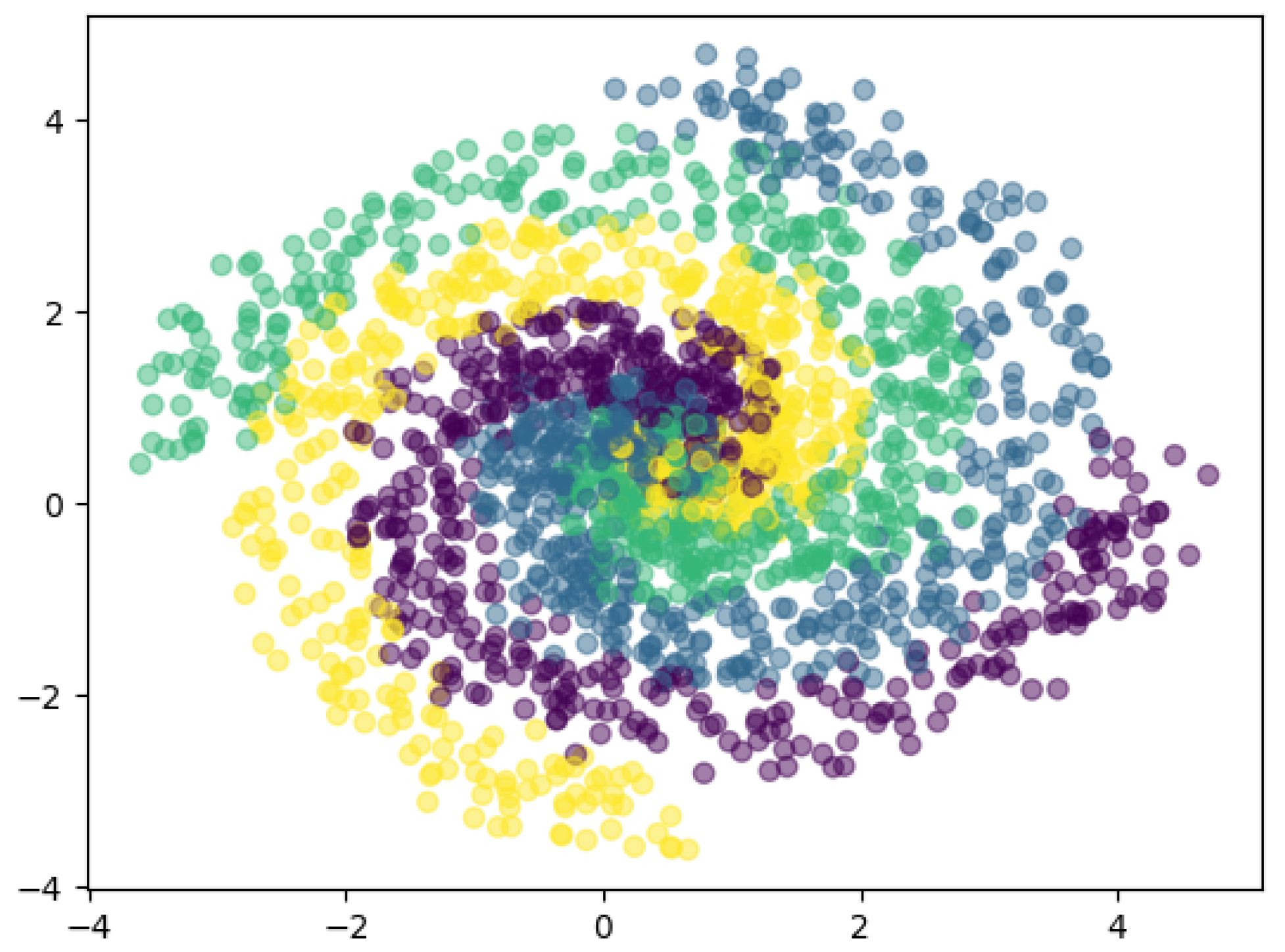
The spiral dataset under study is a synthetic, four-class dataset where each class forms a concentric spiral in the Cartesian plane. The selection of this dataset is primarily due to its non-linear and non-separable nature, which presents a challenging scenario for many learning algorithms and hence is more representative of real-world problems. The Cartesian coordinates $(x,y)$ of each point in the dataset are given by:

$$x=r·cos\left(\theta \right)$$

(1)

$$y=r·sin\left(\theta \right)$$

(2)

where r represents the distance from the origin and $\theta$ is the angle from the positive x-axis. The class of a point is determined by the number of full rotations $\varphi$ that $\theta$ makes around the origin. For example, if $\varphi \in [0,1)$, the point belongs to the first class; if $\varphi \in [1,2)$, the point belongs to the second class, and so on. The spirals are defined, such that the points of each class are densely located near the corresponding spiral, as depicted in Figure 1.

This preliminary study serves as a foundation for the subsequent sections by providing insights into the behaviors of different supervised learning algorithms under challenging conditions. It sets the stage for the application of these algorithms in the context of fraud detection on imbalanced datasets, where the inherent complexity and non-linearity of the data present similar challenges as the spiral dataset.

2.1. Supervised Learning Algorithms

2.1.1. Gaussian Naive Bayes

The Gaussian Naive Bayes classifier assumes that the likelihood of the features $x_1,x_2,\cdots ,x_n$ given a class y is Gaussian:

$$P\left(x_o\right|y)=\frac{1}{\sqrt{2\pi {\sigma }_y^2}}exp\left(-\frac{{(x_o-{\mu }_y)}^2}{2{\sigma }_y^2}\right)$$

(3)

where ${\mu }_y$ is the mean of the features for class y and ${\sigma }_y^2$ is the variance.

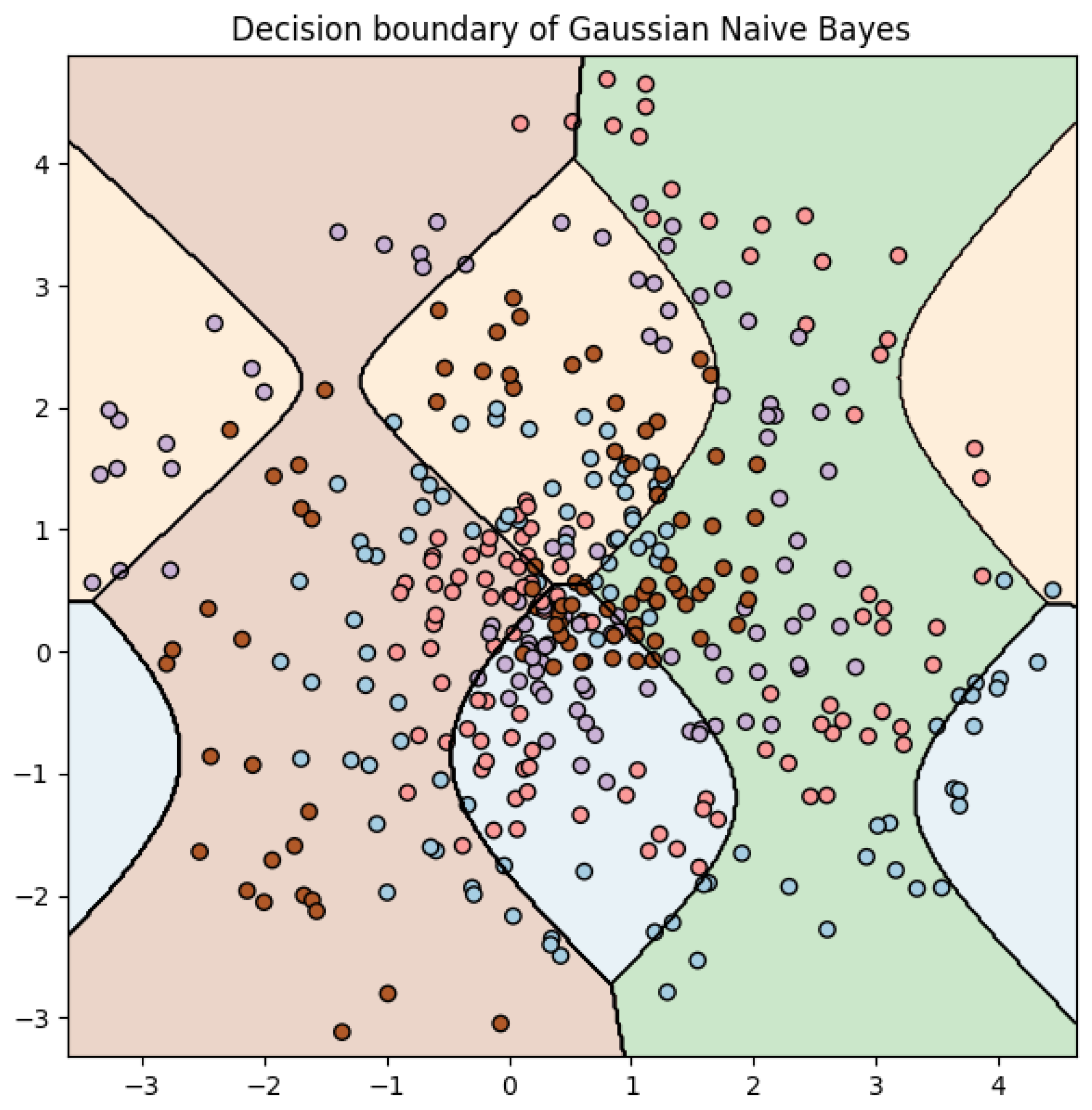
For Gaussian Naive Bayes, the decision boundaries are very complex due to the assumption that all features are conditionally independent given the class. This is a strong (and often not entirely correct) assumption, which does not work well for the spiral dataset, where the class labels are highly dependent on the combination of features rather than individual features.

From the accuracy scores (see

Table 1. Training and test accuracies for Gaussian Naive Bayes.

Training Accuracy	0.294375
Test Accuracy	0.2475

) and the confusion matrix (see

Table 2. Confusion matrix for Gaussian Naive Bayes.

	Predicted Class
	Class 1	Class 2	Class 3	Class 4
Actual Class 1	15	27	27	33
Actual Class 2	32	37	10	31
Actual Class 3	32	35	23	9
Actual Class 4	18	23	24	24

), we find that Gaussian Naive Bayes does not perform very well on this dataset. The accuracy on the test set is around 24.75%, which is low. The confusion matrix also indicates a significant number of misclassifications. Given the nature of the dataset (spirals), this is not surprising. The data are not linearly separable and the conditional independence assumption of Naive Bayes is violated because the class positions are highly dependent on both x and y coordinates together.

Our results suggest that Naive Bayes struggles with this type of problem, mainly due to its underlying assumptions, as shown in Figure 2. Naive Bayes assumes feature independence and generally performs well when this assumption holds. However, in the case of the spiral dataset, this assumption is violated since the x and y features are not independent given the class label.

Despite these limitations, Naive Bayes still has its merits. It is a simple and efficient algorithm that performs remarkably well on large datasets and in situations where the feature independence assumption is reasonably met. Examples of these situations include spam email detection, where the presence of certain words (features) are relatively independent of each other, and certain types of medical diagnosis problems, where symptoms can often be considered independent.

2.1.2. Linear and Quadratic Discriminant Analysis

Linear discriminant analysis (LDA) and quadratic discriminant analysis (QDA) are statistical classifiers. They assume that the observations from each class are drawn from a Gaussian distribution, and they estimate the parameters of this distribution. The decision boundaries are linear for LDA and quadratic for QDA.

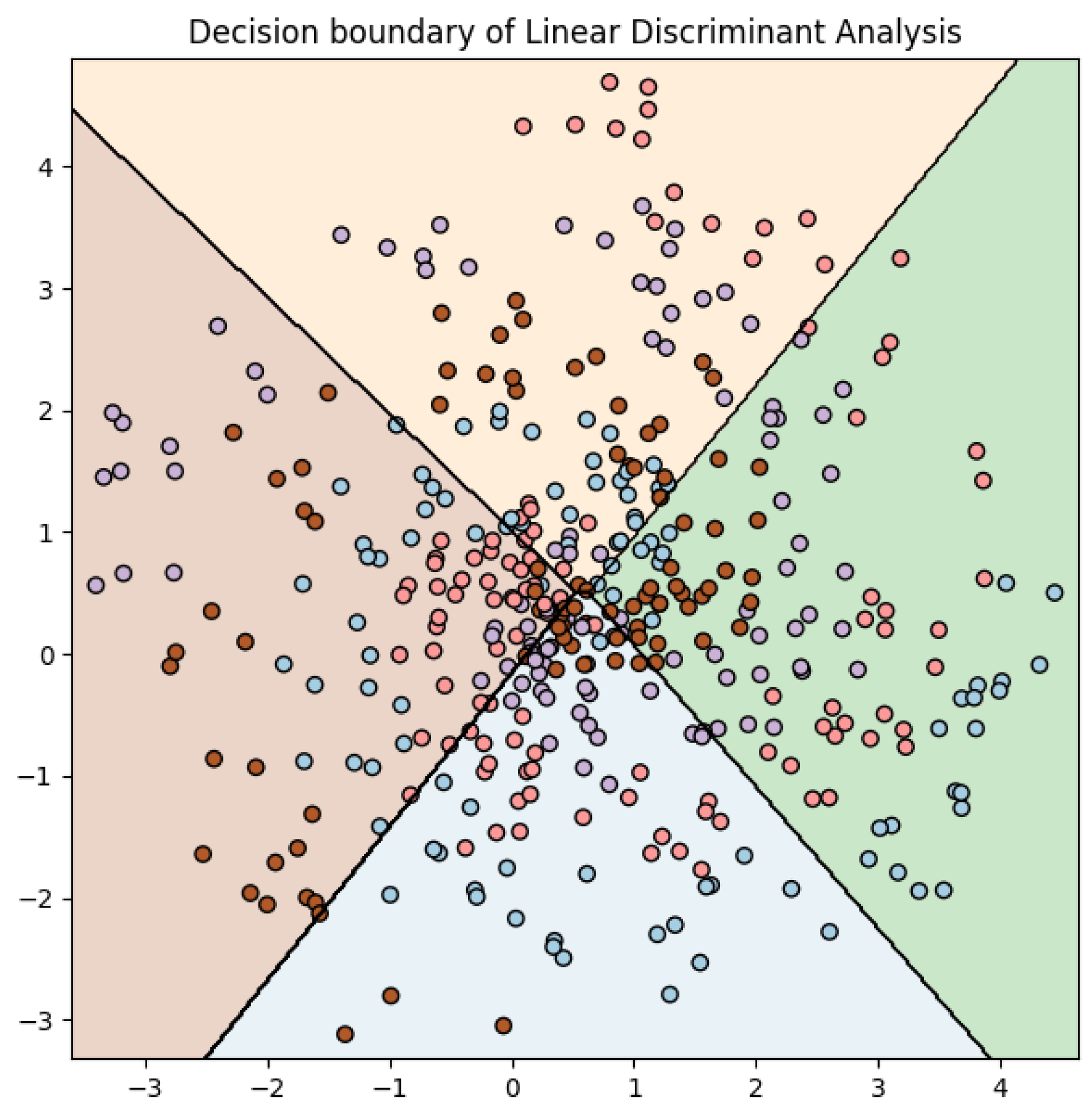
The decision boundaries of a linear discriminant analysis (LDA) classifier are linear because LDA is a linear method. These boundaries are determined by the means and variances of the features within each class. LDA tries to find a decision surface that maximizes the distance between the means of the classes and minimizes the variance within each class. However, for the spiral dataset, linear decision boundaries are not suitable due to the intertwined nature of the two classes.

From the accuracy scores (see

Table 3. Training and test accuracies for linear discriminant analysis (LDA).

Training Accuracy	0.255
Test Accuracy	0.2475

) and the confusion matrix (see

Table 4. Confusion matrix for linear discriminant analysis (LDA).

	Predicted Class
	Class 1	Class 2	Class 3	Class 4
Actual Class 1	24	29	24	25
Actual Class 2	27	27	21	35
Actual Class 3	27	28	24	20
Actual Class 4	17	25	23	24

), we find that the LDA classifier does not perform well on this dataset. The accuracy on the test set is approximately 24.75%, which is low. The confusion matrix also indicates a significant number of misclassifications.

This is to be expected as the spiral dataset is not linearly separable, and LDA is a linear method. The poor performance here suggests that the assumptions made by LDA (such as the Gaussian distribution of the classes and equal covariance matrices) do not hold for this dataset, as shown in Figure 3. Specifically, the linearity assumption of LDA does not work well with the spiral structure of this dataset.

The decision boundaries of a quadratic discriminant analysis (QDA) classifier are quadratic because, unlike LDA, QDA does not assume that the covariance of each class is identical. This allows the classifier to model quadratic decision boundaries, thus enabling it to model more complex relationships between the features.

From the accuracy scores (see

Table 5. Training and test accuracies for quadratic discriminant analysis (QDA).

Training Accuracy	0.26375
Test Accuracy	0.215

) and the confusion matrix (see

Table 6. Confusion matrix for quadratic discriminant analysis (QDA).

	Predicted Class
	Class 1	Class 2	Class 3	Class 4
Actual Class 1	28	13	33	28
Actual Class 2	40	18	11	41
Actual Class 3	38	36	19	6
Actual Class 4	16	29	23	21

), we find that the QDA classifier does not perform very well on this dataset. The accuracy on the test set is approximately 21.5%, which is quite low. The confusion matrix also indicates a significant number of misclassifications. This is likely due to the fact that, although QDA can model more complex relationships than LDA, it may still struggle with the spiral structure of the dataset, as depicted in Figure 4, which is even more complex.

2.1.3. K-Nearest Neighbors

The K-nearest neighbors (K-NN) algorithm assigns a point x to the class that is most common among its k-nearest neighbors. The distance between two points x and y is computed using the Euclidean distance:

$$d(x,y)=\sqrt{\sum _{o=1}^n{(x_o-y_o)}^2}$$

(4)

The results of the hyperparameter search shown in Figure 5 show that the K-nearest neighbors (K-NN) classifier, with k set to 15, provides the best accuracy on this dataset. It is noteworthy that the performance of the model improved significantly compared to when k was set, for instance, to 2, as seen by the increase in both the training and test accuracies.

This makes sense as K-NN is a non-parametric method, meaning it does not make any assumptions about the underlying distribution of the data. By increasing the number of neighbors considered, the model becomes more resilient to noise and outliers in the data, leading to a better generalization performance on unseen data.

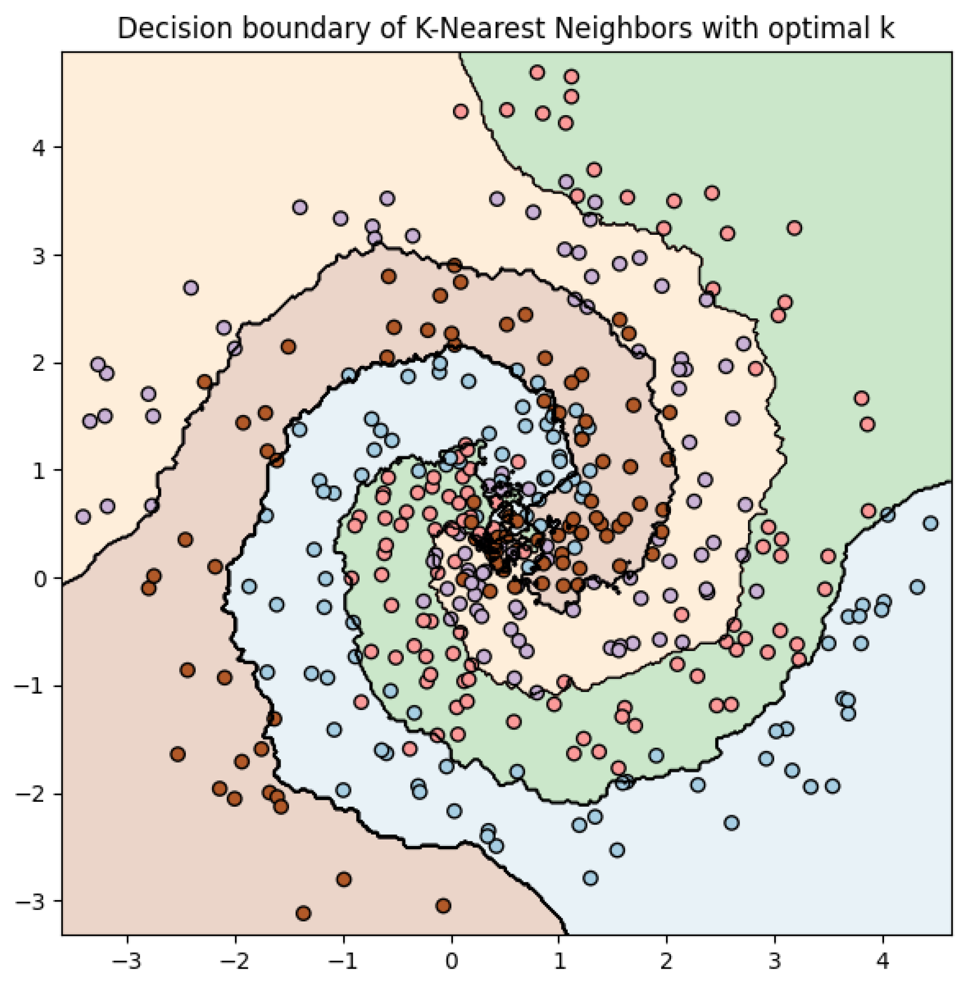
Graphically, the decision boundary becomes smoother with an increase in k. This is expected, as the decision of a larger number of neighbors tends to result in a more “consensus”-based decision, reducing the variance of the model and making the decision boundaries less susceptible to individual noisy instances.

The decision boundaries depicted in Figure 6 for K-NN with k equal to 15 are complex, as this algorithm has the flexibility to adapt to the complex structure of the data. This makes sense, given the intertwined spiral shapes of the data, which cannot be easily separated by a linear or simple non-linear boundary.

The predictions obtained on the test set are quite accurate, with a test accuracy of 0.79, see

Table 7. Training and test accuracies for K-nearest neighbors (K-NN) with k = 15.

Training Accuracy	0.83125
Test Accuracy	0.79

. The confusion matrix, see

Table 8. Confusion matrix for K-nearest neighbors (K-NN) with k = 15.

	Predicted Class
	Class 1	Class 2	Class 3	Class 4
Actual Class 1	75	9	2	16
Actual Class 2	8	93	9	0
Actual Class 3	5	7	82	5
Actual Class 4	10	3	10	66

, shows good performance across all classes, indicating that the K-NN model with k equal to 15 is capable of effectively classifying points in this spiral dataset.

2.1.4. Support Vector Machines

Support vector machines (SVMs) find the hyperplane that maximizes the margin between the two classes. The decision function is given by:

$$f\left(x\right)={\mathbf{w}}^T\varphi \left(x\right)+b$$

(5)

where $\varphi \left(x\right)$ is the feature vector, $\mathbf{w}$ is the weight vector, and b is the bias term.

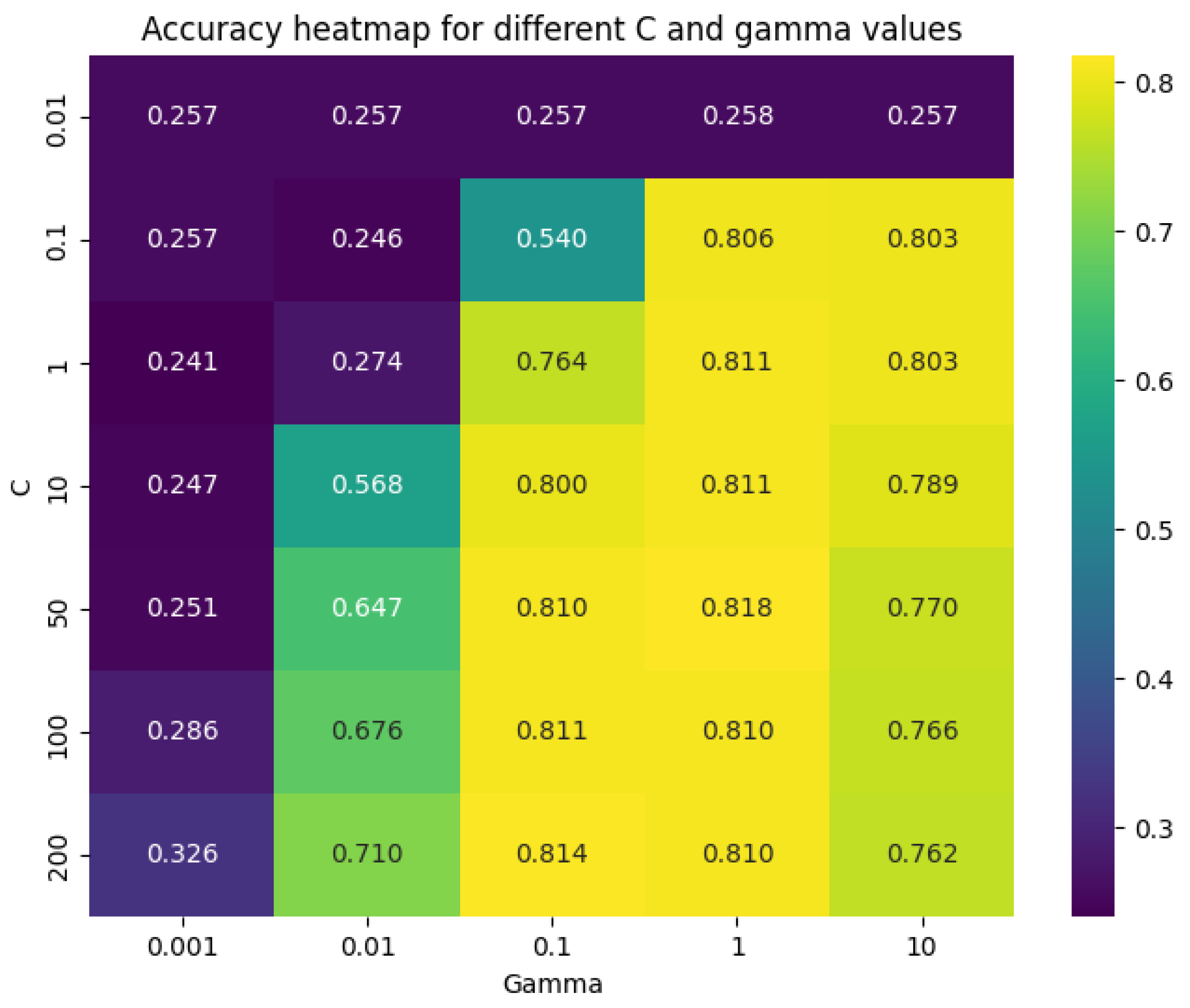
The search for the best hyperparameters for the SVM resulted in a C of 50 and a gamma of 1, as shown in Figure 7. The C parameter controls the trade-off between achieving a high classification accuracy on the training data and maximizing the margin of the decision boundary. In this case, a C of 50 means that the model leans more towards correctly classifying all training examples, even if it means having a smaller margin, which might lead to a more complex decision boundary.

The gamma parameter defines how far the influence of a single training example reaches. With a value of 1, the influence of the training examples does not reach very far; hence, the model is quite flexible and can adjust well to more complex decision boundaries.

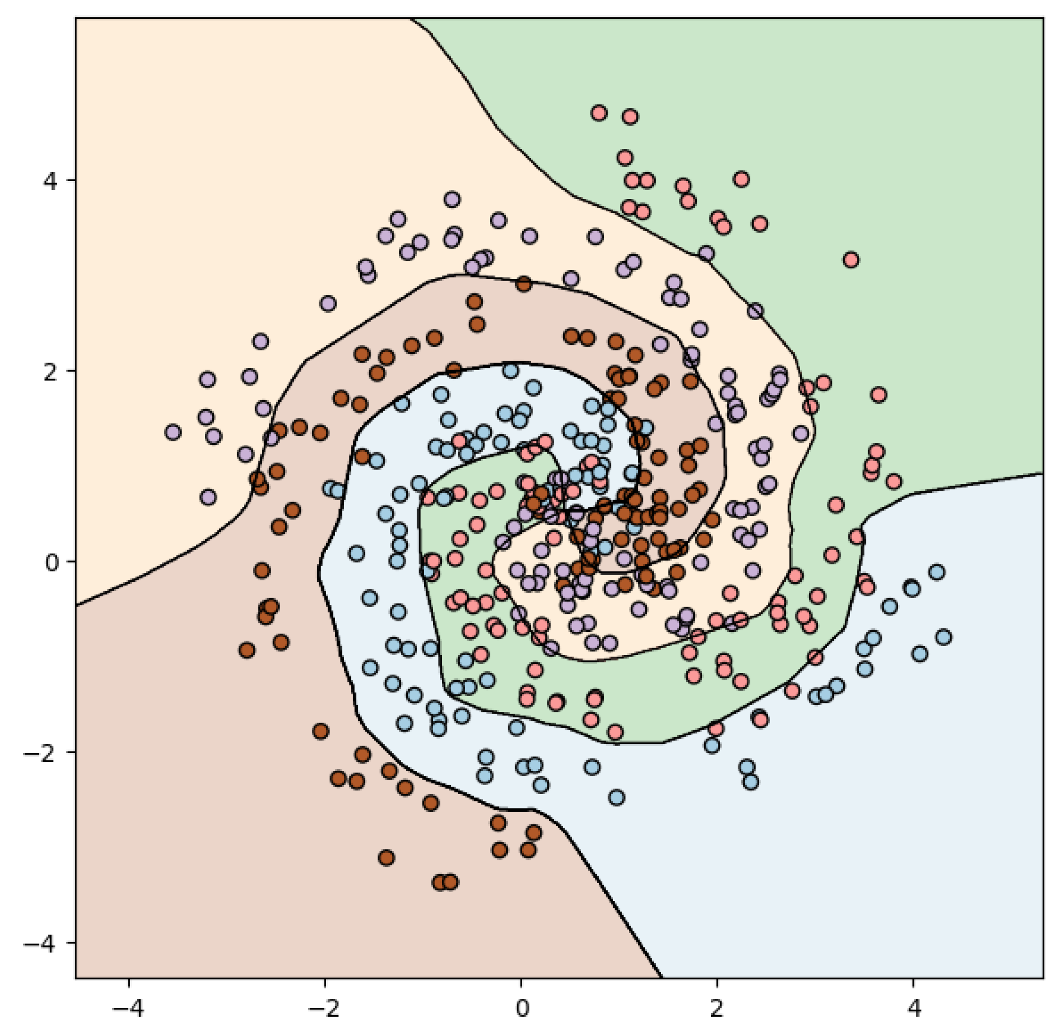
Looking at the decision boundaries, as depicted in Figure 8, they seem to make sense considering the SVM used. As we know, SVMs attempt to find the hyperplane that maximally separates the classes in the dataset. When the classes are not linearly separable, SVMs use a kernel trick to map the input into a higher-dimensional space where a hyperplane can be found. This is reflected in the decision boundaries, which appear to have been effectively drawn to separate the different classes.

The predictions on the test set were made by feeding the test set features into the trained SVM model. The model then uses the learned hyperplane to predict the class of each instance in the test set. The training accuracy is 85.25% and the test accuracy is 77%, see

Table 9. Training and test accuracies for support vector machines (SVMs) with C = 50 and gamma = 1.

Training Accuracy	0.8525
Test Accuracy	0.77

. This suggests that the model has learned the data quite well, but may be slightly overfitting given the drop in accuracy from the training set to the test set. However, the model still generalizes fairly well to unseen data, achieving a decent test accuracy. The confusion matrix (see

Table 10. Confusion matrix for support vector machines (SVMs) with C = 50 and gamma = 1.

	Predicted Class
	Class 1	Class 2	Class 3	Class 4
Actual Class 1	74	10	1	17
Actual Class 2	8	89	12	1
Actual Class 3	4	7	82	6
Actual Class 4	6	2	18	63

) further shows that the model has a balanced performance across different classes, albeit some classes are predicted better than others.

2.1.5. Decision Trees

Decision trees partition the feature space into regions. At each internal node of the tree, a decision is made based on a feature value, splitting the data accordingly. The process is repeated recursively.

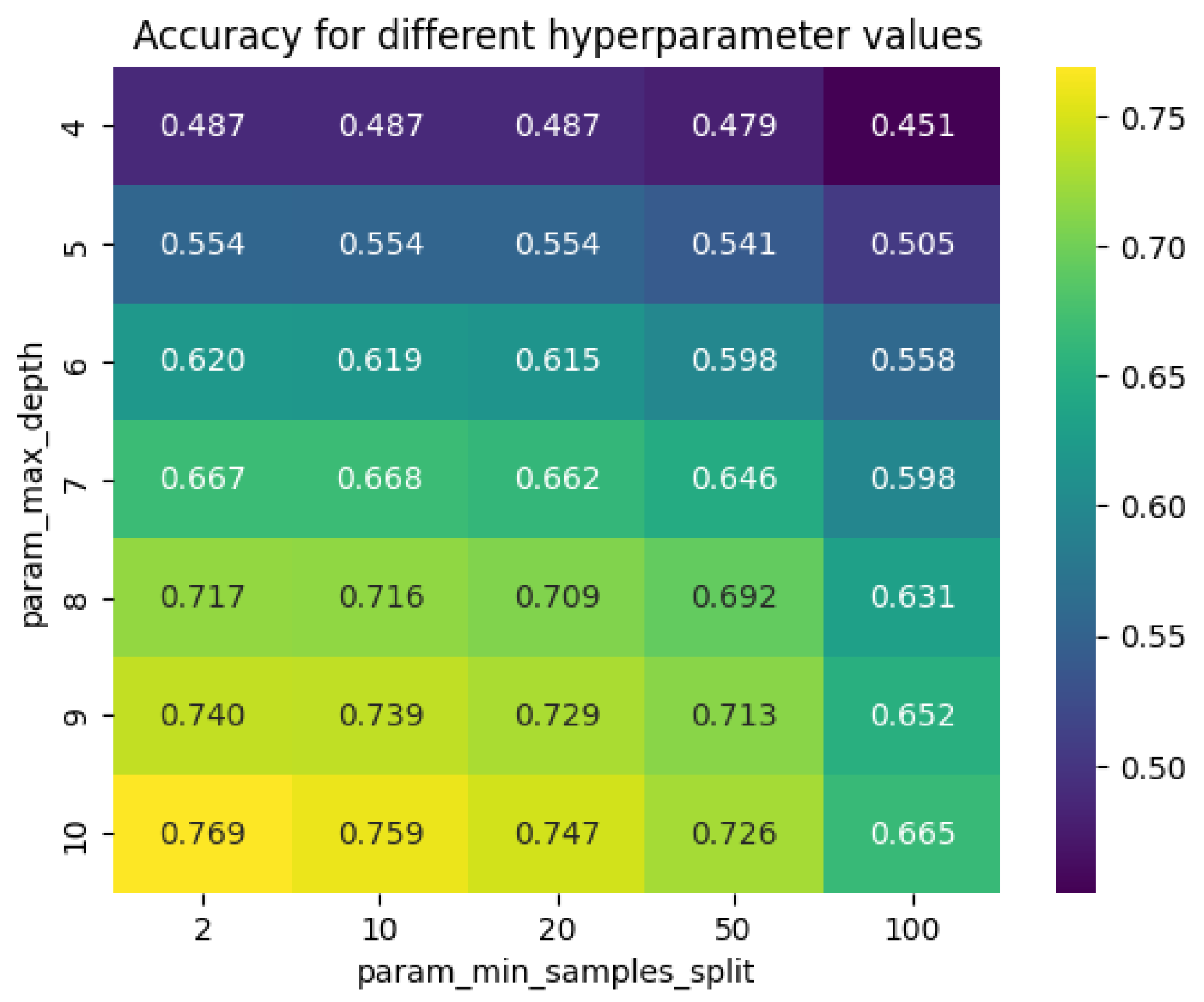
The search for the best hyperparameters, as shown in Figure 9, resulted in a maximum depth of 10 and a minimum sample split of 2. This means that the tree will have a maximum of 10 levels and a node will only be split if it contains at least 2 samples.

The decision boundaries in a decision tree are axis-aligned partitions of the feature space, i.e., all splits are perpendicular to an axis. This is because each decision in the tree is based on a single feature. In the plot, these decision boundaries appear as vertical and horizontal lines, dividing the space into regions, as can be seen in Figure 10 and Figure 11. Each region corresponds to a leaf of the decision tree and represents a class prediction.

Predictions on the test set are obtained by feeding the features of each test sample to the decision tree. The sample goes through the tree, with each decision based on one of its features, until it reaches a leaf node. The class associated with the leaf node is the prediction of the decision tree for that sample.

The accuracy on the test set is lower than on the training set, which indicates that the model may be overfitting the training data to some degree, despite the hyperparameter tuning; see

Table 11. Training and test accuracies for decision trees with max_depth = 10 and min_samples_split = 2.

Training Accuracy	0.854375
Test Accuracy	0.6975

. Overfitting occurs when the model learns the noise in the training data, causing it to perform poorly on unseen data. The confusion matrix (see

Table 12. Confusion matrix for decision trees with max_depth=10 and min_samples_split=2.

	Predicted Class
	Class 1	Class 2	Class 3	Class 4
Actual Class 1	66	10	10	16
Actual Class 2	9	71	30	0
Actual Class 3	0	7	85	7
Actual Class 4	8	0	24	57

) shows how the model’s predictions on the test set distribute across different classes. It can be seen that the model does a fair job as most of its predictions are correct (the diagonal elements), but there are still a good number of misclassifications (the off-diagonal elements).

2.1.6. Multi-Layer Perceptron

Toward the end of this preliminary study, we implemented an MLP model to classify the spiral dataset. While the decision tree and SVM approaches provided valuable insights, they can be limited in their ability to handle highly complex and non-linear data. The MLP, on the other hand, is a type of artificial neural network model that can approximate complex mappings from inputs to outputs. Its ability to handle non-linearity makes it a potent tool for this dataset.

An MLP consists of at least three layers of nodes: an input layer, a hidden layer, and an output layer. Each node in one layer connects with a certain weight to every node in the following layer. We used an MLP with 4 hidden layers, each comprising 20 neurons.

Given an input vector $x=(x_1,x_2,\dots ,x_n)$, the model applies a series of transformations, typically affine transformations followed by an activation function. An affine transformation is of the form $z=Wx+b$, where W is a matrix of weights and b is a bias vector. The activation function introduces non-linearity into the model. Common choices include the rectified linear unit (ReLU), which we use in our model, defined as $f\left(x\right)=max(0,x)$.

Our model is trained using the backpropagation method and the Adam optimization algorithm, a method for stochastic gradient descent. The model learns the optimal weights and biases that minimize the cross-entropy loss function, given by $L=-{\sum }_o{y}_{o}log\left(p_o\right)$, where $y_o$ denotes the true labels and $p_o$ represents the predicted probabilities.

Table 13. Training and test accuracies for multi-layer perceptron.

Training Accuracy	0.819
Test Accuracy	0.812

provides the training and test accuracies of the MLP model. The achieved training accuracy is 0.819, and the test accuracy is 0.812. These results indicate that our model exhibits good generalization and avoids overfitting to the training data.

The confusion matrix for the MLP model is shown in

Table 14. Confusion matrix for multi-layer perceptron.

	Predicted Class
	Class 1	Class 2	Class 3	Class 4
Actual Class 1	74	11	0	9
Actual Class 2	12	77	7	0
Actual Class 3	1	10	88	8
Actual Class 4	3	5	9	86

. The model demonstrates balanced performance across different classes, with no single class significantly outperforming or underperforming others.

Figure 12 visualizes the decision boundaries of our MLP model. As seen, the model is capable of drawing highly non-linear decision boundaries, allowing it to correctly classify the majority of the samples from the spiral dataset.

In summary, the MLP is a powerful tool for this task, thanks to its flexibility and ability to model non-linear decision boundaries. The use of MLP not only enriches our understanding of the data but also sets the stage for future exploration using more advanced deep learning techniques.

In our study, we determined that 20 neurons per layer struck a fine balance between the computational efficiency and model performance for our dataset. It is important to note that while we appreciate that further optimization of this parameter could potentially augment the model’s performance, our extensive hyperparameter tuning, including techniques such as grid search or random search, yielded marginal enhancements, particularly considering the escalation in model complexity. Therefore, our chosen architecture stands as a compelling baseline, offering noteworthy results with a manageable level of computational demand.

3. Resampling Techniques

In ML, resampling techniques are often employed to handle imbalanced datasets, where the number of instances across different classes is disproportionately distributed. There are three common resampling techniques, namely undersampling [21], oversampling [22], and SMOTE [8].

Undersampling is a technique designed to balance the class distribution by randomly eliminating majority class examples. This is done until the majority and minority class instances are balanced out. Mathematically, if we have a dataset D composed of two classes, i.e., the majority $C_{majority}$ and the minority $C_{minority}$, undersampling reduces the size of $C_{majority}$ to be equivalent to the size of $C_{minority}$.

Let $n_{majority}$ and $n_{minority}$ represent the number of instances in $C_{majority}$ and $C_{minority}$, respectively. Undersampling randomly selects $n_{minority}$ instances from $C_{majority}$ to produce a new majority class $C_{majority}^{\prime }$, such that $|C_{majority}^{\prime }|=|C_{minority}|$.

Oversampling, on the other hand, is a technique that adds more examples to the minority class. Oversampling is done by replicating the instances of the minority class to balance the class distribution. If we use the same notation as before, oversampling increases the size of $C_{minority}$ to be equivalent to the size of $C_{majority}$. Oversampling randomly selects instances from $C_{minority}$ with replacement to create a new minority class $C_{minority}^{\prime }$, such that $|C_{minority}^{\prime }|=|C_{majority}|$.

SMOTE is an oversampling method that creates synthetic samples from the minority class instead of creating copies. The minority class is oversampled by taking each minority class sample and introducing synthetic examples along the line segments, joining any/all of the k-minority class nearest neighbors.

Mathematically, for each instance in the minority class, the algorithm calculates the k-nearest neighbors. A sample is then chosen at random from these k neighbors, and a new instance is synthesized at a point along the line connecting the two instances. If we denote the instance in the minority class as $\overrightarrow{x}$, and the randomly chosen neighbor as $\overrightarrow{n}$, then the synthetic instance $\overrightarrow{s}$ is created as follows:

$$\overrightarrow{s}=\overrightarrow{x}+\lambda (\overrightarrow{n}-\overrightarrow{x})$$

where $\lambda$ is a random number between 0 and 1.

These resampling techniques provide a mechanism to balance the class distribution, which is a critical step in preparing the dataset for training an ML model.

4. Methodology

4.1. Description of the Dataset

The dataset under study is a real-world credit card transaction dataset collected over a two-day period in September 2013 by European cardholders. The dataset is highly imbalanced, with only 0.172% of transactions marked as fraudulent. It consists of 284,807 examples with 30 features, with features V1 to V28 having been anonymized for privacy reasons. The “Time” feature represents the seconds elapsed between each transaction and the first transaction, and the “Amount” is the transaction amount. The “Class” feature represents the transaction class and is set to 1 in case of fraud, and 0 otherwise.

The frequency ratio of the class variable is highly imbalanced, as shown in

Table 15. Frequency of each class in the fraud detection dataset.

Class	Frequency
0	284,315
1	492

. There are significantly more non-fraudulent transactions (Class = 0) than fraudulent ones (Class = 1). This is typical in situations, such as fraud detection, where the event of interest is relatively rare compared to the normal situation.

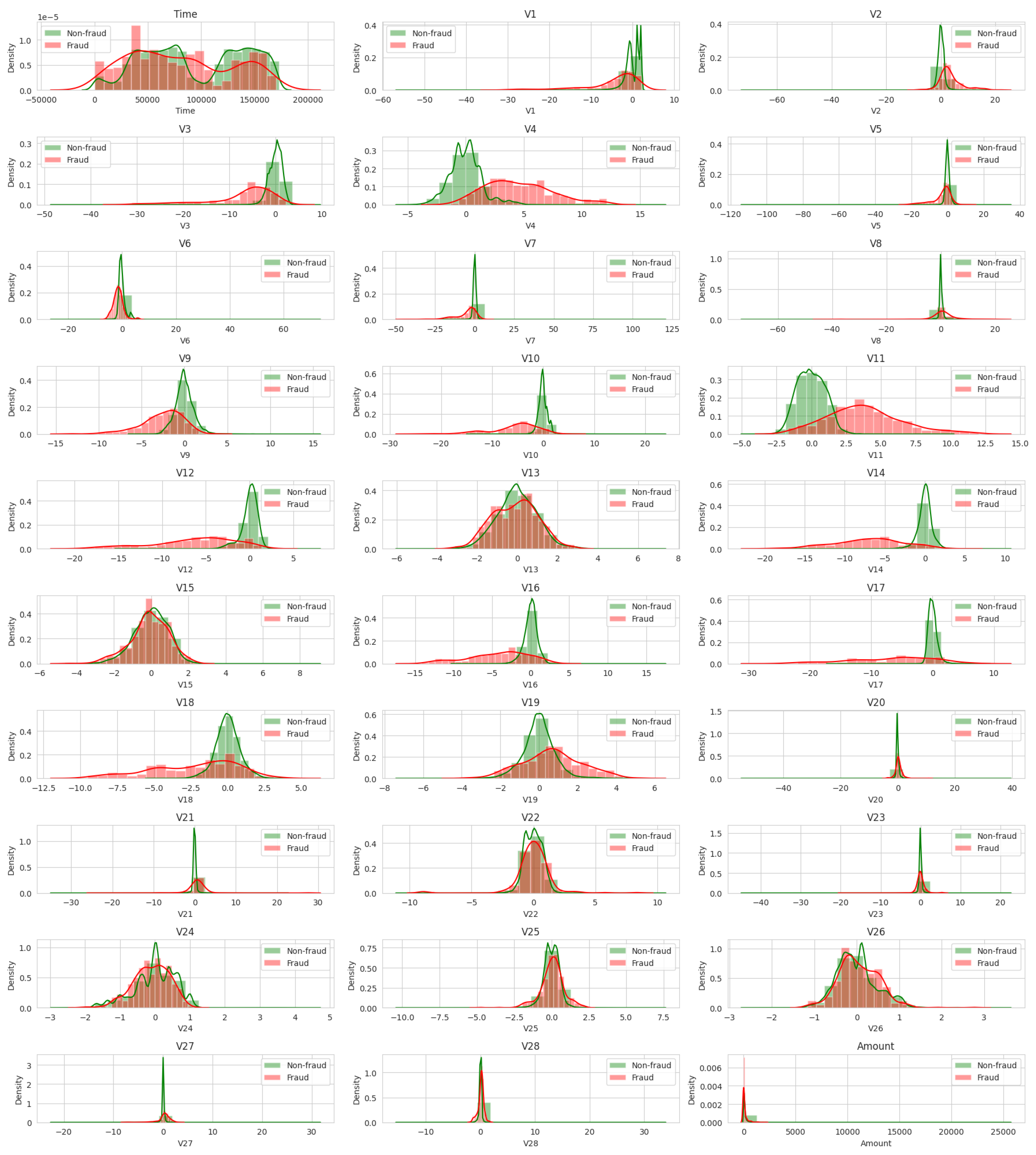
The histograms provide a distribution view of each feature, separated by class. This can give us insight into how each feature differs between fraudulent and non-fraudulent transactions. However, due to the high overlap and similar distributions of many features, it is difficult to identify clear patterns just from them. In order to better visualize the distribution of fraud versus non-fraud for each variable, we use normalized histograms, also known as density plots, where the area under the histogram integrates to 1, as seen in Figure 13. This allows us to compare the shapes of the distributions independent of the number of observations.

The preprocessing step involves scaling the “Amount” feature using StandardScaler from scikit-learn, which standardizes the feature by removing the mean and scaling to unit variance. The “Time” feature is dropped due to its negligible relevance to the problem of fraud detection.

4.2. Multilayer Perceptron (MLP)

Following the preliminary study of the spiral dataset, we adopted the MLP model for the main study on credit card fraud detection due to its robust performance in handling non-linear patterns and its versatility to fit complex data.

The spiral dataset posed challenges with its intrinsic interdependence between features and non-linear structure. The MLP, with its universal approximation property and ability to learn high-level abstractions, showed a significantly better ability to generalize from the complex, spiral dataset in our preliminary study, yielding promising results with a training accuracy of 0.819 and a test accuracy of 0.812 (as shown in Table 13).

Given that credit card fraud patterns may involve intricate relationships between diverse factors, it was logical to presume that the MLP’s proficiency in handling non-linear patterns, and in extracting high-level features, would serve well in detecting credit fraud. It offers the potential to understand non-linear and complex relationships between various factors in transaction data. Moreover, MLPs have the added benefit of being highly customizable, allowing us to tailor the network’s complexity to the problem under study.

The MLP is a class of feedforward artificial neural networks, which includes multiple layers of nodes in a directed graph. Each layer is fully connected to the next one. The MLP model used in this study consists of an input layer with a number of neurons equal to the number of features in the dataset, 4 hidden layers with 20 neurons each, and an output layer with 2 neurons, corresponding to the 2 classes of transactions, as illustrated in Figure 14. The neurons in the hidden layers use the rectified linear unit (ReLU) activation function, while the output layer neurons use the sigmoid activation function. The loss function used is binary cross-entropy.

The model is then compiled with the Adam optimizer (learning rate of 0.001) and binary cross-entropy loss function. The model is then fit to the training data for 100 epochs with a batch size of 2048, using 20% of the training data for validation. We also use EarlyStopping from keras.callbacks to stop the training when a monitored metric (in this case, validation loss) has stopped improving after 3 epochs, to prevent overfitting. Finally, we plot the training and validation loss and accuracy for each epoch to check the model’s learning progress.

The accuracy of the model on the test data is extremely high (99.94%), see

Table 16. Test accuracy and confusion matrix for MLP with four hidden layers and the Adam optimizer.

Test Accuracy

0.99937

, which initially appears to be an excellent result. However, given the imbalanced nature of the dataset (where the number of non-fraudulent transactions greatly exceeds the number of fraudulent ones), accuracy may not be the best metric to evaluate model performance.

The confusion matrix (see Table 17) provides more insights into the model’s performance:

• True negative (TN): 56,851, the model correctly predicted the non-fraudulent transactions.
• False Positive (FP): 13, the model incorrectly predicted these transactions as fraudulent.
• False Negative (FN): 23, the model incorrectly predicted these fraudulent transactions as non-fraudulent.
• True Positive (TP): 75, the model correctly identified these transactions as fraudulent.

Table 17. Confusion matrix for MLP.

	Predicted: No Fraud	Predicted: Fraud
Actual: No Fraud	56,851	13
Actual: Fraud	23	75

Table 17. Confusion matrix for MLP.

	Predicted: No Fraud	Predicted: Fraud
Actual: No Fraud	56,851	13
Actual: Fraud	23	75

While the number of false positives is low, the number of false negatives is concerning in this context. A false negative means a fraudulent transaction is undetected, which is a significant issue in fraud detection.

That is, it is critical to note that the problem of credit card fraud detection involves severely imbalanced classes, a challenge we must be mindful of. While our MLP model achieved a high test accuracy of 99.94% (refer to Table 16), we should treat this result cautiously due to the dataset’s skewed nature. Thus, other metrics, such as precision, recall, and the confusion matrix (Table 17), may provide a more comprehensive view of our model’s performance.

In this study, the hyperparameters for the conducted analysis were selected with an emphasis on establishing a strong baseline performance across the investigated techniques. Despite the good performance demonstrated by our chosen parameters, we acknowledge the critical role of extensive hyperparameter tuning in maximizing model performance. Therefore, in practical applications, a more thorough fine-tuning process is advisable to potentially achieve superior results.

4.3. Resampling Strategies

Undersampling involves randomly removing examples from the majority class, which can lead to a loss of information. This is compensated for by a more balanced dataset that could potentially improve the performance of the MLP.

Oversampling involves randomly duplicating examples from the minority class. Although this can lead to overfitting due to the exact replication of minority examples, it provides a more balanced dataset for the MLP.

SMOTE generates synthetic examples from the minority class. It selects two or more similar instances (using a distance measure) and perturbs each instance one attribute at a time by a random amount within the difference to the neighboring instances.

5. Experiments and Results

Our study’s primary objective was to develop a robust baseline model that exhibits exceptional performance; we also aimed to assess the efficacy of various resampling strategies, especially in reducing the rate of false negatives. In the context of fraud detection, minimizing the potential for not detecting fraudulent transactions is a critical operational requirement. Thus, our focus was to scrutinize this aspect while evaluating distinct resampling strategies.

In order to assess the impact of different resampling strategies on the performance of the MLP model, experiments were conducted with undersampling, oversampling, and SMOTE. For each strategy, a version of the dataset was created and used to train the MLP model. Each model’s accuracy was then evaluated on the test set.

Resampling was done only on the training data to avoid information leakage from the test set. The aim was to create a model that generalizes well to unseen data. If we use information from the test set during the training process, it could lead to over-optimistic performance metrics during testing, and the model would not perform as well on truly unseen data. This is why it is crucial to keep the test data separate and untouched until the very end of the process.

Analyzing the results, the test accuracy seems quite high at approximately 98.5%, see

Table 18. Performance comparison of the MLP model on undersampled, oversampled, and SMOTE data.

Method	Non-Fraud (Train)	Fraud (Train)	Test Accuracy	True Negative	False Positive	False Negative	True Positive
Undersampling	394	394	0.9851	56,028	836	15	83
Oversampling	227,451	227,451	0.99928	56,844	20	21	77
SMOTE	227,451	227,451	0.99909	56,838	26	26	72

. However, looking at the confusion matrix, we can see that the model has a large number of false positives (836), which indicates that it incorrectly classifies many normal transactions as fraudulent. This is likely due to the fact that the model is trained on a balanced dataset (achieved through undersampling) and, thus, may overestimate the probability of fraud when applied to the original, highly imbalanced data. The corresponding training and validation accuracies and loss curves are shown in Figure 15 and Figure 16.

In terms of whether we can keep this model acceptable, it depends on the specific use case and the cost trade-off between false positives and false negatives. In a credit card fraud detection context, a false negative (fraudulent transaction classified as normal) could potentially cost the company a lot of money, while a false positive (normal transaction classified as fraudulent) would mainly cause inconvenience to the customer. However, if the number of false positives is too high, it may also lead to customer dissatisfaction and loss of trust in the company. Thus, while the overall accuracy of the model is high, its practical utility may be limited due to the high number of false positives.

The primary reason we only resample the training data is to prevent information leakage from the test set into the training set. Resampling techniques, such as oversampling and undersampling, involve creating synthetic samples or choosing specific samples based on the existing data [10,12]. If we were to include the test set in our resampling, the model might gain information from the test set during training, which would give us an overly optimistic and potentially misleading measure of how well our model generalizes to unseen data [23].

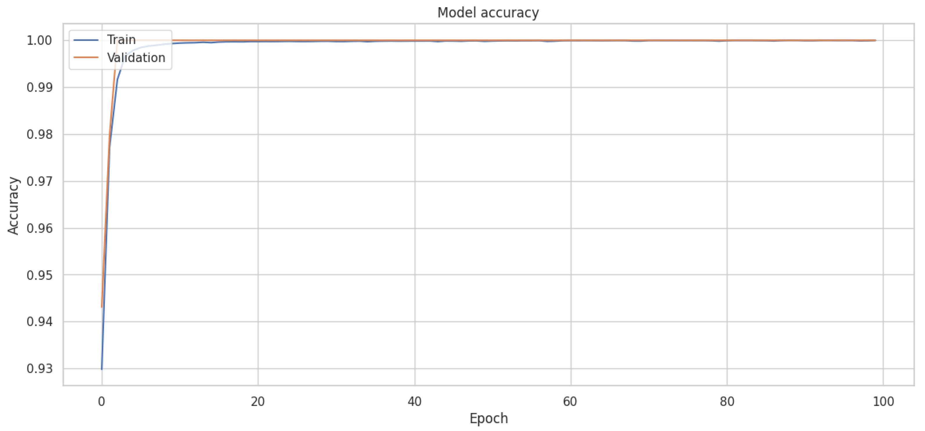
The results from oversampling show a very high accuracy of 99.93% on the test set, as can be seen in Table 18. The confusion matrix indicates that the model has a very high true positive rate and a very low false positive rate, which is desirable in this context. However, in the context of fraud detection, it is also important to minimize the number of false negatives (fraudulent transactions that are classified as non-fraudulent). In this case, there are 21 false negatives, which might be considered too high, depending on the context and the cost associated with missing a fraudulent transaction. The corresponding training and validation accuracies and loss curves are shown in Figure 17 and Figure 18.

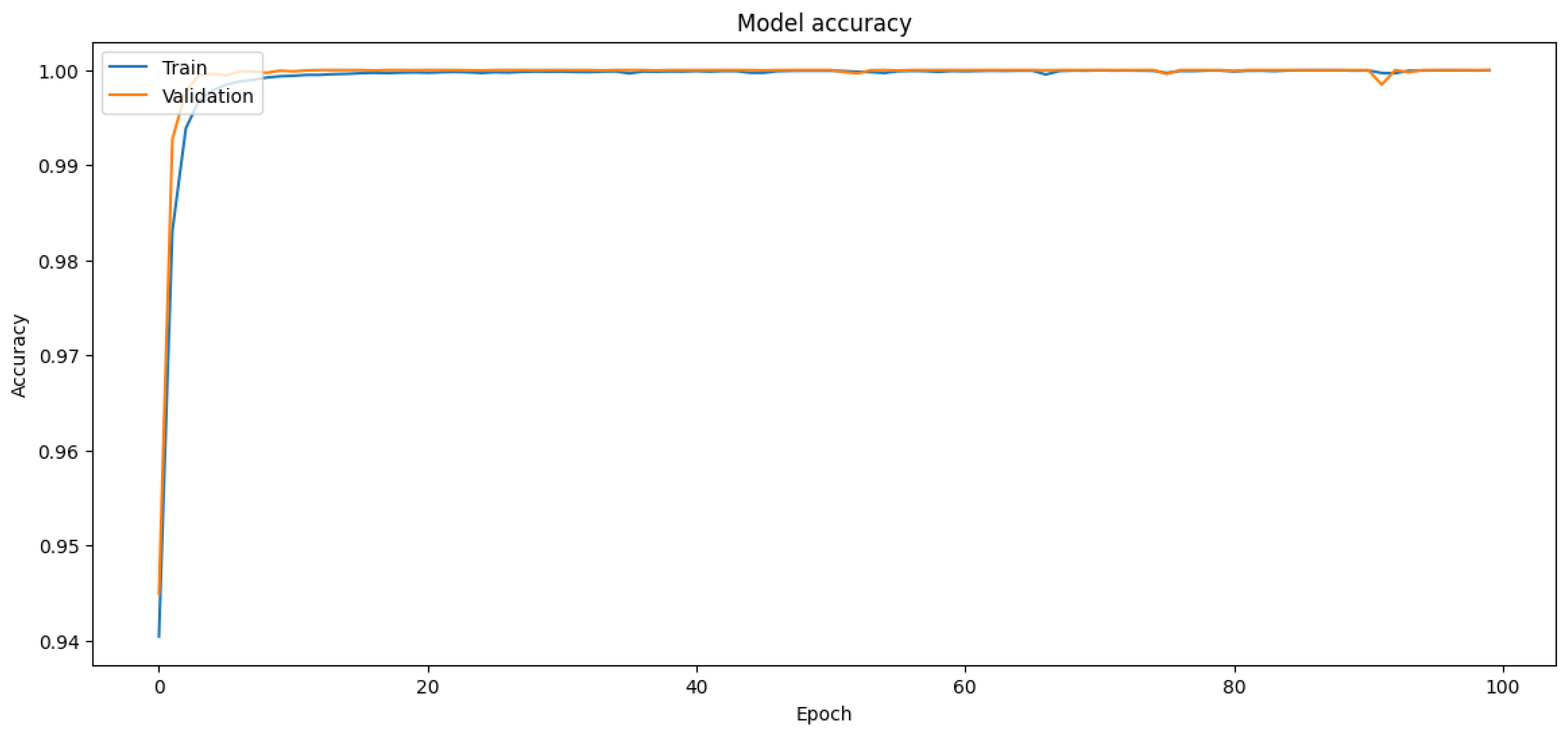
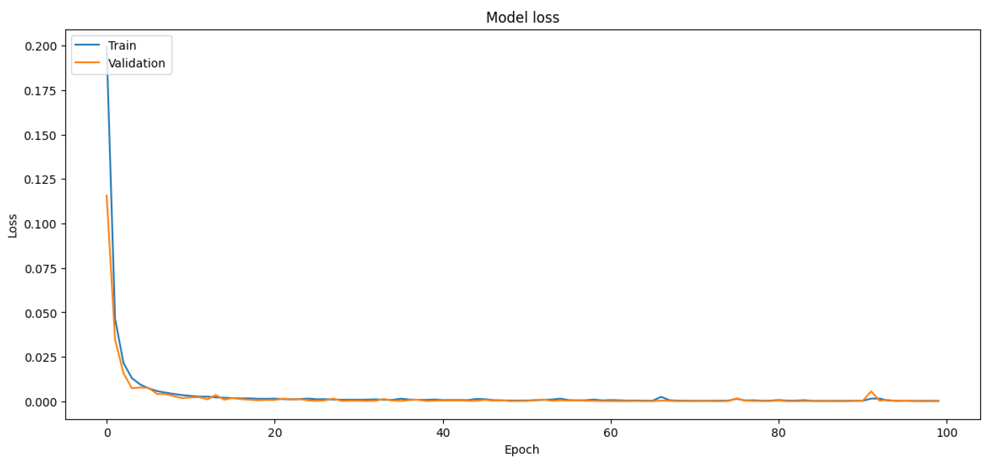
In this case, SMOTE is applied to the training set. Using the entire dataset is an acceptable approach when the dataset is highly imbalanced. However, there is a potential pitfall to keep in mind: synthetic samples could be created based on information from the future (test set), which is a form of data leakage that can lead to overly optimistic performance estimates. The best practice is usually to apply SMOTE (or any other form of resampling) during cross-validation within the training set, and not on the test set or the entire dataset.

The test accuracy of the model trained with SMOTE is slightly lower than the model trained without SMOTE, as shown in Table 18. However, accuracy alone can be a misleading measure, particularly in the context of imbalanced datasets. It is important to look at the confusion matrix as well. We see that the model with SMOTE has a slightly higher number of false positives (non-fraudulent transactions that were classified as fraudulent) and false negatives (fraudulent transactions that were classified as non-fraudulent). Depending on the costs associated with false positives and false negatives, one model might be preferred over the other. The choice of the model will depend on the specific business context and the trade-off between precision and recall. The corresponding training and validation accuracies and loss curves are shown in Figure 19 and Figure 20.

In this particular case, cross-validation can be problematic due to the limited representation of the minority class. The traditional cross-validation strategy could potentially lead to folds where the minority class is very under-represented or even entirely absent, resulting in poor generalization of the trained model. In our research, we used oversampling to balance the dataset before splitting it into training and validation sets, and we ensured a substantial representation of the minority class in both the training and validation sets. It is worth noting that this oversampling was performed only on the training data, leaving the validation data untouched to provide a realistic evaluation of the model performance on imbalanced data and avoid data leakage. Hence, this approach effectively mimics the spirit of cross-validation while accommodating the special requirements of our imbalanced data. Lastly, we kept aside a separate test set, which was not involved in either training or validation processes, to evaluate the final performance of the models, ensuring an unbiased assessment of the generalization capability of our models.

We can provide the following analysis:

• Undersampling: This model, trained on a perfectly balanced dataset (with 394 instances each of fraud and non-fraud cases), shows a good overall test accuracy of 98.51%. However, it appears to have struggled more than the other models in correctly classifying cases, as indicated by the higher number of false positives (836). This means it incorrectly classified 836 normal transactions as fraudulent, which can lead to unnecessary alerts in a real-world fraud detection system; those are indeed annoying for the final user, but not critical.
• Oversampling: This model was trained on a significantly larger dataset (with 227,451 instances each of fraud and non-fraud cases). The test accuracy here is very high at 99.928%, and it performed well in terms of minimizing false positives (only 20) and false negatives (21). This shows that the oversampling model has excelled in correctly identifying both fraudulent and non-fraudulent transactions.
• SMOTE: Similar to the oversampling model, this model was trained on a large, balanced dataset (227,451 instances each). The test accuracy is very high at 99.909%, but it has slightly more false positives (26) and false negatives (26) compared to the oversampling model. This means that, while SMOTE has performed extremely well, it has slightly underperformed the oversampling model in this case.

In conclusion, while all models perform well, the oversampling model appears to provide the best results in this case, with the highest test accuracy of 99.928% and the lowest number of false positives (20/227,451) and false negatives (21/227,451). The undersampling model, while still performing admirably, struggles more with classifying transactions correctly. The SMOTE model performs almost as well as the oversampling model but falls just slightly short in terms of both accuracy and the number of incorrect classifications.

An important aspect to consider is that the SMOTE synthesizes new instances of the minority class by interpolating between existing examples. While this strategy can mitigate the overfitting issue that might occur with oversampling, where specific instances are simply replicated, SMOTE carries its own risk. Specifically, it may generate synthetic instances within regions of the feature space predominantly occupied by the majority class, thereby inadvertently introducing noise into the dataset. This noise introduction could plausibly explain why oversampling outperforms SMOTE in this specific context. An alternative approach could be to use SMOTE-ENN [23], which is an excellent technique that combines oversampling the minority (or under-represented) class instances using SMOTE and cleaning the resultant dataset using the edited nearest neighbor (ENN) algorithm. It could indeed help in handling the problem of noisy instances and borderline instances that SMOTE alone might struggle with, and could potentially yield better results.

Additionally, to further strengthen the work, the following strategies could be tested:

• Nested cross-validation: While standard k-fold cross-validation can indeed be problematic for imbalanced datasets, nested cross-validation could be used to further validate the generalizability of the model and the robustness of the results. In nested cross-validation, the outer loop is used to evaluate the model’s performance, while the inner loop is used to tune the model’s hyperparameters. This can provide a more unbiased estimation of the model performance and could address concerns about overfitting.
• Comparison with other resampling methods: While we already compared oversampling, undersampling, and SMOTE, there are other resampling methods that could be considered to broaden the scope of the work besides the already mentioned SMOTE-ENN. This could include methods such as ADASYN (adaptive synthetic sampling) [9], ROSE (random oversampling examples), or using distinct versions of SMOTE, such as Borderline-SMOTE [24] or SVM-SMOTE.
• Incorporating cost-sensitive learning: Since the focus of the study is on reducing false negatives (which is critical in fraud detection), incorporating cost-sensitive learning in the model could be a significant addition. This is a way to provide the model with more information about the relative importance or “cost” of different types of errors.

6. Discussion

The results of our experiments provide insights into the effectiveness of different resampling strategies when dealing with imbalanced datasets. The comparative analysis highlights the strengths and weaknesses of each approach. The best-performing model, in terms of accuracy and generalization, should be chosen based on careful consideration of the trade-offs between true positive rates, false positive rates, and model complexity.

One of the major advantages of the approach we have studied is its adaptability. By adjusting the resampling technique, it can be fine-tuned to deal with different levels of class imbalance, a common issue in fraud detection. Furthermore, through hyperparameter optimization, the performance of the MLP can be optimized for different types of datasets, making it suitable for a wide range of applications in mobile and ubiquitous technologies.

In all these applications, it is important to note that the effective implementation of our approach would require careful consideration of user privacy and data security issues. The design and use of these systems must comply with relevant data protection regulations and ethical guidelines, ensuring that personal and sensitive data are handled responsibly.

6.1. Performance and Scalability

A critical aspect of integrating ML models into mobile and ubiquitous systems is the consideration of performance and scalability. These factors determine the feasibility of deploying our proposed methods in real-world settings, particularly in systems with stringent resource constraints or high data throughput requirements.

The MLP model, despite its effectiveness in handling complex classification tasks, can be computationally intensive, especially with large datasets or complex architectures. However, several strategies can be employed to mitigate these computational demands. First, through careful hyperparameter tuning, we can optimize the trade-off between model complexity and performance, ensuring the MLP is as efficient as possible. Second, techniques such as model pruning or quantization can be employed post-training to reduce the computational resources required for inference without significantly compromising accuracy.

In terms of memory, the MLP model, similar to other neural networks, requires sufficient space to store weights and biases for each layer. For mobile or IoT devices with limited memory, this may pose a challenge. However, memory-efficient techniques, such as weight sharing or binary neural networks, can be explored to reduce the memory footprint of the MLP.

While our study employed a relatively large dataset, in a real-world setting, mobile banking or payment systems may deal with significantly larger volumes of data. The scalability of our approach to such datasets depends on several factors. Training an MLP on a larger dataset would require more computational resources and time. However, techniques such as distributed training, or the use of more powerful hardware, can be employed to handle larger datasets. Moreover, the use of mini-batch gradient descent during training allows for the model to be trained on larger datasets without requiring proportionally larger memory.

For real-time fraud detection in mobile or ubiquitous systems, the ability to process data and make predictions quickly is vital. After training, MLPs can make predictions relatively quickly, making them suitable for real-time applications. However, the speed of prediction can be influenced by factors such as model complexity and the dimensionality of the input data. Therefore, care must be taken during model design and data preprocessing to ensure that the system can meet the required latency for real-time processing.

6.2. Privacy Considerations

In the context of fraud detection, particularly in applications such as mobile banking or payment systems, privacy becomes a paramount concern. The resampling process, model training, and subsequent application must all be conducted in a manner that respects and preserves user privacy. In this section, we outline some of the key privacy considerations associated with our approach.

Resampling techniques, including undersampling, oversampling, and SMOTE, involve manipulating the original dataset to address the class imbalance. While these techniques do not inherently compromise privacy, care must be taken when implementing them. For example, in oversampling, duplicates of minority class instances are created. If these instances contain sensitive information, their duplication could potentially increase the risk of a privacy breach in case of data leakage. The synthetic samples generated by SMOTE, on the other hand, could be considered less privacy-intrusive, as they do not directly replicate existing instances, but instead create new, synthetic instances based on feature space similarities.

Training the MLP model requires access to user data, raising potential privacy issues. To mitigate this, techniques such as differential privacy can be employed. Differential privacy introduces a certain amount of noise to the data or the model’s outputs, ensuring that the inclusion or exclusion of any single data point does not significantly affect the results, thereby preserving individual privacy.

Additionally, to prevent potential privacy breaches during the model application phase, the principle of data minimization should be adopted. This principle dictates that only the minimum necessary data should be used for making predictions. By limiting the scope of data used in the model, we can ensure that we are not unnecessarily exposing sensitive information.

Finally, it is crucial to consider legal and ethical guidelines regarding data privacy, such as the General Data Protection Regulation (GDPR) in the European Union. These guidelines stipulate requirements for data consent, anonymization, and the rights of individuals, among other things. Adherence to these guidelines is not only a legal requirement, but also a means of ensuring ethical conduct in the handling of user data.

That is, while our proposed methodology offers promising results in addressing imbalanced data for fraud detection, it is essential to implement it in a privacy-preserving manner. By incorporating privacy measures at each step of the process, we can ensure that our approach is not only effective but also respects user privacy.

7. Conclusions

This study presented a comprehensive investigation of various supervised learning algorithms on a synthetic dataset based on four-class spirals. The findings are then applied to a real problem task of credit card fraud detection, where we achieve a state-of-the-art test accuracy of 99.937% using the MLP model to classify the synthetic data. Then, we observe the effects of using resampling strategies in order to reduce the number of false negatives; notice that this is particularly important for the task under consideration. Hence, we tested undersampling, oversampling, and SMOTE. The results demonstrate the importance of addressing the class imbalance in the data preprocessing phase to improve model performance. Our findings suggest that the choice of resampling strategy should be context-dependent, taking into consideration the specific characteristics of the dataset, and the trade-off between model accuracy and interpretability. In particular, we achieve a compelling overall accuracy of 99.928% using oversampling, with a significantly low number of false negatives (21/227,451).

In conclusion, while there is no one-size-fits-all solution to handle imbalanced data and non-linearity, a combination of carefully chosen resampling strategies and model hyperparameter tuning can lead to significant improvements in model performance.

Our contributions in this paper include a comprehensive exploration of methodologies for handling imbalanced datasets, with a focus on resampling strategies and their application in fraud detection. We demonstrate that our proposed approach, which combines a carefully selected ML model with tailored resampling strategies, significantly improves the detection of fraudulent transactions. Moreover, we highlight the critical importance of addressing privacy concerns when implementing such methods, underscoring the need for incorporating privacy measures into every step of the process. Thus, our work not only advances the state of the art in imbalanced data handling and fraud detection but also provides valuable guidance on integrating privacy considerations into the implementation of these methodologies.

Despite the experimentation and analysis conducted, this study has some limitations. The choice of hyperparameters explored may not cover the entire possible search space and, therefore, there may be room for further optimization. Moreover, the neural network architecture used in this study was limited to a specific type, the MLP. Other types of neural networks or ensemble methods might yield different results, and so should be considered in future work.

There are several avenues for future research to build upon the findings of this study. First, additional resampling techniques and variations of existing methods can be explored to determine their effectiveness in handling imbalanced data. Second, the impacts of different feature engineering and selection methods on model performance can be investigated. Lastly, while alternative ML methodologies, including DL architectures, could potentially be deployed to determine the optimal model for fraud detection within imbalanced datasets, it is crucial to consider the specific parameters of each use case. Indeed, the suitability of more sophisticated models will inevitably hinge on a range of factors such as computational resources at one’s disposal and the desired performance outcomes. Hence, it is vital to strike a balance between achieving superior predictive accuracy and managing computational demands efficiently.