The Hybrid Brake Model and Its Validation

Abstract

As an extension of a paper published at the 24th International Conference on Mechatronics Technology, ICMT 2021 conference, this paper shows the concept, design method, and model of a hybrid brake with additional validation. An eddy current brake cannot be used to decelerate a vehicle to a standstill. However, the magnetic attraction force between the rotor and stator of an eddy current brake can be used to generate an additional mechanical friction torque. By using a disc spring between the rotor and stator, the eddy current brake is extended to a so-called hybrid brake. In particular, the model and design method of the disc spring are the focus of this work. Using a system model that includes the electromagnetic and mechanical domains, the wear reduction compared to a conventional friction brake and the dynamic behaviour depending on the spring parameters are investigated. Finally, a disc spring is designed in FEM with the desired force–displacement curve. In addition, a working demonstrator of a hybrid brake is constructed, and the electromagnetic and mechanical system models are compared with the experimental results. For the first time, it is shown that the concept of using the magnetic attraction force between the rotor and stator of an eddy current brake for braking to a stop is working. In a speed range of 0–7500 rpm, it is possible to generate a torque of 100 Nm, whereby at speeds higher than 3500 rpm, the torque is generated in a wear-free manner by eddy currents. However, in order to be valid, the model must be extended to represent the deformation of the rotor.

1. Introduction

In the course of vehicle electrification, a large part of the braking energy to be converted can be recovered. However, a mechanical brake is still required for safety reasons. One reason is the need for a redundant system. Another reason is that the maximum required braking torque cannot be achieved with the electric drive system. For example, an ordinary electric vehicle with a mass of 1700 kg at a speed of 140 km/h requires a braking power of 713 kW if, for safety reasons, a grip value between the tire and the road of 1.1 is fully utilised. Thus, the required brake power for normal powered vehicles is 3 to 8 times higher than the nominal propulsion power. One way to further reduce the use of a friction brake subject to wear is to use a wear-free eddy current brake (ECB). However, state-of-the-art eddy current brakes have the following disadvantages:

• Very low power density compared to friction brakes;
• Braking to a standstill is not possible.

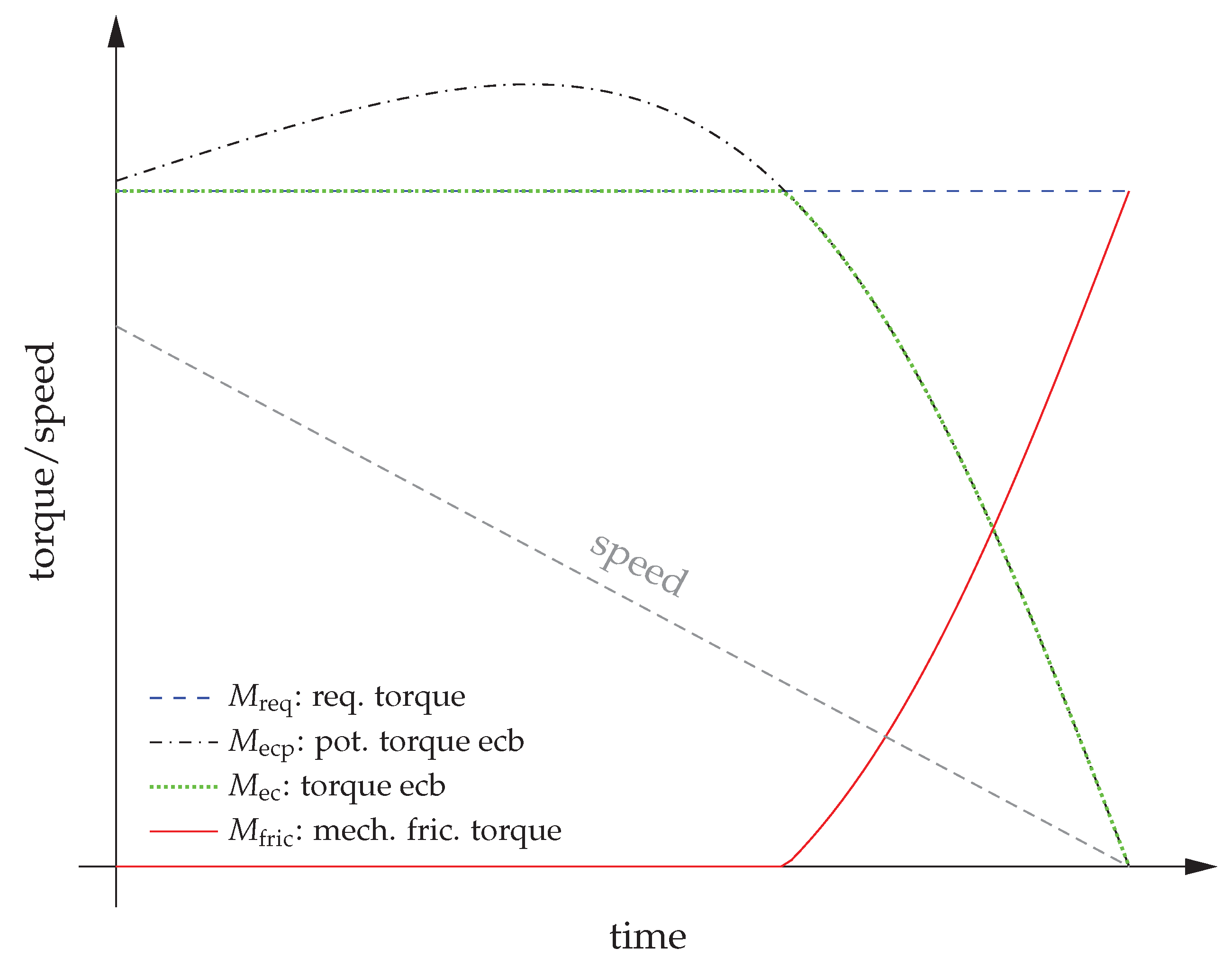
In [1], it is shown that the disadvantage of a low power density can be compensated for by using a magnetoisotropic material structure. This structure allows the skin effect to be reduced and increases the free cooling area. Figure 1 shows the braking torques in a braking process with a constant required torque $M_{\mathrm{req}}$ and linearly decreasing speed n when using an eddy current brake. At lower speeds, an additional mechanical friction brake must supply the difference between the required torque and the torque of the eddy current brake $M_{\mathrm{ec}}$ with a torque of $M_{\mathrm{fric}}$. Combinations of eddy current brakes and friction brakes have already been presented in other publications. In [2,3], concepts are presented in which the eddy current brake and the friction brake operate locally and separately. In other concepts [4,5], additional excitation poles are positioned on the brake disc to generate eddy currents and thus a wear-free portion of the braking torque. All of these concepts generate frictional torque via a classic brake caliper. However, the concept presented here and in a related patent [6] uses the magnetic attraction between the rotor with exciter poles and the stator of an eddy current brake to generate additional frictional torque, such as an electromagnetic friction brake [7,8]. An additional actuator with power electronics or even a hydraulic system is therefore not required. This work demonstrates, for the first time, the use of magnetic attraction between the rotor and stator of an eddy current brake to decelerate to a standstill. In addition to the work of [9], in this paper, measurement data for a functional demonstrator of the hybrid brake and the validation of the model are shown.

2. Concept of the Hybrid Brake

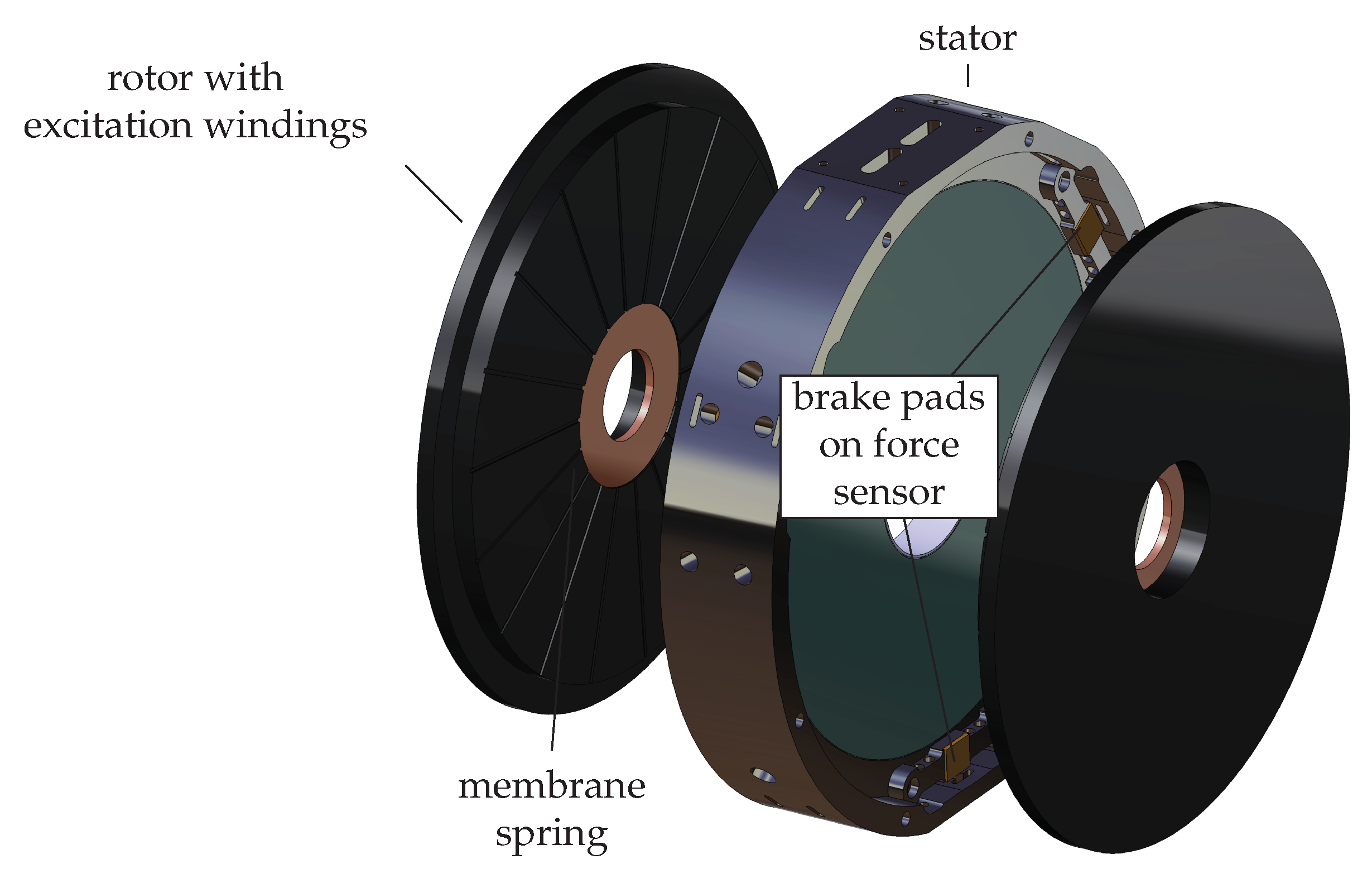
Figure 2a shows an exemplary cad model, and Figure 2b shows the superordinate operating principle of the hybrid brake. The current in the excitation windings on the rotor excites eddy currents in the stator, which generate an eddy current torque $M_{\mathrm{ec}}$ during the rotary motion.

At low speeds, the induction effect decreases sharply until, at zero speed, no braking torque is generated by eddy currents.

At these low speeds, the magnetic attraction force $F_{\mathrm{n}\mu }$ between the rotor and stator is used to generate a frictional torque $M_{\mathrm{fric}}$ to brake to a stop. Since contact between the rotor and stator is necessary for the frictional action, a spring is used to ensure that contact is not present when the hybrid brake is not required to provide a braking torque. Since the torque must be transmitted from the rotor to the hub and the rotor must be axially displaceable at the same time, a diaphragm spring is used.

3. Design Method

As with the eddy current brake, the hybrid brake is optimised for maximum wear reduction in the event of emergency braking compared with the use of a conventional friction brake. Since the wear of a mechanical friction brake is approximately proportional to the converted braking energy [10], the wear reduction factor is defined as

$$\begin{array}{c}\hfill \Delta {\epsilon }_{\mathrm{w}}={\displaystyle \frac{\int M_{\mathrm{ec}}\left(t\right)2\pi n\left(t\right)\mathrm{d}t}{\int M_{\mathrm{req}}\left(t\right)2\pi n\left(t\right)\mathrm{d}t}}\end{array}$$

(1)

where $M_{\mathrm{ec}}$ is the wear-free torque due to eddy currents, and $M_{\mathrm{req}}$ is the total required torque (see Figure 1). In the first step, the active magnetic geometry is optimised exactly according to the method presented in [1], neglecting the additional frictional torque. At best, a hybrid brake with this geometry can achieve the wear reduction factor from optimisation in which the frictional torque is neglected. The friction torque $M_{\mathrm{fric}}$ of the hybrid brake results from the normal force $F_{\mathrm{ns}}$ acting on the surface with the mean radius $r_{\mathrm{m}}$ and the corresponding friction coefficient ${\mu }_{\mathrm{fric}}$.

$$\begin{array}{c}\hfill M_{\mathrm{fric}}=2F_{\mathrm{ns}}{r}_{\mathrm{m}}{\mu }_{\mathrm{fric}}\end{array}$$

(2)

Using a spring with a stiffness close to zero, the normal force between the surfaces $F_{\mathrm{ns}}$ corresponds to the magnetic normal force $F_{\mathrm{n}\mu }$ between the rotor and stator. To give a direct example, the torques in this case are shown in Figure 3. In this case, the maximum excitation current results in a normal force and thus a frictional torque, which is represented by the red dashed line. Therefore, the excitation current must be reduced until the total torque is equal to the required torque. This means that the maximum excitation current must also be reduced at speeds where the torque due to eddy currents is lower than the required torque. As a result, the torque of the eddy currents is also greatly reduced, and the wear reduction factor of the previous optimisation cannot be achieved.

Ideally, the excitation current should be set so that the torques of the eddy currents, taking into account the boundary conditions $M_{\mathrm{ec}}\le M_{\mathrm{req}}$ and $I_{\mathrm{ex}}\le I_{\mathrm{exmax}}$ are as high as possible (see Figure 1). Thus, the spring mechanism must be designed to reduce the normal force $F_{\mathrm{ns}}$ so that the wear reduction is as close as possible to the value of the previous optimisation.

In detail, this means that the spring characteristic should be optimised so that the time until the rotor contacts the stator $t_{\mathrm{cont}}$ is as long as possible so that the frictional torque is zero in this time range, which is the first quality factor for the spring parameter analyses. For stability reasons, the rotors should behave stably at a constant required torque. This means that the axial velocity should be mainly in one direction, i.e., as aperiodic as possible. An aperiodic factor is defined as a second quality parameter with

$$\begin{array}{c}\hfill {\gamma }_{\mathrm{ap}}={\displaystyle \frac{{\int }_0^{t=t_{\mathrm{con}}}\dot{s}\mathrm{d}t}{{\int }_0^{t=t_{\mathrm{con}}}\left|\dot{s}\right|\mathrm{d}t}}\end{array}$$

(3)

where $\dot{s}$ is the velocity of the rotor or the first derivative of the rotor position s in Figure 4b. The aperiodic factor is one when the rotor moves in only one direction and goes to zero when it oscillates back and forth for a long time. Since a high impact velocity of the rotors on the stator would result in a high peak normal force and thus a high peak mechanical torque, which is probably higher than the required torque, the impact velocity should be as low as possible. To provide an additional degree of freedom to meet these requirements, the hub of the rotor has a contour against which the spring can rest during compression. This contour can be used to influence the characteristics of the spring curve. The given parameters for the optimisation are the allowable design space for the spring, the outer radius $r_{\mathrm{spro}}$, its inner radius $r_{\mathrm{spri}}$, its total thickness $h_{\mathrm{spr}}$, and the allowable mechanical stress.

4. System Model

Figure 4a shows the block diagram of the hybrid brake system model. With the input voltage $u_{\mathrm{ex}}$, the excitation current in the excitation windings is calculated as a function of time t with

$$\begin{array}{c}\hfill I_{\mathrm{ex}}\left(t\right)={\displaystyle \frac{1}{L_{\mathrm{ex}}}}{\int }_{\tau =0}^t\left(u_{\mathrm{ex}}\left(t\right)-R_{\mathrm{ex}}{I}_{\mathrm{ex}}\left(t\right)\right)\mathrm{d}\tau \end{array}$$

(4)

where $R_{\mathrm{ex}}$ is the resistance, and $L_{\mathrm{ex}}$ is the inductance of the excitation windings. The required input voltage $u_{\mathrm{ex}}\left(t\right)$ is calculated in a model predictive control loop, which is not part of this work. The torque due to eddy currents $M_{\mathrm{ec}}$ as well as the magnetic normal force $F_{\mathrm{n}\mu }$ due to field coupling are described in lookup tables as a function of the excitation current $I_{\mathrm{ex}}$, the speed n, and the magnetic air gap ${\delta }_{\mu }$. For this purpose, the electromagnetic model of [11], which is extended by a co-energetic approach [12,13,14] to calculate the normal force, is used.

In Figure 4b, the model of the mechanical domain of the dynamic model is shown. The equation of the motion of the rotor with the mass $m_{\mathrm{r}}$ is

$$\begin{array}{c}\hfill {\displaystyle \frac{{\mathrm{d}}^{2}s}{\mathrm{d}{t}^2}}={\displaystyle \frac{1}{m_{\mathrm{r}}}}\left(F_{\mathrm{n}\mu }+F_{\mathrm{l}}-F_{\mathrm{ls}}-F_{\mathrm{spr}}\right)\end{array}$$

(5)

where the forces of the stop limits are a combination of an elastic force expressed with a stiffness c and damping force.

$$\begin{array}{c}\hfill F_{\mathrm{l}}=\Delta s_{\mathrm{is}}{c}_l+{\displaystyle \frac{a\dot{s}}{\left(\right|\delta |+{\delta }_0{)}^3}}\end{array}$$

(6)

In reality, the elastic force is the result of the deformation of the stator and the rotor. However, the deformation is represented by the overlap $\Delta s_{\mathrm{is}}$ of solids. In the case of the stop acting against the stator, the intersection can be expressed by

$$\begin{array}{c}\hfill \Delta s_{\mathrm{is}}={\displaystyle \frac{|{\delta }_{\max }-s+s_0|-({\delta }_{\max }-s+s_0)}{2}}\end{array}$$

(7)

as can be seen in Figure 4b, where ${\delta }_{\max }$ is the maximum mechanical air gap and $s_0$ is the predeformation of the spring. It is always $\Delta s_{\mathrm{is}}\ge 0$. The second term in Equation (6) is the damping force. The damping force is a mixture of the damping due to a squeezed flow when the air gap becomes very small and the damping due to the internal friction of the bodies. The first damping phenomenon is described in [15]. With respect to the internal friction, the damping is inherently modelled with the squeezed damping equation by modifying Equation (1) in [15] and choosing the parameters a and ${\delta }_0$ appropriately.

5. Electromagnetic Model

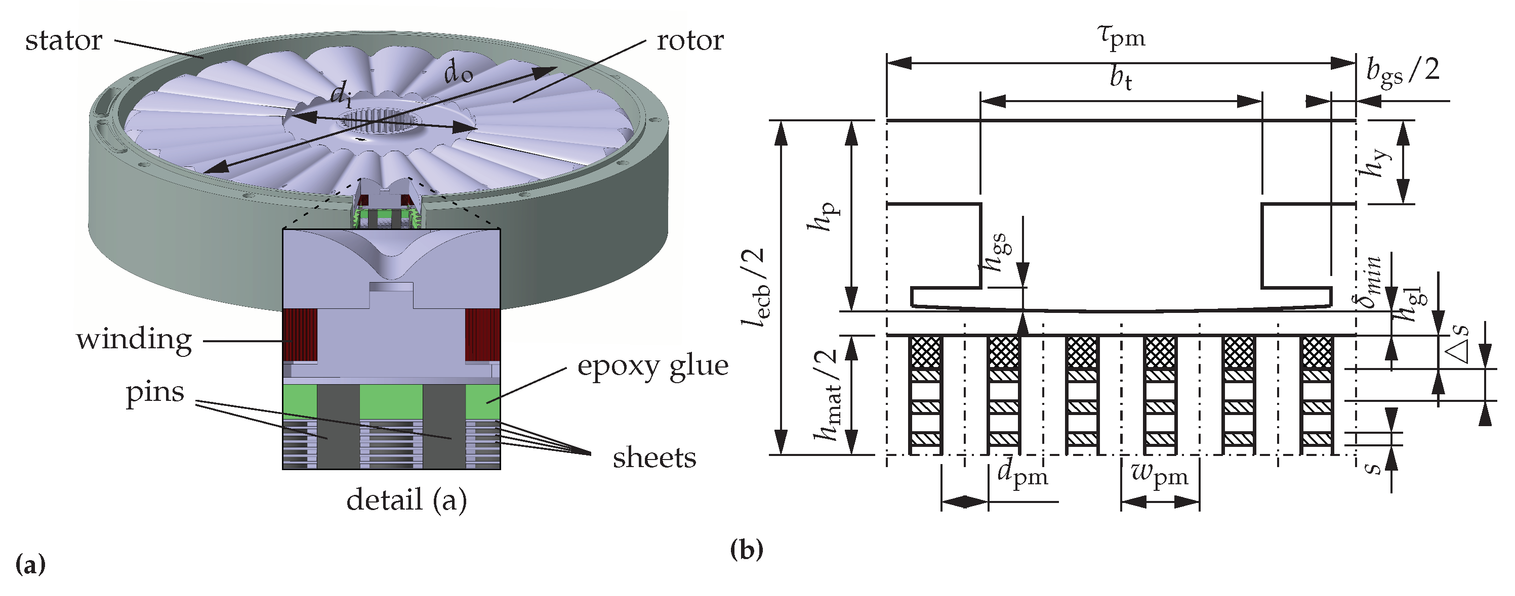
The main goal of the electromagnetic model is to determine the induced eddy currents and the resulting wear-free torque as a function of the speed n for different excitation currents $I_{\mathrm{ex}}$ and magnetic air gaps ${\delta }_{\mathsf{\mu }}$ [11]. In context of the hybrid brake, the normal force $F_{n\mu }$ also needs to be calculated with the electromagnetic model which is designed for the eddy currend brake with the magneto-isotropic material structure shown in Figure 5. The model is based on the following assumptions and simplifications:

• The model is a reluctance network;
• The model is a quasi static model;
• The magnetic circuit is modelled two-dimensionally in a pole cross-section at the mean effective radius in order to calculate the mean eddy current across all pin columns in the radial direction.

Because the model is quasi stationary, only the average torque $\overline{M}$ over one revolution at a constant angular speed $\omega$, constant excitation current $I_{\mathrm{ex}}$, and constant temperature of an ECB can be determined from the energy balance of the ECB, including the mechanical power $\overline{M}\omega$, the average ohmic losses $P_{\mathrm{ec}}$ in the active material as a result of the eddy currents $I_{\mathrm{ec}}$, the average hysteresis losses $P_{hyst}$, and the mechanical friction losses $P_{fric}$. The hysteresis losses are only taken into account in the pins and mixed with eddy current losses in the pins to compute the pin iron losses $P_{\mathrm{iron}}$.

Figure 6 shows the reluctance network with $N_{\tau m}$ pins in one pole pitch ${\tau }_{\mathrm{pm}}$. The excitation current $I_{ex}$ and the eddy currents $i_{i,j}$ in the material structure cause a magnetic flux ${\varphi }_{i,j}$ in each pin segment, where i is the pin index in the tangential (movement) direction, and j is the index of the pin segment with the length $\Delta s$ (see right side in Figure 5b) in the axial direction.

The reluctance network results in the mesh equation

$$\begin{array}{c}\hfill \left(\sum R_{\mathrm{ijn}}\right){\varphi }_{\mathrm{m}i,j}-\sum \left({\varphi }_{\mathrm{m}ijn}{R}_{\mathrm{i},\mathrm{j},\mathrm{n}}\right)=-{\displaystyle \frac{{\varphi }_{\mathrm{m}(i+1,j)}-{\varphi }_{\mathrm{m}(i-1,j)}}{R_{\mathrm{e}}2w_{\mathrm{pm}}}}v+I_{\mathrm{ex}}\end{array}$$

(8)

where ${\varphi }_{\mathrm{m}ij}$ is mesh flux of the mesh $ij$, which is analogous to the vector potential A in the transient magnetic field diffusion equation [16]. Further, $R_{ijn}$ are the path reluctances of one mesh $ij$ to neighboured meshes with the flux ${\varphi }_{\mathrm{m}ijn}$. Corresponding to Figure 6, the sum of the reluctances in the first term is

$$\begin{array}{c}\hfill \sum R_{\mathrm{ijn}}=R_{\mathrm{t}i,j}+R_{\mathrm{t}i,j+1}+R_{\mathrm{a}i,j}+R_{\mathrm{a}i+1,j}\end{array}$$

(9)

$R_{\mathrm{e}}$ is the electric resistance of one eddy current path, and $I_{\mathrm{ex}}$ is the external applied excitation current, which only exists in the meshes with excitation windings. The first term on the right represents the eddy currents $j_{ij}$ as a result of the mesh flux change and is the outcome of applying the chain rule to the flux change over time due to the speed of the rotor v at the mean effective radius and the discretisation by the central difference, where $w_{\mathrm{pm}}$ is the distance between two adjacent pins in the direction of movement.

$$\begin{array}{c}\hfill {\displaystyle \frac{\partial {\varphi }_{\mathrm{m}}}{\partial t}}={\displaystyle \frac{\partial {\varphi }_{\mathrm{m}}}{\partial x}}{\displaystyle \frac{\partial x}{\partial t}}={\displaystyle \frac{\partial {\varphi }_{\mathrm{m}}}{\partial x}}v\approx {\displaystyle \frac{{\varphi }_{\mathrm{m}i+1,j}-{\varphi }_{\mathrm{m}i-1,j}}{2w_{\mathrm{pm}}}}v\end{array}$$

(10)

To transform Equation (8) into a system of equations that can be solved numerically, the first term on the right side is moved to the left, and some entries of the resulting system matrix contain $v/\left(R_{\mathrm{e}}2w_{\mathrm{pm}}\right)$. This equation system, with the solution vector containing the mesh fluxes, is solved iteratively considering the nonlinear magnetisation curve of the excitation system as well of the steel pins in the magnetoisotropic material structure which, in this case, is also a function of the frequency $f=pn$. The average power in joules over one revolution as a result of the eddy currents is computed from the resulting mesh fluxes ${\varphi }_{\mathrm{m}(i,j)}$ with

$$\begin{array}{cc}{\overline{P}}_{\mathrm{ec}}\hfill & =\left[\sum _{j=1}^{j=2\lfloor N_{\mathrm{sh}}/2\rfloor }\sum _{i=1}^{i=N_{\mathrm{p}\tau }}{\left({\displaystyle \frac{{\varphi }_{\mathrm{m}(i+1,j)}-{\varphi }_{\mathrm{m}(i-1,j)}}{\sqrt{R_{\mathrm{e}}}2w_{\mathrm{pm}}}}v\right)}^2\right]+\hfill \\ \hfill & +\sum _{i=1}^{i=N_{\mathrm{p}}\tau }{\left({\displaystyle \frac{{\varphi }_{\mathrm{m}(i+1,j=\lceil N_{\mathrm{sh}}/2\rceil )}-{\varphi }_{\mathrm{m}(i-1,j=\lceil N_{\mathrm{sh}}/2\rceil )}}{\sqrt{R_{\mathrm{e}}}2w_{\mathrm{pm}}}}v\right)}^2\left({\displaystyle \frac{1-{(-1)}^{N_{\mathrm{sh}}}}{2}}\right)\hfill \end{array}$$

(11)

The floor function $\lfloor N_{\mathrm{sh}}/2\rfloor$ and second term of this equation consider the symmetry boundary condition in the axial direction if the number of sheets $N_{\mathrm{sh}}$ is a odd number. Due to the antisymmetric boundary conditions for $i=1$, the mesh flux is

$$\begin{array}{c}\hfill {\varphi }_{\mathrm{m}(i-1,j)}=-{\varphi }_{\mathrm{m}(i=N_{\mathrm{p}\tau },j)}\end{array}$$

(12)

and for $i=N_{\mathrm{p}\tau }$

$$\begin{array}{c}\hfill {\varphi }_{\mathrm{m}(i+1,j)}=-{\varphi }_{\mathrm{m}(i=1,j).}\end{array}$$

(13)

From the energy balance of the eddy current brake, the average torque over one revolution is calculated with

$$\begin{array}{c}\hfill {\overline{M}}_{\mathrm{ec}}={\displaystyle \frac{{\overline{P}}_{\mathrm{ec}}+{\overline{P}}_{\mathrm{iron}}}{2\pi n}}\end{array}$$

(14)

The magnetic attraction force between the rotor and stator is calculated with a co-energy approach [12,13,14]. At a constant excitation current $I_{\mathrm{ex}}$ and constant speed n, the magnetic attraction force is determined with the derivative of the co-energy $W_{\mathrm{c}}$ with respect to the magnetic air gap ${\delta }_{\mu }$.

$$\begin{array}{c}\hfill F_{\mathrm{n}\mu }={\displaystyle \frac{\partial W_{\mathrm{c}}(I_{\mathrm{ex}},n,{\delta }_{\mu })}{\partial {\delta }_{\mu }}}\end{array}$$

(15)

The total co-energy is the sum of the co-energy of every domain that is penetrated by a magnetic flux. For the flux path’s trough air, the co-energy is simply

$$\begin{array}{c}\hfill W_{\mathrm{c}}={\displaystyle \frac{{\varphi }^2}{2}}{R}_{\mathrm{m}},\end{array}$$

(16)

where $\varphi$ is the magnetic flux penetrating the flux path which has the reluctance $R_{\mathrm{m}}$. In flux paths with nonlinear magnetisation curves, the co-energy is computed from the material’s specific co-energy as a function of the flux density and the volume of the flux path.

In the system model (see Figure 4b), the electromagnetic model contains lookup tables with precomputed values for the eddy current torque $M_{\mathrm{ec}}$ and the magnetic attraction force $F_{n\mu }$ as a function of the excitation current $I_{\mathrm{ex}}$, the magnetic air gap ${\delta }_{\mu }$, and the speed n. Figure 7 shows the eddy current torque $M_{\mathrm{ec}}$ and the normal force $F_{\mathrm{n}\mu }$ as a function of the magnetic air gap ${\delta }_{\mu }$ and the excitation current $I_{\mathrm{ex}}$ for speeds of n = 1000 min⁻¹ and n = 8000 min⁻¹.

6. Spring Model

The main task for the spring is to decrease the normal force such that the wear reduction is as high as possible under the requirement that the brake torque can be generated. Additionally, the spring provides a reset of the axial rotor position and transfers the torque from the rotor to the shaft. The first approach to the spring is to design it as a wave spring. The spring lies against a tangential contour during compression, as shown in Figure 8a. Due to the limited design space, the mean spring diameter $d_{\mathrm{ms}}$, the width $b_{\mathrm{s}}$, and the total height of the spring $h_{\mathrm{stot}}$ are given. The parameters to be optimized are the spring wavenumber $N_{\mathrm{sw}}$, the thickness of a spring leaf $h_{\mathrm{ssh}}$, and the contour radius $r_{\mathrm{c}}$.

The model is based on the Euler–Bernoulli beam theory with the governing equation for the deflection w along the path x

$$\begin{array}{c}\hfill EI{\displaystyle \frac{{\mathrm{d}}^{4}w}{\mathrm{d}{x}^4}}=q\end{array}$$

(17)

where E is the Young’s modulus, I is the second moment of the area, and q is the specific surface load, which is zero in this case. Due to symmetry, a spring leaf is divided over $4N_{\mathrm{sw}}$ quarter sections of length

$$\begin{array}{c}\hfill L_{\mathrm{qs}}={\displaystyle \frac{\pi (d_{\mathrm{os}}+d_{\mathrm{is}})}{8N_{\mathrm{sw}}}}\end{array}$$

(18)

as shown in Figure 8b. Further, the model is related to the middle spring sheet. When the spring comes into contact with the contour, the bending moment remains constant up to the end point of the contact due to the radius of curvature $r_{\mathrm{c}}+h_{\mathrm{stot}}/2$.

$$\begin{array}{c}\hfill M_{\mathrm{et}}={\displaystyle \frac{EI}{r_{\mathrm{c}}+{\displaystyle \frac{h_{\mathrm{stot}}}{2}}}}\end{array}$$

(19)

If the force F is given, the point at which the contact ends can be determined with

$$\begin{array}{c}\hfill x_{\mathrm{ec}}=L_{\mathrm{qs}}-{\displaystyle \frac{M_{\mathrm{et}}2N_{\mathrm{sw}}{N}_{\mathrm{s}}}{F}}\end{array}$$

(20)

Due to the strong deflection along the contour, the deflection of the free beam length is calculated in a separate coordinate system that is rotated by the angle

$$\begin{array}{c}\hfill \phi =arcsin\left({\displaystyle \frac{x_{\mathrm{ec}}}{r_{\mathrm{c}}+{\displaystyle \frac{h_{\mathrm{stot}}}{2}}}}\right)\end{array}$$

(21)

and shifted by the vector

$$\begin{array}{c}\hfill x_{\mathrm{ec}};\hspace{1em}{y}_{\mathrm{et}}=\sqrt{{\left(r_{\mathrm{c}}+{\displaystyle \frac{h_{\mathrm{stot}}}{2}}\right)}^2-x_{\mathrm{et}}^2}-r_{\mathrm{c}}\end{array}$$

(22)

with respect to the main coordinate system. The force F acts with its component

$$\begin{array}{c}\hfill F_{\mathrm{fy}}=Fcos\left(\phi \right)\end{array}$$

(23)

in the coordinate system on a free bar of length

$$\begin{array}{c}\hfill L_{\mathrm{f}}=L_{\mathrm{qs}}-\phi r_{\mathrm{c}}\end{array}$$

(24)

and leads to a free deflection of

$$\begin{array}{c}\hfill s_{\mathrm{fy}}={\displaystyle \frac{F_{\mathrm{fy}}{L}_{\mathrm{f}}^3}{3EI2N_{\mathrm{sw}}{N}_{\mathrm{s}}}}\end{array}$$

(25)

The reverse transformation to the main coordinate system then leads to the deflection of the spring

$$\begin{array}{c}\hfill s=2\{s_{\mathrm{sy}}cos\left(\phi \right)+r_{\mathrm{c}}(1-cos\left(\phi \right))+L_{\mathrm{f}}sin\left(\phi \right)\}\end{array}$$

(26)

7. Spring Parameter Analysis

After a transient simulation of the system model, the quality criteria are evaluated by varying the spring parameters, each of which leads to different spring characteristics. Figure 9 shows different design points in the space of the quality criteria.

For a better understanding of the system, the behaviour is analysed in detail for three different design points. The red, green, and blue design points (design 1–3) are each a result of spring parameters that produce the spring characteristics shown in Figure 10.

Each of these spring characteristics results in a different dynamic behaviour, illustrated by the state trajectories in Figure 11. It is evident that design 2, with the green spring curve, results in the lowest time to rotor contact with the stator and the highest impact velocity, because it has the lowest stiffness and preload. Design 1, with the red spring curve, gives the highest time to impact, a very low impact velocity, but also, a dynamic behaviour with a high number of periodic oscillations (see Figure 11). At some point, the spring force exceeds the magnetic attraction force, slowing the axial motion of the rotor and causing it to move back. Design 3 offers a tradeoff between a lower time to impact and a lower oscillation rate. In Figure 12, it is clear that designs that result in a higher time to contact also have a higher wear reduction factor, because the frictional torque stays at zero longer. 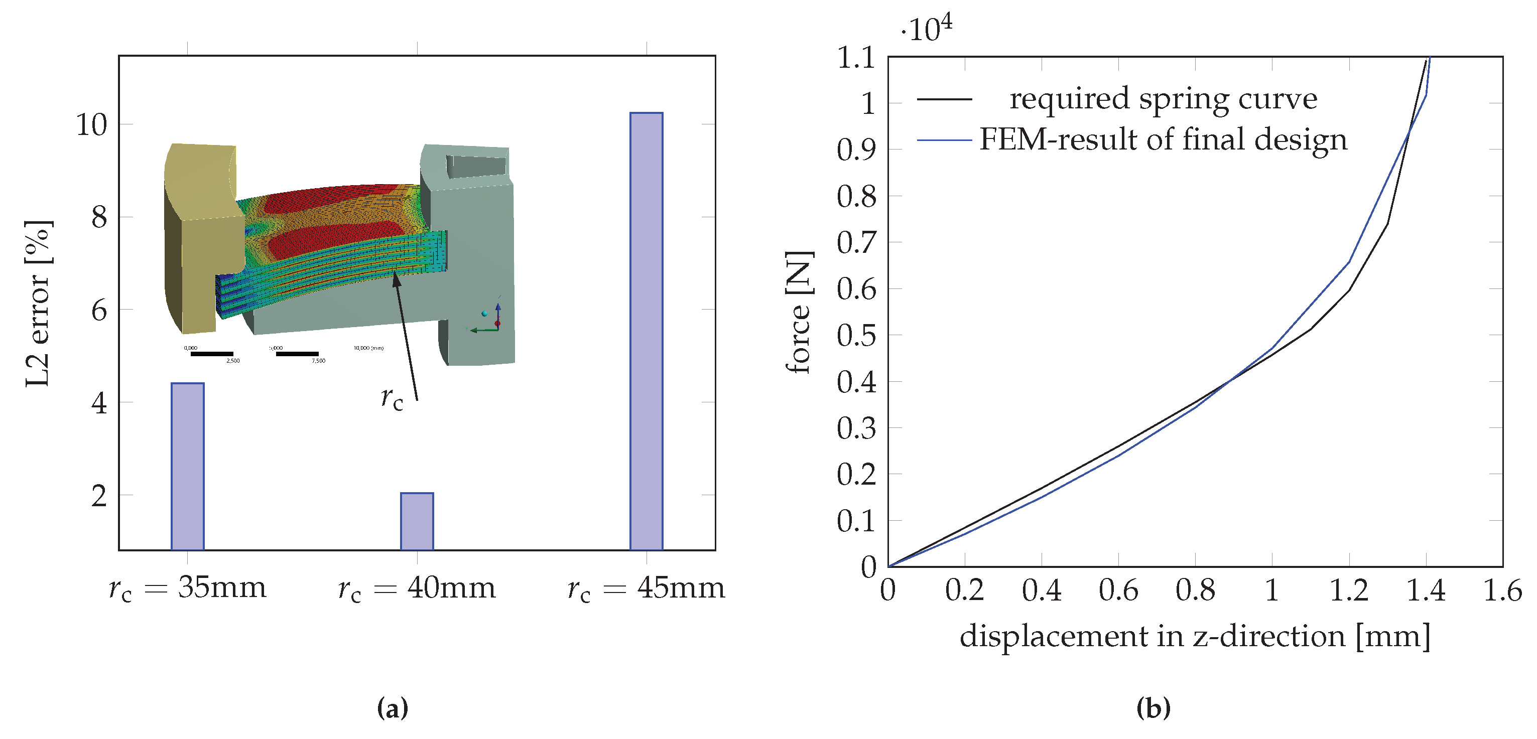Design 1 has the highest wear reduction factor of $\Delta {\epsilon }_{\mathrm{w}}=0.9$, but also results in torque oscillations due to the unstable motion of the rotor. Design 3 is the design with the next highest wear reduction factor of $\Delta {\epsilon }_{\mathrm{w}}=0.85$ and an acceptable aperiodic factor of ${\gamma }_{\mathrm{ap}}=0.8$. This design, which yields the blue spring curve, will be selected to build a functional demonstrator for future experiments. To ensure that the spring design will result in the desired spring curve in reality, an finite element method (FEM) analysis is performed.

8. FEM Analyses

During the design process, it was determined that the tangential contour spring mechanism would most likely be difficult to manufacture. The final design is axisymmetric, and therefore, much easier to manufacture. It consists of a diaphragm spring that can contact a radial contour of the hub. This design was not initially considered because it was thought that such a design would have excessive mechanical stress for the required forces for the given installation space. The stresses are high, with a value of σ = 1200 N mm⁻², but a spring steel with a tensile strength of σ_all = 1800 N mm⁻² is used. In order to achieve the desired spring characteristics, even with the modified design, a parameter study was performed using the FEM model. Figure 13a shows an example of the relative mean square deviation of the spring characteristic from the required one, which was obtained for different contour radii $r_{\mathrm{c}}$. Figure 13b shows the spring characteristic curve of the final spring design calculated with the FEM. The relative mean square error of this spring curve is less than 3% compared to the desired one.

9. Experimental Setup and Methods

The aim of the experiment was to demonstrate the operating principle and generate data to validate the system model. Primarily, the torque M was measured at constant speeds n for different excitation currents $I_{\mathrm{ex}}$ on a dynamometer test bench. In detail, the electromagnetic and mechanical behaviours were analysed with additional measurement techniques.

9.1. Measurement Setup

Figure 14 shows a simplified CAD model of the function demonstrator with the parameters given in

Table 1. Parameters of the functional demonstrator corresponding to Figure 4b and Figure 5a,b.

Parameter	Symbol	Value	Unit
outer active diameter	$d_{\mathrm{o}}$	$0.25$	$\mathrm{m}$
active length	$l_{\mathrm{ecb}}$	$0.05$	$\mathrm{m}$
active length one rotor	$l_{\mathrm{r}}$	$0.0167$	$\mathrm{m}$
active length stator	$l_{\mathrm{s}}$	$0.02$	$\mathrm{m}$
maximum magnetic air gap	${\delta }_{\mu \max }$	$0.0013$	$\mathrm{m}$
maximum mechanical air gap	${\delta }_{\max }$	$0.0007$	$\mathrm{m}$
predeformation	$s_0$	$0.00065$	$\mathrm{m}$

. The maximum mechanical air gap ${\delta }_{\max }$ and the predeformation of the spring $s_0$ are shown in Figure 4b. The entire measurement setup on a dynamometer test bench is shown in Figure 15. To validate the electromagnetic model, the excitation current $I_{\mathrm{ex}}$ and the magnetic flux in the pole core and material structure were measured. The excitation current was measured by the DC power supply itself, and the analogous measured value was transmitted to the DAQ system. For correct validation of the electromagnetic model, it was necessary to measure the temperatures of the cooling fluid ${\vartheta }_{\mathrm{in}}$ and ${\vartheta }_{\mathrm{out}}$ to estimate the temperatures of the sheets inside the material structure (see Figure 5b) with the heat transfer model of [17]. To distinguish between the torque generated by eddy currents and the frictional torque, the frictional torque was measured separately. For this purpose, the brake pads were mounted on force sensors. These force sensors were bending beam sensors with strain gauges.

To measure the magnetic flux in the material structure, seven flux probes were attached to three flux guide elements (pins) in the material structure. Figure 16a shows the positions of the flux probes in the material structure, and Figure 16 shows a flux probe on a flux guiding element. The flux was measured by the induced voltage in the probes with a power analyser. By integrating the measured voltage over time and dividing by the number of turns in the probes, the magnetic flux was determined in a postprocessing step.

Since the magnetic flux and thus the eddy currents and the rotor position depend on the magnetic air gap, ${\delta }_{\mu }$ was measured with three laser distance sensors, as shown in Figure 17. Since the fit of the linear guide was not perfect, a postprocessing step with three laser sensors determined the angle ${\gamma }_{\mathrm{r}}$ and thus the spatial position of the rotor and the air gap as a function of the fixed $r-\phi$ coordinates of the stator and time.

9.2. Measurement of Friction Torque

To distinguish between the torque due to eddy currents and the mechanical frictional torque, the frictional force on the brake pads was measured using the force sensors shown in Figure 14. Figure 18 shows the resulting force signal for a speed of n = 1000 min⁻¹ and an excitation current of I_ex = 50 A. It can be seen that the signal was most likely disturbed by temperature effects.

To obtain more accurate measurement results, an alternative method must be found to distinguish between torques. One idea is to calculate the torque as a result of the eddy currents $M_{\mathrm{ec}}$ from the measured magnetic flux in the pins by using a simplified version of Equation (11) in Equation (14). The torque calculated from the measured fluxes is calculated using

$$\begin{array}{cc}\hfill {\overline{M}}_{\mathrm{ecmeas}}& ={\displaystyle \frac{C_{\mathrm{measT}}n}{{\rho }_{20}\left[1+{\alpha }_{\mathrm{el}}\left({\vartheta }_{\mathrm{sh}}-{20}^{\circ }\mathrm{C}\right)\right]}}\sum _{i=1}^{i=N_{\tau }}[{\left({\varphi }_{\mathrm{fp}6(i+1)}-{\varphi }_{\mathrm{fp}6(i-1)}\right)}^2+\hfill \\ \hfill & {\left({\varphi }_{\mathrm{fp}4(i+1)}-{\varphi }_{\mathrm{fp}4(i-1)}\right)}^2+{\left({\varphi }_{\mathrm{fp}2(i+1)}-{\varphi }_{\mathrm{fp}2(i-1)}\right)}^2]\hfill \end{array}$$

(27)

where ${\varphi }_{\mathrm{fp}2}$, ${\varphi }_{\mathrm{fp}4}$ and ${\varphi }_{\mathrm{fp}6}$ are the measured fluxes in the pins measured with the field coils shown in Figure 16, $N_{\tau }$ is the number of equidistant data points under a pair of poles, and $C_{\mathrm{measT}}$ is a constant. The constant $C_{\mathrm{measT}}$ with units of $\mathrm{m}$ is determined with a measured torque and fluxes of a measurement where no contact occurs between the rotor and stator, and the total measured torque is the torque as a result of eddy currents and iron losses. The temperature of the plates ${\vartheta }_{\mathrm{sh}}$ is approximated with the measured power and the inlet and outlet temperatures of the cooling water (see Figure 15) using the Nusselt correlation in [17]. To test this method, a measurement was made with the spring mechanism locked and a magnetic air gap of ${\delta }_{\mu }=1.3$ mm, so that all measured torques were the result of eddy currents and could, in principle, be calculated using Equation (27). Figure 19 shows the measured torques and the torques calculated with the measured flux in the material structure at different speeds and excitation currents. Up to a speed of n = 6500 min⁻¹, the error between the torque calculated with the measured magnetic fluxes and the directly measured torque was less than 10%. The large difference at speeds above n = 6500 min⁻¹ was most likely due to deformation of the rotor due to centrifugal forces (see discussion).

10. Results

10.1. Stationary Electromagnetic Validation

The first step of validation was to compare the calculated primary magnetic field with the experimental measurements. Figure 20a shows the predicted and measured flux density in the pole core (see Figure 16b) for different excitation currents at a constant air gap of ${\delta }_{\mu }=0.5$ mm and the error between measurement and prediction. In addition, the validity was evaluated with respect to the steady-state field at a constant current for different air gaps. Figure 20b shows the measured and predicted flux densities in the pole core and in the centre steel pin, measured with flux probe 6 (see Figure 16), and the error between the measurement and prediction. It can be seen that the maximum error between the prediction and measurement is 0.1 Tesla, which is less than 10% of the measured maximum value of 1.6 Tesla.

10.2. Stationary Validation Membrane Spring

To validate the submodel of the membrane spring, the force–displacement curve of different springs was measured on a tensile testing machine. Figure 21a shows the force–displacement curve of the spring chosen for the experiment as a result of a FEM analysis and as a result of an experiment. The dashed line shows the result of the FEM analysis where only the spring sheets are deformable to save the computing time. This FEM result differs strongly from that of the experiment over the entire range of displacement. A much better result is given by the FEM analysis where the contour bush and the shaft are implemented as deformable parts as well (see Figure 21b). Because of the deformation of the shaft nut, the spring sheet package is bent around a resulting contact point. This results in a less stiff behaviour compared to that shown in the FEM analysis with solid contour bush and shaft nut.

10.3. Measurement Results and Validation of the Overall System

The main goal of the measurement was the evaluation of wear free torque as a result of induced eddy-currents and the friction torque. Figure 22 shows the experimentally evaluated proportion of torque due to eddy currents in the space of torque and speed. It can be seen that the higher the speed, the higher the portion of wear-free eddy current torque. Because of the higher excitation current and, therefore, the higher magnetic attraction force, the mechanical portion increases with the torque at low speeds. At speeds of higher than 3500 rpm, the torque is delivered wear-free.

The validation of the overall system was performed step-by-step. First, the electromagnetic model used to calculate the torque of eddy currents was validated with the measured air gap, which means by neglecting the spring model. Figure 23 shows the relative error of the predicted to the experimentally measured eddy current torque $\Delta M_{\mathrm{err},\mathrm{ec}}$ in the space of torque and speed. Most of the data points show a relative error of lower than 10%. However, there are relatively high errors for an excitation current of $I_{\mathrm{ex}}=10$ A and $I_{\mathrm{ex}}=20$ A in the speed range of n = 4000 min⁻¹ to n = 7500 min⁻¹. Additionally, in the lower-speed region at excitation currents of $I_{\mathrm{ex}}=30$ A to $I_{\mathrm{ex}}=50$ A, there are relatively large errors. The reason for the errors in the low-torque region are most likely a result of frictional torques in the test bed. At all other measured points, it is assumed that the errors are mostly a result of the fact that the air gap is not homogenous in the radial direction, and the air gap is only measured at a radius of $r=0.1$ m when the outer radius of the poles is $r_{\mathrm{o}}=0.125$ m.

In Figure 24, the air gap over speed is shown, where the colours show the corresponding calculated normal force. At a low excitation current and, therefore, a low magnetic attraction force, the measured air gap increases at high speeds. This means that the rotor becomes deformed in the axial direction by centrifugal forces such that the air gaps are inhomogeneous in the radial direction (see discussion). Therefore, it also becomes deformed as a result of the magnetic attraction force but in the other direction. Hence, the air gap along the radius during measurement is unknown, except at the radius, where the laser distance sensors are positioned. The deformation of the rotor not only results in an unknown air gap but also strongly affects the overall system behaviour.

For a certain reduction in the air gap, a significantly lower attraction force is necessary than in theory. Figure 25 shows the magnetic attraction force calculated with the measured air gap over the measured air gap, where the black curve is the measured spring curve. Because of the predeformation of the membrane spring, which is $s_0=0.65$ mm, in theory, there should be no reduction in the air gap up to a magnetic attraction force of $F_{\mathrm{N}\mu }=3000$ N. However, because of the rotor deformation, the air gap decreases immediately with an increase in the magnetic normal force.

11. Discussion

In this work, the model and design method of a hybrid brake were presented. Finally, a working demonstrator was tested. Most importantly, the results show that it is possible to use the magnetic attraction of an eddy current brake to brake to a stop at very low speeds. The spring that enables the axial movement of the rotors was optimised for high wear reduction as well as stable dynamic behaviour. Due to the friction in the bushing, no axial vibrations were detected or measured during the tests. Therefore, it should be possible to use a spring design that leads to a higher wear reduction, which was assumed in the design process to lead to strong vibrations (see design 1 in the spring parameter analysis section). The wear reduction has not yet been analysed because the torque–speed map has not yet been fully measured. Furthermore, the measurement data show strong deformation of the rotor, so the air gap is inhomogeneous along the radius. The validation of the subsystems was successful. Both the electromagnetic model for calculating the primary magnetic flux and the FEM model of the spring deviate from the experimental results by less than 10%. The proposed method for calculating the eddy current moment from the measured magnetic fluxes was also successfully tested. The final validation of the overall system was only partially possible due to the deformation of the rotor, which resulted in an inhomogeneous air gap. Even if the air gap had been measured at more points, validation of the model would also not have been possible, because the electromagnetic model is a two-dimensional model. Therefore, the electromagnetic model must be extended to a three-dimensional model, and the laser distance sensors should be positioned at different radial locations for complete model validation. Since the material structure of the active element is probably not suitable for mass production, the magneto-isotropic material structure must be improved in terms of it’s cost-effective manufacturability.

References

1. Holtmann, C. Design and Optimization Method for a High Power Eddy Current Brake with a Magneto Isotropic Material Structure for the Use in Electrified Heavy Duty Trucks. In Proceedings of the EUROBRAKE 2021, Online, 17–21 May 2021. [Google Scholar]
2. Gay, S.E.; Ehsani, M. Optimized Design of an Integrated Eddy-Current and Friction Brake for Automotive Applications. In Proceedings of the 2005 IEEE Vehicle Power and Propulsion Conference, Chicago, IL, USA, 7–9 September 2005; IEEE: Piscataway, NJ, USA, 2005; pp. 189–193. [Google Scholar] [CrossRef]
3. Yazdanpanah, R.; Mirsalim, M. Hybrid Electromagnetic Brakes: Design and Performance Evaluation. IEEE Trans. Energy Convers. 2015, 30, 60–69. [Google Scholar] [CrossRef]
4. Huang, S.; Bao, J.; Ge, S.; Yin, Y.; Liu, T. Design of a frictional–electromagnetic compound disk brake for automotives. Proc. Inst. Mech. Eng. Part J. Automob. Eng. 2020, 234, 1113–1122. [Google Scholar] [CrossRef]
5. Wang, K.; He, R.; Tang, J.; Liu, R. Design and thermal analysis of a novel permanent magnet-friction integrated brake for vehicle. Therm. Sci. 2020, 24, 1827–1834. [Google Scholar] [CrossRef]
6. Holtmann, C. Bremsvorrichtung und Fahrzeug. DE 10 2018 212 386 B4. 25 July 2018. [Google Scholar]
7. Takeuchi, M.; Katsura, S. Robust Velocity Control for Electromagnetic Friction Brake Based on Disturbance Observer. IEEJ J. Ind. Appl. 2023. [Google Scholar] [CrossRef]
8. Bochkarev, I.V.; Khramshin, V.R.; Voronin, S.S.; Bryakin, I.V. Diagnostics of Electromagnetic Friction Brakes and Clutches. In Proceedings of the 2019 IEEE Conference of Russian Young Researchers in Electrical and Electronic Engineering (ElConRus), St. Petersburg and Moscow, Russia, 28–31 January 2019; Shaposhnikov, S.O., Ed.; IEEE: Piscataway, NJ, USA, 2019; pp. 447–452. [Google Scholar] [CrossRef]
9. Holtmann, C. Eddy Current- and Friction Brake Fusion by a Disc-Spring to a Hybrid- Brake. In Proceedings of the 2021 24th International Conference on Mechatronics Technology (ICMT), Singapore, 18–22 December 2021; IEEE: Piscataway, NJ, USA, 2021; pp. 1–6. [Google Scholar] [CrossRef]
10. von Glasner, E.C. Bremssysteme und Bremsverhalten von Nutzfahrzeugen und Zügen. In Bremsenhandbuch; Springer: Berlin/Heidelberg, Germany, 2012; pp. 165–197. [Google Scholar]
11. Holtmann, C.; Mockel, A. 2D Reluctance Model of an Eddy Current Brake with a Magneto Isotropic Material Structure. In Proceedings of the 2020 International Conference on Electrical Machines (ICEM), Gothenburg, Sweden, 23–26 August 2020; IEEE: Piscataway, NJ, USA, 2020; pp. 578–584. [Google Scholar] [CrossRef]
12. Mawardi, O.B. On the concept of coenergy. J. Frankl. Inst. 1957, 264, 313–332. [Google Scholar] [CrossRef]
13. Jeltsema, D.; Scherpen, J.M.A. Multidomain modeling of nonlinear networks and systems. IEEE Control. Syst. Mag. 2009, 29, 28–59. [Google Scholar]
14. Hadžiselimović, M.; Virtič, P.; Štumberger, G.; Marčič, T.; Štumberger, B. Determining force characteristics of an electromagnetic brake using co-energy. J. Magn. Magn. Mater. 2008, 320, e556–e561. [Google Scholar] [CrossRef]
15. Coblaş, D.; Broboana, D.; Balan, C.; Hejjam, M. Numerical Simulation of Constant Velocity Squeeze Flow. U.P.B. Sci. Bull. Ser. D 2013, 75, 165–174. [Google Scholar]
16. Mladen, Z. Theory and Numerical Modelling of Lorentz Force Eddy Current Testing. Ph.D. Thesis, TU Ilmenau, Ilmenau, Germany, 2013. [Google Scholar]
17. Kohler, C.; Holtmann, C.; Rinderknecht, F.; Arens, L. Experimental Examination of the Heat Transfer in a High Power Eddy Current Brake with a Magneto-isotropic Material Structure. In Proceedings of the 2022 Second International Conference on Sustainable Mobility Applications, Renewables and Technology (SMART), Cassino, Italy, 23–25 November 2022; IEEE: Piscataway, NJ, USA, 2022; pp. 1–7. [Google Scholar] [CrossRef]
Figure 1. Theoretical torques of an eddy current brake with a linearly decreasing speed over time and a friction brake for low speeds.
Electronics 12 02632 g001
Figure 2. Exemplary CAD model of a hybrid brake (a) and superordinate operating principle of the hybrid brake (b).
Electronics 12 02632 g002
Figure 3. Torques over time for the use of a membrane spring with zero stiffness.
Electronics 12 02632 g003
Figure 4. System model of the hybrid brake (a) and mechanical domain of the model (b).
Electronics 12 02632 g004
Figure 5. CAD model of the rotational axial flux ECB, where detail a shows one half pole cross-section in the tangential–axial plane at the middle effective radius corresponding to Figure 5b (a) and the geometrical parameters of one pole cross-section (b).
Electronics 12 02632 g005
Figure 6. Two-dimensional reluctance network. Air reluctances are presented in white, steel reluctances are grey, and air gap reluctances are light grey because they include the pin reluctances next to the air gap corresponding to h gl in Figure 5b.
Electronics 12 02632 g006
Figure 7. Eddy current torque M ec (a) and magnetic normal force F n μ (b) as a function of the air gap and excitation current for different speeds (n = 1000 min−1 and n = 8000 min−1).
Electronics 12 02632 g007
Figure 8. Schematic three-dimensional geometry of the spring mechanism with a nondeflected spring with a spring wavenumber of N sw = 6 (a). Quarter geometry of the middle with the force F deformed and a spring sheet with the limiting contour (b).
Electronics 12 02632 g008
Figure 9. Results of the spring parameter analyses. t con : time until contact, v imp : impact velocity, γ ap : aperiodic factor. The coloured points (designs 1 to 3) are related to the spring curves in Figure 10 and the state space trajectories in Figure 11.
Electronics 12 02632 g009
Figure 10. Spring curves for spring parameters resulting in the quality criteria marked with the red, green, and blue points in Figure 9 and the corresponding time-dependent magnetic normal forces projected in the spring curve plane.
Electronics 12 02632 g010
Figure 11. State space trajectories for the axial movement of the rotor for different spring parameters resulting in different impact velocities, times to impact, and aperiodic factors.
Electronics 12 02632 g011
Figure 12. Torques over time for the spring designs with the spring curves shown in Figure 10.
Electronics 12 02632 g012
Figure 13. Optimisation of the contour of the spring mechanism in the FEM (a) and the desired spring curve vs. the final spring curve as a result of the FEM calculation (b).
Electronics 12 02632 g013
Figure 14. Simplified CAD model of the functional demonstrator.
Electronics 12 02632 g014
Figure 15. Measurement setup on the dynamometer test bed.
Electronics 12 02632 g015
Figure 16. Positions of the flux probes (fp) in the material structure (a) flux probes at the pole core and pole plate (b).
Electronics 12 02632 g016
Figure 17. Positions of the laser distance sensors (a) and the laser distance sensors at the hybrid brake (b).
Electronics 12 02632 g017
Figure 18. Signal of the measured friction force and excitation current over time.
Electronics 12 02632 g018
Figure 19. Measured torques and torques calculated with the measured flux in the material structure at different speeds and excitation currents.
Electronics 12 02632 g019
Figure 20. Measured and predicted flux densities in the pole core B pc at δ μ = 0.5   mm for different excitation currents (a) and the measured and predicted flux densities in the pole core and in the steel pins at I ex = 90   A for different air gaps (b).
Electronics 12 02632 g020
Figure 21. Force–displacement curves of the membrane spring as a result of the FEM analysis and experiment (a) and deformed spring mechanism as a result of a FEM analysis (b).
Electronics 12 02632 g021
Figure 22. Map of the experimentally evaluated proportion of torque due to eddy currents in the space of torque and speed.
Electronics 12 02632 g022
Figure 23. Map of the relative errors in the predicted and experimentally evaluated torques due to eddy currents in the space of torque and speed for different excitation currents.
Electronics 12 02632 g023
Figure 24. Map of the simulated normal force with the measured magnetic air gap and speed for different excitation currents.
Electronics 12 02632 g024
Figure 25. Simulated normal force with the measured magnetic air gap and speed.
Electronics 12 02632 g025