Critic-Only Learning Based Tracking Control for Uncertain Nonlinear Systems with Prescribed Performance

Abstract

A critic-only learning-based tracking control with prescribed performance was proposed for a class of uncertain nonlinear systems. Based on an estimator and an optimal controller, a novel controller was designed to make tracking errors uniformly ultimately bounded and limited in a prescribed region. First, an unknown system dynamic estimator was employed online to approximate the uncertainty with an invariant manifold. Subsequently, by running a novel cost function, an optimal controller was derived by online learning with a critic-only neural network, which ensured that tracking errors can evolve within a prescribed area while minimizing the cost function. Specifically, weight update can be driven by weight estimation error, avoiding introducing an actor-critic architecture with a complicated law. At last, the stability of a closed-loop system was analyzed by Lyapunov theorem, and tracking errors evolved within prescribed performance with the optimal controller. The effectiveness of the proposed control can be demonstrated by two examples.

1. Introduction

Nowadays, many plants in the real word can be formulated as uncertain nonlinear systems, such as autonomous underwater vehicles [1], mobile robots [2], and quadrotors [3]. Thus, tracking problems for uncertain nonlinear systems have become one of the issues, and various control methods have been developed and employed in many physical systems to achieve tracking performance.

To deal with the impact induced by uncertainties during controller design, there emerge a large amount of tools to approximate uncertainties and combined with other controllers, e.g., neural networks (NNs) [4,5], fuzzy logic systems [6,7,8], and disturbance observers [9,10,11]. For example, by integrating with a backstepping control, an adaptive tracking controller is designed in [5] for uncertain nonlinear systems, where an NN is utilized to estimate the uncertain term of the model. Due to an uncertain dynamical model in surface vessels, proportional derivative feedback combined with a fuzzy logic system is proposed in [7] with satisfying tracking performance and theoretical results. Taking the disturbance ability of an observer-based controller into consideration, the tracking performance can be guaranteed. For manipulators, a sliding-mode controller is investigated for tracking problems, where a nonlinear disturbance observer is implemented to predict and remove the effect of disturbance [10]. However, manually tunned parameters limit above controllers applied in practical applications. Recently, the unknown system dynamics estimator (USDE) is a novel estimation method to deal with uncertainty and disturbance of nonlinear systems [12], where the state can be an added filtered operation such that invariant manifold is conducted for accurate estimation. Different from NNs and fuzzy logic systems with repeated tuning, the estimator only uses the system state and the control input and can achieve rapid convergence of disturbance estimation by adjusting a parameter. For the motion control of robot systems, lumped disturbances are estimated through an improved unknown disturbance estimator [13]. In [14], by implementing a USDE to compensate the disturbance, a sliding-mode control is designed to obtain the performance with fast convergence and strong robustness. Since USDEs in the above literature are aimed at integral series systems, it is difficult to solve the strong coupling and multivariable functions of nonlinear systems. Moreover, it is worth mentioning that the above control methods with an inherent structure do not discuss the output constraints such as the convergence rate and the maximum steady-state error, which are important in engineering.

Combined with reinforcement learning (RL), which is a branch of machine learning, a mass of adaptive controllers for stability of closed-loop systems have been developed. By integrating it with dynamic programming, there emerge an optimal controller with a learning ability and the balancing between the tracking performance and the control cost, which are generalized as adaptive dynamic programming (ADP) without dimensionality. One of prevalent structures is actor-critic ADP to pursue the optimal control and the optimal value function [15,16,17]. However, tracking error may satisfy the preassigned convergence in practical engineering applications. To address this issue, the introduction of the RL algorithm into the prescribed performance control (PPC) has attracted attention [18], which significantly reduces tracking error and control input and improves performance [19,20,21]. In [19], a data-driven RL algorithm for performance specification was proposed to simultaneously pursue control methods for satisfying optimality and tracking errors to meet output constraints. Combined with the fault-tolerant control (FTC), nonlinear systems with output constraints are considered by RL algorithms [22,23,24]. It is noted that it is difficult to achieve the fault tolerant control by RL alone. In [23], for nonlinear systems with actuator faults, a model-free adaptive optimal control method with specified performance was designed, where an adaptive observer is employed to estimate faults, and the incremental system parameters are estimated by the recursive least squares identification method. By combining the PPC with ADP, the optimal control strategy is obtained, such that tracking error satisfies the specified performance. By introducing an intermediate controller, a controller, and a fault tolerant controller based on RL algorithms, a fault-tolerant dynamic surface control algorithm based on actor-critic ADP was proposed in [24] for nonlinear systems with unknown parameters and actuator faults, which avoids the difficulty of RL in fault tolerant control. For the manipulator, a robust motion control method with specified performance based on reinforcement learning was proposed in [25]. The measurement noise is eliminated by carefully adding an integral term and adopting a robust generalized proportional integral observer, and an optimal control strategy based on error transformation was designed with the actor-critic ADP method to ensure the stability of the system. For the high-order nonlinear multi-agent system containing uncertainty, the optimal consistency control problem with specified performance is considered in [26], where the stability of a closed-loop system and the convergence of consensus errors within a certain range are proved. Based on an actor-critic network, the optimal control is investigated for robot [27] and pure feedback system [28] separately. It is noted that the above controllers rely on multiple neural networks to ensure the stability and optimality of the system. The weight of the neural network is complicated due to the increasing number of nodes, and many parameters are difficult to adjust. In order to satisfy the optimal predetermined performance, the main idea is to transform the constrained tracking error into an unconstrained variable by constructing transformation function, and approximate optimal control is designed within actor-actor NN by minimizing the value function related to the unconstrained variable. Noting that the Hamilton-Jacobi-Isaacs (HJI) equation can be solved for deriving the optimal control in [29,30], it is deemed to be conservative for the worst case of disturbance with massive control inputs. Moreover, existing design and theoretical analysis of the preset performance optimal control are mostly combined with fault-tolerant control, robust control, and adaptive control. There is no relevant research for the USDE-based optimal control to assure the preassigned convergence rate.

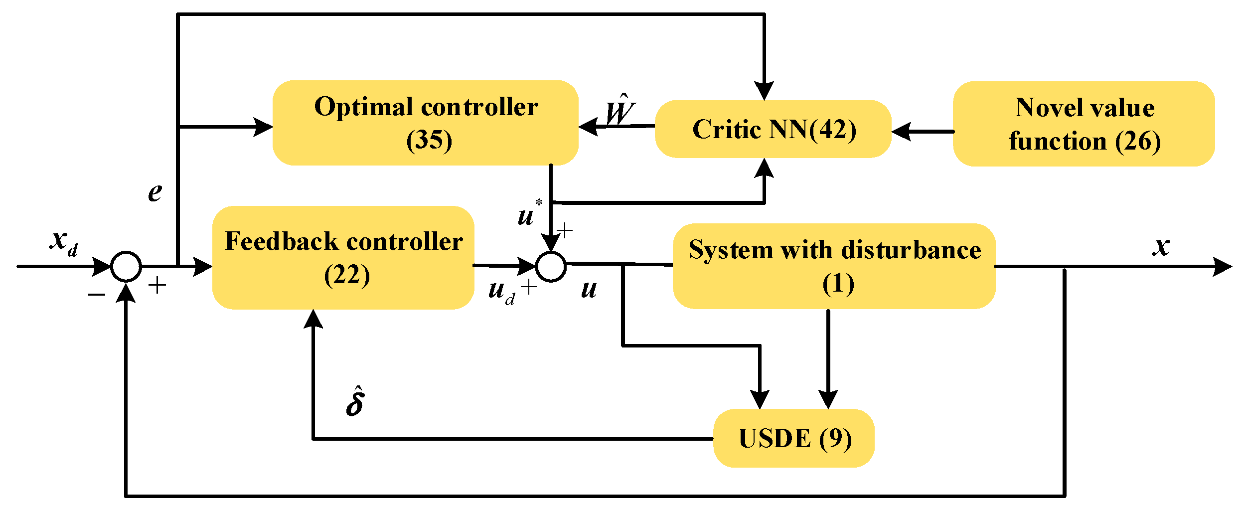
Motivated by the above statements, we proposed an optimal control with asymmetric performance constraints under the framework of critic-only ADP by constructing a new value function. The highlights in this article can be expressed as follows:

(1) Compared with the existing observer-based controllers [9,10,11], where the disturbance is estimated with observers by adjusting manually multiple parameters, the USDE was employed to approximate the lumped disturbance of nonlinear uncertain systems with an invariant manifold principle. Moreover, differing from previous function approximator-based control schemes [12,13,14], by combining the RL technique into the optimal control design, the precise tracking performance and the low control cost can be achieved.

(2) Different from the optimal control derived by the actor-critic ADP framework in [24,26,27,28], a critic-only NN was designed for online learn optimal control without constructing an actor NN. In addition, to achieve the convergence rate with a preassigned region, a novel value function was minimized, such that tracking errors can evolve within the prescribed region with low control consumption. In contrast to the traditional gradient descent for weight update in actor-critic ADP, the weight law was designed ingeniously to update the weight of a critic NN, reduce the online training computation and accelerate the weight convergence.

The outline of the article is organized as follows. We first gave the definition of the optimal tracking control problem with prescribed performance in Section 2. In Section 3, the main result of the control design was discussed, in which a feedback controller and an optimal controller were proposed. The stability analysis is illustrated in Section 4. Section 5 provides the effectiveness of the proposed controller on two examples.

Throughout this paper, the vector or matrix is represented by bold fonts, which is different from the scalar. $\mathbf{0}$ represents the zero matrix and $\mathit{I}$ denotes the identity matrix. $\mathrm{d}\mathrm{i}\mathrm{a}\mathrm{g}(\mathit{x})$ is the diagonal matrix conducted with vector $\mathit{x}$. ${\lambda }_{\min }(\cdot )$ is the minimized eigenvalue of the corresponding matrix.

2. Preliminaries

The following multiple-input–multiple-output system with disturbance is considered:

$$\dot{\mathit{x}}=\mathit{f}(\mathit{x})+\mathit{g}(\mathit{x})\mathit{u}+\mathit{d}(t)$$

(1)

where $\mathit{x}={[x_1,x_2,\dots ,x_n]}^T$ denotes the measurable state vector and $\mathit{u}={[u_1,u_2,\dots ,u_m]}^T$ represents the control input vectors; $\mathit{f}(\mathit{x})$ and $\mathit{d}(t)$ are uncertain due to modelling errors and disturbance caused by the environment; matrix $\mathit{g}(\mathit{x})$ is precisely known, which represents the input dynamics. Given bounded reference command ${\mathit{x}}_{\mathit{d}}$, the dynamic system of tracking errors can be derived from System (1) as:

$$\dot{\mathit{e}}=\dot{\mathit{x}}-{\dot{\mathit{x}}}_{\mathit{d}}=\mathit{f}(\mathit{x})+\mathit{g}(\mathit{x})\mathit{u}+\mathit{d}(t)-{\dot{\mathit{x}}}_{\mathit{d}}$$

(2)

Due to the Lipschitz continuity of $\mathit{f}(\mathit{x})$, $\mathit{g}(\mathit{x})$, and $\mathit{d}(t)$, System (2) can be stabilizable from [31].

The goal of the paper is to conduct the optimal tracking control, such that tracking errors are limited within a prescribed region while minimizing the novel value function. Specifically, the prescribed region is denoted by the following equality:

$$-{\vartheta }_{li}(t)<e_i(t)<{\vartheta }_{ui}(t),\mathrm{for}i=1,\dots ,n$$

(3)

where ${\vartheta }_{li}(t)>0$ and ${\vartheta }_{ui}(t)>0\left(i=1,2,\dots ,n\right)$ are predefined envelope functions with specific expressions:

$${\vartheta }_{li}(t)=\underset{\_}{l}{\vartheta }_i(t)=\underset{\_}{l}[({\vartheta }_{i0}-{\vartheta }_{i\infty })e_i^{-a_{i}t}+{\vartheta }_{i\infty }]$$

(4)

$${\vartheta }_{ui}(t)=\overline{l}{\vartheta }_i(t)=\overline{l}[({\vartheta }_{i0}-{\vartheta }_{i\infty })e_i^{-a_{i}t}+{\vartheta }_{i\infty }]$$

(5)

with $a_i>0$ representing the lower bound on the rate of convergence and ${\vartheta }_{i0}\gg {\vartheta }_{i\infty }>0$, $\underset{\_}{l}>0$, $\overline{l}>0$. It should be noted that uncertain $\mathit{f}(\mathit{x})$ and $\mathit{d}(t)$ can be considered as lumped disturbances $\mathit{\delta }=\mathit{f}(\mathit{x})+\mathit{d}(t)$. On account of the initial state $\mathit{x}(0)={\mathit{x}}_{\mathbf{0}}$, the following assumptions are necessary to achieve the controller design.

Assumption 1.

There exists the positive constant $\Delta$ satisfying $\dot{\mathit{\delta }}\le \Delta$.

Assumption 2.

The ${\vartheta }_{li}(0)$ and ${\vartheta }_{ui}(0)$ are chosen such that (3) holds.

Remark 1.

There exist many plants, such as autonomous underwater vehicles [1] and quadrotors [3], which can be modeled as System (1) with disturbance. Unlike the investigated controllers in [1] and [3] regardless of control consumption, the proposed optimal tracking controller was designed to achieve the stability of a closed-loop system with an adequate control input.

3. Results

In this section, the whole controller consisting of a feedback controller with an estimator and an optimal controller is given. Firstly, the feedback controller is derived by a USDE, which is employed for estimating lumped disturbances. Based on it, the optimal tracking controller is designed within critic-only ADP while minimizing the novel value function considering prescribed functions (4) and (5). Therefore, the whole controller is constructed as:

$$\mathit{u}={\mathit{u}}_{\mathit{d}}+{\mathit{u}}^{*}$$

(6)

with ${\mathit{u}}_{\mathit{d}}$ is the feedback controller and ${\mathit{u}}^{*}$ is the optimal controller. The specific diagram of the whole controller is detailed in Figure 1.

3.1. Feedback Controller Design

Inspired by [12], a USDE is employed on System (2) to approximate $\mathit{\delta }$. By importing it into the filter operation of tracking error and control input, the following equations can be obtained:

$$\{\begin{array}{l}k{\dot{\mathit{x}}}_{}^f+{\mathit{x}}_{}^f={\mathit{x}}_{},{\dot{\mathit{x}}}_{}^f(0)=\mathbf{0}\\ k{\dot{\mathit{u}}}^{\mathit{f}}+{\mathit{u}}^{\mathit{f}}=\mathit{u},{\mathit{u}}^{\mathit{f}}(0)=\mathbf{0}\end{array}$$

(7)

where $k$ is positive and can be adjusted to generate filter variables ${\mathit{x}}_{}^f$ and ${\mathit{u}}^{\mathit{f}}$.

Lemma 1.

The vector $\mathit{\chi }=k^{-1}(\mathit{x}-{\mathit{x}}_{}^{\mathit{f}})-(\mathit{g}{\mathit{u}}^{\mathit{f}}+\mathit{\delta })$ is bounded such that:

$$\underset{k\to 0}{\lim }\left\{\underset{t\to \infty }{\lim }\left[\frac{1}{k}(\mathit{x}-{\mathit{x}}_{}^{\mathit{f}})-(\mathit{g}{\mathit{u}}^{\mathit{f}}+\mathit{\delta })\right]\right\}=0$$

(8)

Noting that $\mathit{\chi }$ represents the map form filtered variables and lumped disturbances, there exists an invariant manifold $\mathit{\chi }$, which further derives:

$$\widehat{\mathit{\delta }}=\frac{1}{k}(\mathit{x}-{\mathit{x}}_{}^{\mathit{f}})-\mathit{g}{\mathit{u}}^{\mathit{f}}$$

(9)

where $\widehat{\mathit{\delta }}$ is the estimation of $\mathit{\delta }$. The estimation error can converge to the neighborhood of zero.

Theorem 1.

For nonlinear system (1) with uncertainty, by virtue of estimation from Equation (9), the estimation errors $\tilde{\mathit{\delta }}=\mathit{\delta }-\widehat{\mathit{\delta }}$ can converge to the following region:

$$\Vert \tilde{\mathit{\delta }}\Vert \le \sqrt{{\Vert \tilde{\mathit{\delta }}(0)\Vert }^2{e}^{-t/k}+k^2{\Delta }^2}$$

(10)

Proof of Theorem 1.

By importing the first-order filter operation on nonlinear system (3), we can derive the following form with the Laplace operator:

$$\frac{1}{ks+1}\dot{\mathit{x}}=\frac{1}{ks+1}\mathit{g}(\mathit{x})\mathit{u}+\frac{1}{ks+1}\mathit{\delta }$$

(11)

Based on nonlinear system (1) and filter operation (7), it can be induced that:

$${\dot{\mathit{x}}}_{}^{\mathit{f}}=\frac{1}{k}(\mathit{x}-{\mathit{x}}_{}^{\mathit{f}})=\mathit{g}(\mathit{x}){\mathit{u}}^{\mathit{f}}+{\mathit{\delta }}^{\mathit{f}}$$

(12)

where ${\mathit{\delta }}^{\mathit{f}}=\mathit{\delta }/(ks+1)$.

From Equation (9), one has ${\mathit{\delta }}^{\mathit{f}}=\widehat{\mathit{\delta }}$. Therefore, the estimation error can be expressed as:

$$\tilde{\mathit{\delta }}=\mathit{\delta }-{\mathit{\delta }}^{\mathit{f}}=\frac{ks}{ks+1}\mathit{\delta }$$

(13)

Combined with Equations (7) and (13), we deduce the time derivative of the estimation error as:

$$\begin{array}{ll}\dot{\tilde{\mathit{\delta }}}& =\dot{\mathit{\delta }}-{\dot{\mathit{\delta }}}^{\mathit{f}}\\ & =\dot{\mathit{\delta }}-\frac{{\dot{\mathit{x}}}_{}-{\dot{\mathit{x}}}_{}^{\mathit{f}}+k{\dot{\mathit{u}}}^{\mathit{f}}}{k}\\ & =\dot{\mathit{\delta }}-\frac{\dot{\mathit{x}}-(\mathit{x}-{\mathit{x}}_{}^{\mathit{f}})/k+k{\dot{\mathit{u}}}^{\mathit{f}}}{k}\\ & =\dot{\mathit{\delta }}-\frac{\mathit{g}(\mathit{x})\mathit{u}+\Delta -(\mathit{x}-{\mathit{x}}_{}^{\mathit{f}})/k+k{\dot{\mathit{u}}}^{\mathit{f}}}{k}\\ & =\dot{\mathit{\delta }}-\frac{\mathit{\delta }-{\mathit{\delta }}^{\mathit{f}}}{k}\end{array}$$

(14)

Then, the estimator errors can be analyzed by the following candidate function:

$$V_1=\frac{1}{2}{\tilde{\mathit{\delta }}}^T\tilde{\mathit{\delta }}$$

(15)

Taking the derivative respect to time and following (), one can have:

$$\begin{array}{ll}{\dot{V}}_1& ={\tilde{\mathit{\delta }}}^T\dot{\tilde{\mathit{\delta }}}={\tilde{\mathit{\delta }}}^T\left(\dot{\mathit{\delta }}-\frac{\mathit{\delta }-{\mathit{\delta }}^{\mathit{f}}}{k}\right)\\ & ={\tilde{\mathit{\delta }}}^T\dot{\mathit{\delta }}-\frac{1}{k}{\tilde{\mathit{\delta }}}^T(\mathit{\delta }-{\mathit{\delta }}^{\mathit{f}})={\tilde{\mathit{\delta }}}^T\dot{\mathit{\delta }}-\frac{1}{k}{\tilde{\mathit{\delta }}}^T\tilde{\mathit{\delta }}\end{array}$$

(16)

There exist the positive constant $\alpha$ and Young’s inequality such that:

$$\begin{array}{ll}{\dot{V}}_1& \le \frac{1}{2k}{\Vert \tilde{\mathit{\delta }}\Vert }^2+\frac{k{\Delta }^2}{2}-\frac{1}{k}{\tilde{\mathit{\delta }}}^T\tilde{\mathit{\delta }}\\ & =-\frac{1}{k}{V}_1+\frac{k{\Delta }^2}{2}\end{array}$$

(17)

which can further obtain:

$$V_1(t)\le -\frac{1}{k}{V}_1(0)e^{-t/k}+\frac{k^2{\Delta }^2}{2}$$

(18)

Thus, the estimation error can converge the following region:

$$\Vert \tilde{\mathit{\delta }}\Vert =\sqrt{2V_1(t)}\le \sqrt{{\Vert \tilde{\mathit{\delta }}(0)\Vert }^2{e}^{-t/k}+k^2{\Delta }^2}$$

(19)

According to above discussion, the estimation error can converge to zero with given positive $k$, when time goes to infinity. □

For eliminating the impression of lumped disturbances, the feedback controller is constructed as:

$${\mathit{u}}_{\mathit{d}}=\mathit{G}[{\dot{\mathit{x}}}_{\mathit{d}}-\widehat{\mathit{\delta }}-\mathit{{\rm K}}\mathit{e}]$$

(20)

where $\mathit{G}$ is a generalized inverse matrix and $\mathit{{\rm K}}$ is a positive control gain. $\mathit{G}={({\mathit{g}}^T\mathit{g})}^T\mathit{g}$ induces the tracking errors as:

$$\dot{\mathit{e}}=-\mathit{{\rm K}}\mathit{e}+\mathit{g}(\mathit{x}){\mathit{u}}^{*}+\widehat{\mathit{\delta }}$$

(21)

In the next section, we will consider designing the controller by defining a novel value function that balances control consumption and tracking performance.

3.2. Optimal Controller Design

To stabilize Equation (21), a value function is predefined for balancing control cost and tracking performance. In addition, the tracking error should be required to satisfy the predefined function, namely prescribed performance control. The PPC can be regarded as the constraint of the asymptotic rate and the overshoot of the tracking error. Generally, by introducing an error transformation function, the constrained dynamic of the tracking error can be converted to an equivalent unconstrained model. Different from introducing a transformation function, we first consider the tracking error directly:

$$r_s={\mathit{e}}^T\mathit{Q}\mathit{e}$$

(22)

which $\mathit{Q}\in {ℝ}^{n\times n}$ is a positive definite matrix. Noting that it incorporates an actual tracking error, it depicts the distance from a desired trajectory.

In addition, the corresponding term related to control ${\mathit{u}}^{*}$ is added to the value function to achieve a tradeoff between tracking performance and control consumption in a quadratic form:

$$r_u={\mathit{u}}^{*}{}^T\mathit{R}{\mathit{u}}^{*}$$

(23)

where positive definite matrix $\mathit{R}\in {ℝ}^{m\times m}$ denotes the weight of control expanse. It is common that Equations (22) and (23) are constructed in the utility function for controller design, which can be find in [15,16,17].

Last but not least, we take the PPC into consideration in the value function design. With prescribed performance, the evolvement of tracking error $\mathit{e}$ must be within the range of predefined behavior. Furthermore, the maximum overshoot should be kept away from exceeding the predetermined performance, which may cause the damage to facilities. Thus, the tracking error can be constrained within the predetermined region and satisfy:

$$r_c=-{\mathit{e}}^T{\mathit{Q}}_c\mathit{C}\mathit{e}$$

(24)

where ${\mathit{Q}}_c\in {ℝ}^{n\times n}$ is a positive definite matrix and matrix $\mathit{C}$ is denoted as:

$$\mathit{C}=\mathrm{d}\mathrm{i}\mathrm{a}\mathrm{g}\left(\ln \frac{{\vartheta }_{ui}(t)-e_i(t)}{{\vartheta }_{li}(t)+e_i(t)}\right),i=1,2,\dots ,n$$

(25)

In view of the above analysis, the value function is predefined by Equation (25), consisting of the corresponding characterizations of the tracking error, the control, and the PPC as:

$$r=r_s+r_u+r_c$$

(26)

The optimal control is designed by minimizing the following value function:

$$V(\mathit{e})={\displaystyle {\int }_t^{\infty }r(\mathit{e}(\tau ),{\mathit{u}}^{*}(\tau ))}d\tau$$

(27)

where $r$ is defined in Equation (26). On the basis of Equation (27), the Hamilton function can be derived as:

$$H(\mathit{e},{\mathit{u}}^{*},V)={\mathit{V}}_e^T\left[-\mathit{K}\mathit{e}+\mathit{g}{\mathit{u}}^{*}+\tilde{\mathit{\delta }}\right]+r_s+r_u+r_c$$

(28)

where ${\mathit{V}}_e^{}$ is a partial derivative of $V$. By taking the derivatives of Equations (27) and (21), the HJB equation can be derived as:

$$H(\mathit{e},{\mathit{u}}_{}^{},V)={\mathit{V}}_e^{*}{}^T[-\mathit{K}\mathit{e}+\mathit{g}{\mathit{u}}_{}^{*}+\tilde{\mathit{\delta }}]+r_s+{\mathit{u}}_{}^{*}{}_{}^{\mathit{T}}\mathit{R}{\mathit{u}}_{}^{*}+r_c=0$$

(29)

In order to learn an optimal control strategy, one can derive the following equation from $\partial H/\partial {\mathit{u}}_{}^{*}=0$:

$${\mathit{u}}_{}^{*}=-\frac{1}{2}{\mathit{R}}^{-1}{\mathit{g}}^T{\mathit{V}}_e^{*}$$

(30)

By substituting Equation (30) into Equation (29), the Hamilton-Jacobian-Bellman (HJB) equation can be rewritten as:

$${\mathit{V}}_e^{\ast T}[-\mathit{K}\mathit{e}+\tilde{\mathit{\delta }}]+r_c+r_s-\frac{1}{4}{\mathit{V}}_e^{\ast T}\mathit{g}\mathit{R}{\mathit{g}}^T{\mathit{V}}_e^{\ast }=0$$

(31)

Since Equation (31) is a nonlinear equation of the optimal value function, the optimal control cannot be obtained directly by Equation (30). Referring to the core of ADP, an NN can be introduced to approximate the optimal value function and its derivative:

$$V^{*}(\mathit{e})={\mathit{W}}^T\mathit{\sigma }(\mathit{e})+\epsilon$$

(32)

$$V_e{}^{*}(\mathit{e})=\nabla \mathit{\sigma }{(\mathit{e})}^T\mathit{W}+\nabla \epsilon$$

(33)

where $\mathit{W}$ and $\mathit{\sigma }$ are the ideal weight and the activation function;$\epsilon$ is the estimation error; $\nabla \mathit{\sigma }(\mathit{e})$ and $\nabla \epsilon$ are gradients of the activation function and the estimation error.

Noting that the ideal weight is unknown, the approximate optimal value function can be estimated by:

$$\widehat{V}={\widehat{\mathit{W}}}^T\mathit{\sigma }(\mathit{e})+\epsilon$$

(34)

In addition, the optimal control can be derived as:

$$\widehat{\mathit{u}}=-\frac{1}{2}{\mathit{R}}^{-1}{\mathit{g}}^T\nabla \mathit{\sigma }{(\mathit{e})}^T\widehat{\mathit{W}}$$

(35)

Supposing $\psi =r_s+r_u+r_c$ and $\mathbf{\Phi }=\nabla \mathit{\sigma }\left(-\mathit{K}\mathit{e}+\mathit{g}{\mathit{u}}_{\mathit{e}}\right)$, one can yield:

$$\psi =-{\mathbf{\Phi }}^T\mathit{W}-{\epsilon }_{HJB}$$

(36)

By denoting the matrices:

$$\{\begin{array}{ll}\dot{\mathit{N}}=-\ell \mathit{N}+\mathbf{\Phi }{\mathbf{\Phi }}^T,& \mathit{N}(0)=0\\ \dot{\mathit{S}}=-\ell \mathit{S}+\mathbf{\Phi }\psi ,& \mathit{S}(0)=0\end{array}$$

(37)

the auxiliary matrix is introduced for designing the weight law:

$$\mathit{P}=\mathit{N}\widehat{\mathit{W}}+\mathit{S}$$

(38)

From Equation (37), there holds:

$$\{\begin{array}{c}\mathit{N}(t)={\displaystyle {\int }_0^t{e}^{-\ell \left(t-r\right)}\mathbf{\Phi }{\mathbf{\Phi }}^{T}dr},\mathit{N}(0)=0\\ \mathit{S}(t)={\displaystyle {\int }_0^t{e}^{-\ell \left(t-r\right)}\mathbf{\Phi }\psi dr,}\mathit{S}(0)=0\end{array}$$

(39)

Then, we can derive the following equations with Equation (36):

$$\mathit{S}=-\mathit{N}\mathit{W}+\mathit{\varsigma }=-\mathit{N}\mathit{W}-{\displaystyle {\int }_0^t{e}^{-c\left(t-r\right)}\mathbf{\Phi }{\epsilon }_{HJB}dr}$$

(40)

Thus, one has:

$$\mathit{P}=\mathit{N}\widehat{\mathit{W}}+\mathit{S}=-\mathit{N}\tilde{\mathit{W}}+\mathit{\varsigma }$$

(41)

where $\tilde{\mathit{W}}$ is the weight estimation error, inducing the weight law:

$$\dot{\widehat{\mathit{W}}}=-\mathsf{𝚼}\mathit{P}$$

(42)

where $\mathsf{𝚼}$ represents a positive gain. The convergence of weight can be derived by the following Lyapunov function:

$$V_W=\frac{1}{2}{\tilde{\mathit{W}}}^T{\mathsf{𝚼}}^{-1}\tilde{\mathit{W}}$$

(43)

with derivation respect to time:

$$\begin{array}{ll}{\dot{V}}_W& ={\tilde{\mathit{W}}}^T{\mathsf{𝚼}}^{-1}\dot{\tilde{\mathit{W}}}={\tilde{\mathit{W}}}^T(-\mathit{N}\tilde{\mathit{W}}+\mathit{\varsigma })\\ & \le \left(-\gamma {\Vert \tilde{\mathit{W}}\Vert }^2+\Vert \mathit{\varsigma }\Vert \Vert \tilde{\mathit{W}}\Vert \right)\\ & \le -\Vert \tilde{\mathit{W}}\Vert \left(\gamma \Vert \tilde{\mathit{W}}\Vert -{\epsilon }_{\varsigma }\right)\end{array}$$

(44)

where $\gamma ={\lambda }_{\min }(\mathit{N})$ and $\Vert \mathit{\varsigma }\Vert \le {\epsilon }_{\varsigma }$.

4. Stability Analysis

Due to the above-mentioned theoretical result of the disturbance approximation error and weight error, the stability of the closed-loop system can be proven with prescribed performance.

Theorem 2.

For nonlinear uncertain system (1) with constraint (3), the optimal control is designed with weight update (42), the tracking error is uniform ultimate boundedness and evolves within predefined region.

Proof of Theorem 2.

According to Equations (21) and (35), the system of the tracking error can be obtained:

$$\begin{array}{ll}\dot{\mathit{e}}& =-\mathit{K}\mathit{e}+\mathit{g}\widehat{\mathit{u}}+\tilde{\mathit{\delta }}\\ & =-\mathit{K}\mathit{e}-\frac{1}{2}\mathit{g}{\mathit{R}}^{-1}{\mathit{g}}^T\nabla {\mathit{\sigma }}^T\widehat{\mathit{W}}+\frac{1}{2}\mathit{g}{\mathit{R}}^{-1}{\mathit{g}}^T\left(\nabla {\mathit{\sigma }}^T\mathit{W}+\nabla \mathit{\epsilon }\right)+\mathit{g}{\mathit{u}}_{}^{*}+\tilde{\mathit{\delta }}\\ & =-\mathit{K}\mathit{e}+\frac{1}{2}\mathit{g}{\mathit{R}}^{-1}{\mathit{g}}^T\nabla {\mathit{\sigma }}^T\tilde{\mathit{W}}+\frac{1}{2}\mathit{g}{\mathit{R}}^{-1}{\mathit{g}}^T\nabla \mathit{\epsilon }+\mathit{g}{\mathit{u}}_{}^{*}+\tilde{\mathit{\delta }}\end{array}$$

(45)

$$\begin{array}{ll}L& =\frac{1}{2}{\tilde{\mathit{W}}}^T{\mathsf{𝚼}}_0^{{}^{-1}}\tilde{\mathit{W}}+{\mathrm{\Gamma }}_1{\mathit{e}}^{\mathit{T}}\mathit{e}+{\mathrm{\Gamma }}_2{V}^{*}+{\mathrm{\Gamma }}_3{\mathit{\zeta }}^T\mathit{\zeta }\\ & =L_1+L_2+L_3\end{array}$$

(46)

with $V^{*}$ is the optimal value function form and ${\mathrm{\Gamma }}_1,{\mathrm{\Gamma }}_2,{\mathrm{\Gamma }}_3>0$. □

Firstly, due to the weight convergence of the critic NN, one has:

$$\begin{array}{ll}{\dot{L}}_1& ={\tilde{\mathit{W}}}^T{\mathsf{𝚼}}^{-1}\dot{\tilde{\mathit{W}}}={\tilde{\mathit{W}}}^T\left(-\mathit{N}\tilde{\mathit{W}}+\mathit{\varsigma }\right)\\ & \le \left(-\gamma {\Vert \tilde{\mathit{W}}\Vert }^2+\Vert \mathit{\varsigma }\Vert \Vert \tilde{\mathit{W}}\Vert \right)\\ & \le -\Vert \tilde{\mathit{W}}\Vert \left(\gamma \Vert \tilde{\mathit{W}}\Vert -\Vert \mathit{\varsigma }\Vert \right)\\ & \le -\left[\left(\gamma -\frac{1}{2\tau {\mathrm{\Gamma }}_3}\right){\Vert \tilde{\mathit{W}}\Vert }^2-\frac{\tau {\mathrm{\Gamma }}_3{\Vert \mathit{\varsigma }\Vert }^2}{2}\right]\end{array}$$

(47)

Then,

$$\begin{array}{ll}{\dot{L}}_2& =2{\mathrm{\Gamma }}_1{\mathit{e}}^{\mathit{T}}\dot{\mathit{e}}+{\mathrm{\Gamma }}_2{\dot{V}}^{*}\\ & =2{\mathrm{\Gamma }}_1{\mathit{e}}^{\mathit{T}}\dot{\mathit{e}}+{\mathrm{\Gamma }}_2(-{\mathit{e}}^T\mathit{Q}\mathit{e}-{\mathit{u}}_{}^{*T}\mathit{R}{\mathit{u}}_{}^{*}-r_c)\\ & =2{\mathrm{\Gamma }}_1{\mathit{e}}^{\mathit{T}}\left[-\mathit{K}\mathit{e}+\frac{1}{2}\mathit{g}{\mathit{R}}^{-1}{\mathit{g}}^T\nabla {\mathit{\sigma }}^T\tilde{\mathit{W}}+\frac{1}{2}\mathit{g}{\mathit{R}}^{-1}{\mathit{g}}^T\nabla \mathit{\epsilon }+\mathit{g}{\mathit{u}}_{}^{*}+\tilde{\mathit{\delta }}\right]\\ & \hspace{1em}+{\mathrm{\Gamma }}_2(-{\mathit{e}}^T\mathit{Q}\mathit{e}-{\mathit{u}}_{}^{*T}\mathit{R}{\mathit{u}}_{}^{*}-r_c)\\ & \le -\left[2{\lambda }_{\min }(\mathit{K}){\mathrm{\Gamma }}_1+{\mathrm{\Gamma }}_2{\lambda }_{\min }(\mathit{Q})-\left(\Vert \mathit{g}{\mathit{R}}^{-1}{\mathit{g}}^T\nabla {\mathit{\sigma }}^T\Vert +\Vert \mathit{g}{\mathit{R}}^{-1}{\mathit{g}}^T\Vert +2\right){\mathrm{\Gamma }}_1\right]{\Vert \mathit{e}\Vert }^2\\ & \hspace{1em}+\frac{1}{4}{\mathrm{\Gamma }}_1\Vert \mathit{g}{\mathit{R}}^{-1}{\mathit{g}}^T\Vert {\Vert \nabla \mathit{\epsilon }\Vert }^2+\frac{1}{4}{\mathrm{\Gamma }}_1\Vert \mathit{g}{\mathit{R}}^{-1}{\mathit{g}}^T\nabla {\mathit{\sigma }}^T\Vert {\Vert \tilde{\mathit{W}}\Vert }^2+{\mathrm{\Gamma }}_1{\Vert \tilde{\mathit{\delta }}\Vert }^2-{\mathrm{\Gamma }}_2{r}_c\\ & \hspace{1em}-\left({\mathrm{\Gamma }}_2{\lambda }_{\min }(\mathit{R})-{\mathrm{\Gamma }}_1{\Vert \mathit{g}\Vert }^2\right){\Vert {\mathit{u}}_{}^{*}\Vert }^2\end{array}$$

(48)

In addition,

$$\begin{array}{ll}{\dot{L}}_3& =2{\mathrm{\Gamma }}_3{\mathit{\varsigma }}^T\dot{\mathit{\varsigma }}\\ & =2{\mathrm{\Gamma }}_3{\mathit{\varsigma }}^T\left(-\ell \mathit{\varsigma }+\mathrm{\Phi }{\epsilon }_{HJB}\right)\\ & =2{\mathrm{\Gamma }}_3{\mathit{\varsigma }}^T\left\{-\ell \mathit{\varsigma }+\mathbf{\Phi }\left[{\left({\mathit{W}}^T\nabla \mathit{\sigma }+\nabla \mathit{\epsilon }\right)}^T\tilde{\mathit{\delta }}+\nabla {\mathit{\epsilon }}^T\left(-\frac{1}{2}\mathit{g}{\mathit{R}}^{-1}{\mathit{g}}^T\nabla {\mathit{\sigma }}^T\widehat{\mathit{W}}\right)-\nabla {\mathit{\epsilon }}^T\mathit{K}\mathit{e}\right]\right\}\\ & =-{\mathrm{\Gamma }}_3\left(2\ell -3\tau \right){\Vert \mathit{\varsigma }\Vert }^2+\frac{{\mathrm{\Gamma }}_3}{\tau }{\Vert \mathbf{\Phi }{\left(\nabla {\mathit{\sigma }}^T\mathit{W}+\nabla \mathit{\epsilon }\right)}^T\Vert }^2{\Vert \tilde{\mathit{\delta }}\Vert }^2+\frac{{\mathrm{\Gamma }}_3}{\tau }{\Vert \mathbf{\Phi }\nabla {\mathit{\epsilon }}^T\mathit{K}\Vert }^2{\Vert \mathit{e}\Vert }^2\\ & \hspace{1em}+\frac{{\mathrm{\Gamma }}_3}{4\tau }{\Vert \mathbf{\Phi }\nabla {\mathit{\epsilon }}^T\mathit{g}{\mathit{R}}^{-1}{\mathit{g}}^T\nabla {\mathit{\sigma }}^T\widehat{\mathit{W}}\Vert }^2\end{array}$$

(49)

Lastly, the stability of the whole system can be derived as:

$$\begin{array}{ll}\dot{L}& ={\dot{L}}_1+{\dot{L}}_2+{\dot{L}}_3\\ & \le -\left[\left(\gamma -\frac{1}{2\tau {\mathrm{\Gamma }}_3}\right)-\frac{1}{4}{\mathrm{\Gamma }}_1\Vert \mathit{g}{\mathit{R}}^{-1}{\mathit{g}}^T\nabla {\mathit{\sigma }}^T\Vert \right]{\Vert \tilde{\mathit{W}}\Vert }^2-\left({\mathrm{\Gamma }}_2{\lambda }_{\min }(\mathit{R})-{\mathrm{\Gamma }}_1{\Vert \mathit{g}\Vert }^2\right){\Vert {\mathit{u}}_{\mathit{e}}^{*}\Vert }^2\\ & -\left[2{\lambda }_{\min }(\mathit{K}){\mathrm{\Gamma }}_1+{\mathrm{\Gamma }}_2{\lambda }_{\min }(\mathit{Q})-\left(\Vert \mathit{g}{\mathit{R}}^{-1}{\mathit{g}}^T\nabla {\mathit{\sigma }}^T\Vert +\Vert \mathit{g}{\mathit{R}}^{-1}{\mathit{g}}^T\Vert +2\right){\mathrm{\Gamma }}_1-\frac{{\mathrm{\Gamma }}_3}{\tau }{\Vert \mathbf{\Phi }\nabla {\mathit{\epsilon }}^T\mathit{K}\Vert }^2\right]{\Vert \mathit{e}\Vert }^2\\ & -{\mathrm{\Gamma }}_3\left(2\ell -\frac{7}{2}\tau \right){\Vert \mathit{\varsigma }\Vert }^2+\frac{1}{4}{\mathrm{\Gamma }}_1\Vert \mathit{g}{\mathit{R}}^{-1}{\mathit{g}}^T\Vert {\Vert \nabla \mathit{\epsilon }\Vert }^2+\frac{{\mathrm{\Gamma }}_3}{4\tau }{\Vert \mathbf{\Phi }\nabla {\mathit{\epsilon }}^T\mathit{g}{\mathit{R}}^{-1}{\mathit{g}}^T\nabla {\mathit{\sigma }}^T\widehat{\mathit{W}}\Vert }^2\\ & +\left({\mathrm{\Gamma }}_1+\frac{{\mathrm{\Gamma }}_3}{\tau }{\Vert \mathbf{\Phi }{\left({\mathit{W}}^T\nabla \mathit{\sigma }+\nabla \mathit{\epsilon }\right)}^T\Vert }^2\right){\Vert \tilde{\mathit{\delta }}\Vert }^2-{\mathrm{\Gamma }}_2{r}_c\end{array}$$

(50)

If ${\mathrm{\Gamma }}_2{\lambda }_{\min }(\mathit{R})-{\mathrm{\Gamma }}_1{\Vert \mathit{g}\Vert }^2>0$, Equation (50) can be written in the following form:

$$\dot{L}\le -c_1{\Vert \tilde{\mathit{W}}\Vert }^2-c_2{\Vert \mathit{e}\Vert }^2-c_3{\Vert \mathit{\varsigma }\Vert }^2+\rho$$

(51)

where

$$c_1=\gamma -\frac{1}{2\tau {\mathrm{\Gamma }}_3}-\frac{1}{4}{\mathrm{\Gamma }}_1\Vert \mathit{g}{\mathit{R}}^{-1}{\mathit{g}}^T\nabla {\mathit{\sigma }}^T\Vert$$

$$c_2=2{\lambda }_{\min }(\mathit{K}){\mathrm{\Gamma }}_1+{\mathrm{\Gamma }}_2{\lambda }_{\min }(\mathit{Q})-\left(\Vert \mathit{g}{\mathit{R}}^{-1}{\mathit{g}}^T\nabla {\mathit{\sigma }}^T\Vert +\Vert \mathit{g}{\mathit{R}}^{-1}{\mathit{g}}^T\Vert +2\right){\mathrm{\Gamma }}_1-\frac{{\mathrm{\Gamma }}_3}{\tau }{\Vert \mathbf{\Phi }\nabla {\mathit{\epsilon }}^T\mathit{K}\Vert }^2$$

$$c_3={\mathrm{\Gamma }}_3\left(2\ell -\frac{7}{2}\tau \right)$$

$$\rho =\frac{1}{4}{\mathrm{\Gamma }}_1\Vert \mathit{g}{\mathit{R}}^{-1}{\mathit{g}}^T\Vert {\Vert \nabla \mathit{\epsilon }\Vert }^2+\frac{{\mathrm{\Gamma }}_3}{4\tau }{\Vert \mathbf{\Phi }\nabla {\mathit{\epsilon }}^T\mathit{g}{\mathit{R}}^{-1}{\mathit{g}}^T\nabla {\mathit{\sigma }}^T\widehat{\mathit{W}}\Vert }^2+\left({\mathrm{\Gamma }}_1+\frac{{\mathrm{\Gamma }}_3}{\tau }{\Vert \mathbf{\Phi }(\nabla {\mathit{\sigma }}^T\mathit{W}+\nabla \mathit{\epsilon })\Vert }^2\right){\Vert \tilde{\mathit{\delta }}\Vert }^2-{\mathrm{\Gamma }}_2{r}_c$$

Noting that $r_c$ is bounded, the boundedness of $\rho$ can be derived along the boundness of disturbance estimation errors, the weight estimation error, and the HJB error. Thus, the parameters of the controller design should satisfy:

$${\mathrm{\Gamma }}_1<\frac{4\gamma }{\Vert \mathit{g}{\mathit{R}}^{-1}{\mathit{g}}^{\mathit{T}}\nabla {\mathit{\sigma }}^T\Vert }$$

$$\tau >\max \left(\frac{1}{{\mathrm{\Gamma }}_3\left(2\gamma -(1/2){\mathrm{\Gamma }}_2\Vert \mathit{g}{\mathit{R}}^{-1}{\mathit{g}}^T\nabla {\mathit{\sigma }}^T\Vert \right)},\frac{{\mathrm{\Gamma }}_3{\Vert \mathbf{\Phi }\nabla {\mathit{\epsilon }}^T\mathit{K}\Vert }^2}{2{\lambda }_{\min }(\mathit{K}){\mathrm{\Gamma }}_2}\right)$$

$${\mathrm{\Gamma }}_2>\max \left(\frac{-2{\lambda }_{\min }(\mathit{K}){\mathrm{\Gamma }}_1+({\mathrm{\Gamma }}_3/\tau ){\Vert \mathbf{\Phi }\nabla \mathit{\epsilon }\mathit{K}\Vert }^2-\left(\Vert \mathit{g}{\mathit{R}}^{-1}{\mathit{g}}^{\mathit{T}}\nabla {\mathit{\sigma }}^T\Vert +\Vert \mathit{g}{\mathit{R}}^{-1}{\mathit{g}}^{\mathit{T}}\Vert +2\right){\mathrm{\Gamma }}_1}{{\lambda }_{\min }(\mathit{Q})},\frac{{\mathrm{\Gamma }}_1{\Vert \mathit{g}\Vert }^2}{{\lambda }_{\min }(\mathit{R})}\right)$$

$${\lambda }_{\min }(\mathit{K})>\frac{\Vert \mathit{g}{\mathit{R}}^{-1}{\mathit{g}}^T\Vert +\Vert \mathit{g}{\mathit{R}}^{-1}{\mathit{g}}^T\nabla {\mathit{\sigma }}^T\Vert +2}{2}$$

$$\ell >\frac{7}{4}\tau ,{\mathrm{\Gamma }}_3>0$$

such that $c_1,c_2,c_3>0$, resulting in the uniform ultimate boundedness of the tracking error.

For arbitrary $\left|r_c\right|\le {\epsilon }_r\left({\epsilon }_r>0\right)$, there exists:

$$\left|\ln \frac{{\vartheta }_{ui}(t)-e_i(t)}{{\vartheta }_{li}(t)+e_i(t)}\right|\le {\epsilon }_r{}^{\prime }$$

(52)

which can indicate the PPC is be violated.

5. Simulations

In this section, we implemented the following examples to demonstrate the effectiveness and superiority of the investigated controller scheme. Without loss of generality, the sampling period was 5 ms, and solver ode4 was selected during the simulations.

Example 1.

In order to verify the design of the optimal tracking controller with preset performance, a second-order nonlinear system is considered as:

$$\{\begin{array}{l}{\dot{x}}_1=-x_1+x_2\\ {\dot{x}}_2=-0.5x_1-0.5x_2(1-{(\cos (2x_1)+2)}^2)+(\cos (2x_1)+2)u\end{array}$$

(53)

The given track commands are $x_1^d=\sin (t)$ and $x_2^d=\cos (t)+\sin (t)$, and the tracking error should meet the following constraints:

$$-{\vartheta }_{li}(t)<e_i(t)<{\vartheta }_{ui}(t),\mathrm{for}i=1,2$$

(54)

where ${\underset{\_}{l}}^1=2,{\overline{l}}^1=3,{\vartheta }_{10}=3,{\vartheta }_{1\infty }=0.2,a_1=3$ and ${\underset{\_}{l}}^2=1.8,{\overline{l}}^2=1.5,{\vartheta }_{20}=3,{\vartheta }_{2\infty }\text{}=0.25,a_2=2$. The initial state is $\mathit{x}={[3,-1]}^T$. For verifying the devised controller, we assume that:

$$\mathit{f}=\left[\begin{array}{l}{f}_1\\ f_2\end{array}\right]=\left[\begin{array}{c}-x_1+x_2\\ -0.5x_1-0.5x_2(1-{(\cos (2x_1)+2)}^2)\end{array}\right]$$

(55)

which is uncertain, and disturbance $\mathit{d}(t)={[0;\sin (2t)]}^T$ is added.

In order to achieve the control objective, the proposed optimal tracking controller is realized based on a feedback control and an optimal control. The feedback control is based on a USDE to compensate the influence of disturbance on the system. The optimal regulation law is to minimize value function (26) under the ADP framework, where $\mathit{Q},\mathit{R}$, and ${\mathit{Q}}_c$ are the identity matrices of the respective dimensions. In order to approximate the optimal value function, the activation function was selected as $\mathit{\sigma }={[e_1^2,e_1{e}_2,e_2^2]}^T$, and other simulation parameters were selected as $\mathit{K}=\mathrm{d}\mathrm{i}\mathrm{a}\mathrm{g}[0.5,0.5]$, $\mathbf{\Gamma }=2\mathit{{\rm I}}$, $l=5$, and $k=0.01$. The initial weight was ${\mathit{W}}_0={[0,0,0]}^T$.

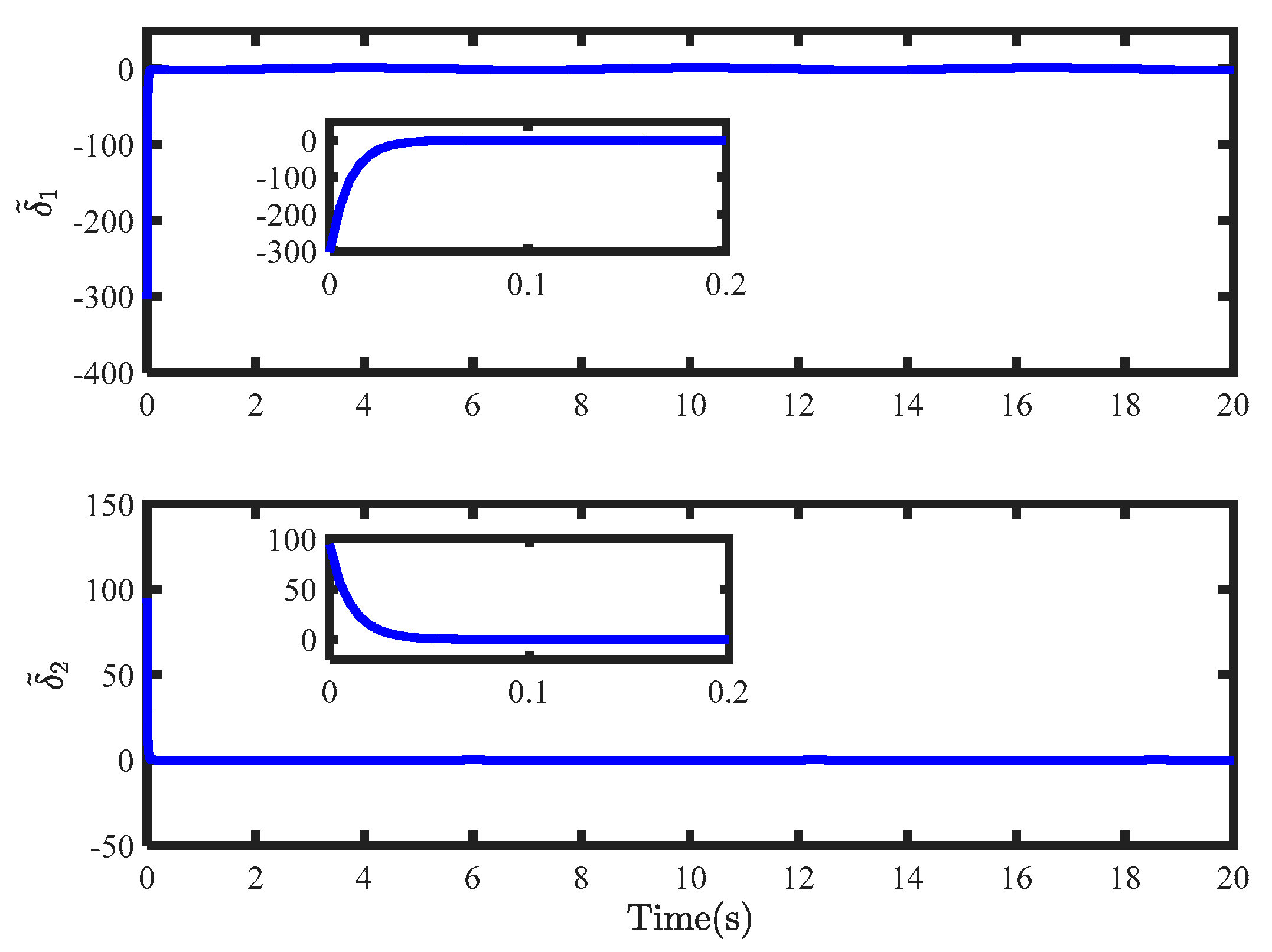
The simulation results for a period of 20 s are shown from Figure 2, Figure 3, Figure 4, Figure 5, Figure 6, Figure 7 and Figure 8. Figure 2 gives the simulation results of the system state and the reference command, which indicates that the state can accurately track the reference command within 4 s. The tracking errors enter the steady state quickly, which can be due to the estimation from the USDE, as shown in Figure 3. Lumped disturbances can be approximated precisely within 0.1 s.

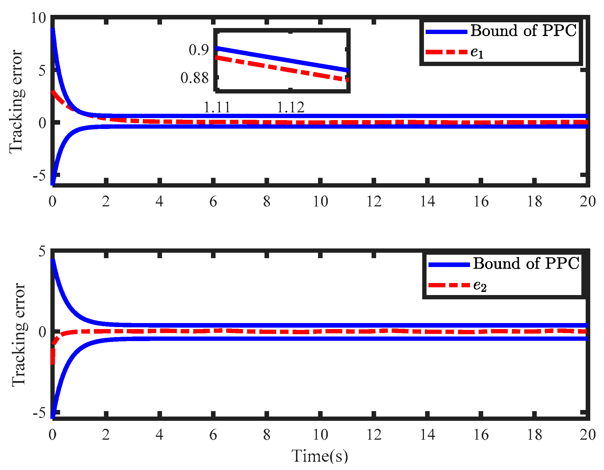
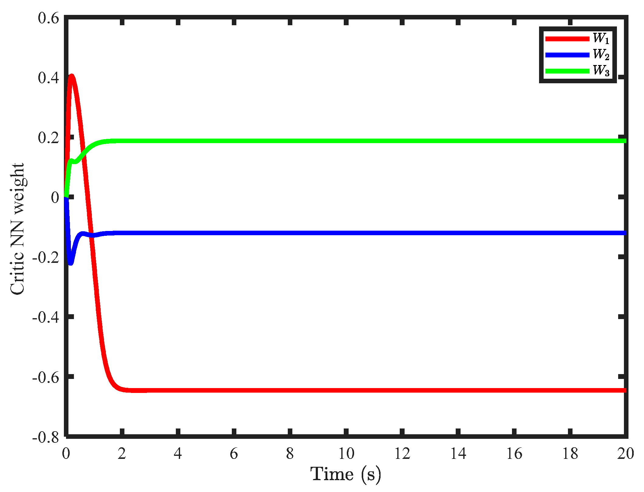
The control inputs of the proposed controller are described in Figure 4, which include the feedback control and the optimal control. Figure 5 describes the simulation results of the tracking error and asymmetric output performance constraints. It can be found that the tracking errors converged to a specified asymmetric envelope, which indicated that the designed controller with an optimal preset performance can make tracking errors converge to zero within a predetermined convergence rate. The stability of the closed-loop system hinged on the weight of the critic NN, as illustrated in Figure 6, which showed the approximation of weight can converge to the ideal weight within 2 s.

In order to illustrate the superiority of the proposed controller in achieving preset performance, it was compared with the optimal controller based on the traditional value function in [32], which is named WPPC. Noting that the controller in [32] is based on a fixed-time disturbance observer, we set the feedback controller based on a USDE for the sake of fair comparison. Figure 7 shows the simulation results of the tracking error and the PPC envelope. Although the system state tracked the reference command successfully, the tracking errors could not evolve within the envelope, and the transient performance could not be guaranteed to meet the output constraints. This indicates that the convergence rate of the tracking error was slower than that of the specified convergence rate and the predetermined performance could not be guaranteed. Figure 8 compares the value functions of the two controllers for 20 s. In contrast, the value function of the new controller decreased by 6% compared to the optimal controller without taking into preset performance account. Therefore, the new controller can ensure that the tracking error meets the output performance constraints while its value function is smaller.

Example 2.

Noting that the trajectory tracking problem of the quadrotor can be affected by uncertain dynamic drift and disturbance induced by wind, the effectiveness of the proposed control is carried on a quadrotor [3,31]. Noting that position and attitude loops are considered in [3,31], the position dynamic of the quadrotor is considered as:

$$\{\begin{array}{l}\dot{\mathit{p}}=\mathit{v}\\ \dot{\mathit{v}}=\left(-g{\mathit{h}}_3-\mathbf{\prod }\mathit{v}\right)/m+\mathit{u}+{\mathit{d}}_v\end{array}$$

(56)

where parameters of the model are listed in

Table 1. Parameters of the quadrotor attitude dynamics.

Section	Values
Mass	2
Inertia moment matrix	$\mathrm{diag}\left(\right[0.01,0.01,0.01\left]\right)$
Disturbances	${[\sin (4t)+\cos (2t)-\sin (t);\cos (4t)+\sin (2t)-\cos (t);\sin (3t)\cos (2t)-\cos (t)]}^T$

. The given reference trajectory is ${\mathit{p}}^d={[10(1-\cos (0.1\pi t)),5\sin (0.2\pi t),9(1-e^{-0.3t})]}^T$.

To carry out the proposed controller on Equation (53), we reformulate it as:

$$\dot{\mathit{x}}=\mathit{f}(\mathit{x})+\mathit{g}(\mathit{x})\mathit{u}+\mathit{d}(t)$$

(57)

where

$$\mathit{x}=\left[\begin{array}{l}\mathit{p}\\ \mathit{v}\end{array}\right],\mathit{f}(\mathit{x})=\left[\begin{array}{c}\mathit{v}\\ \left(-g{\mathit{h}}_3-\mathbf{\prod }\mathit{v}\right)/m\end{array}\right],\mathit{g}(\mathit{x})=\left[\begin{array}{l}\mathbf{0}\\ \mathit{I}\end{array}\right]$$

(58)

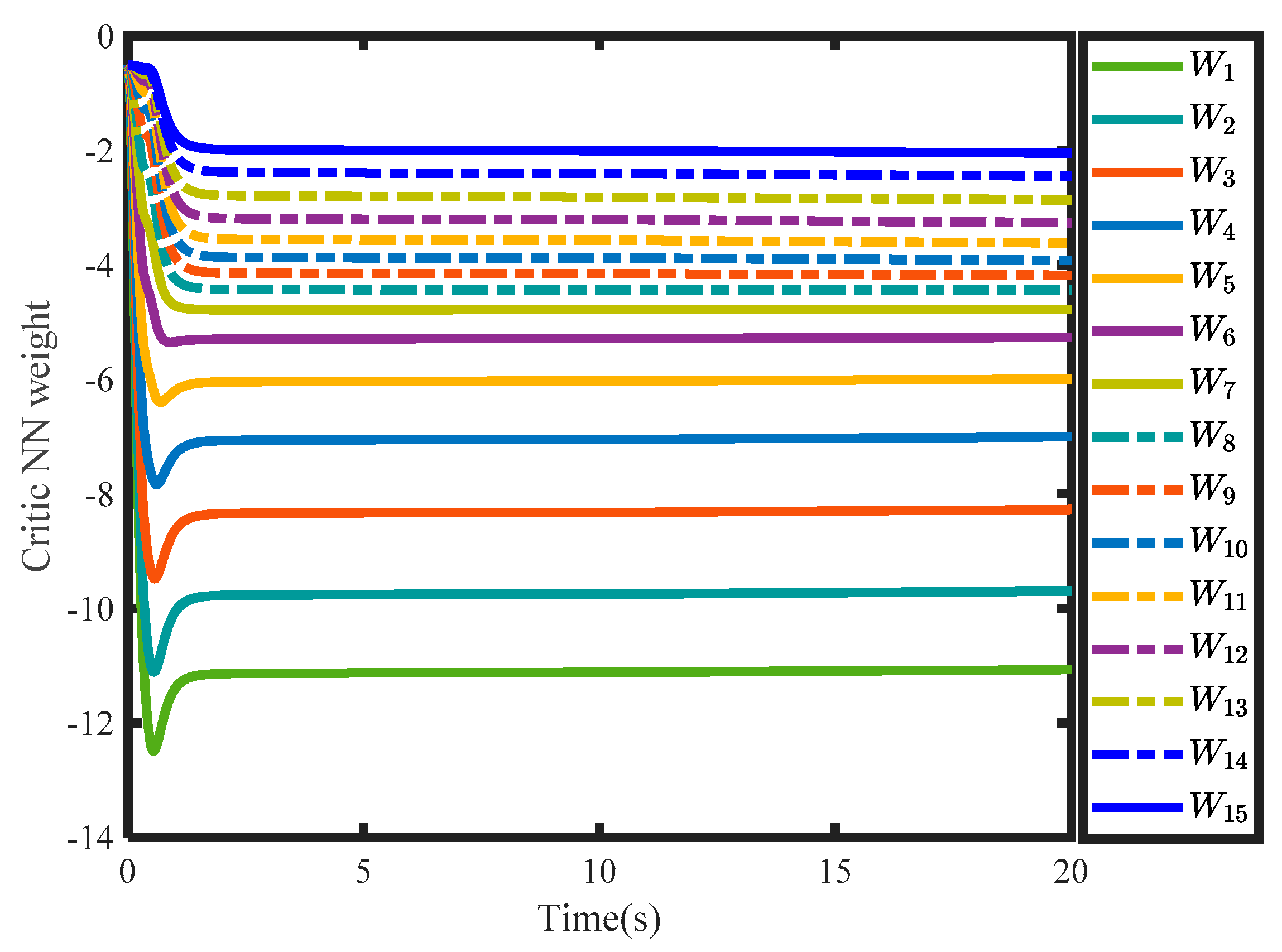
For approximating the optimal control, the critic NN is structured with 15 neurons with [−5,5]. For the initial position and weight, we choose the following parameters: $\mathit{p}(0)={[-5,3,2]}^T$ and ${\mathit{W}}_0=\mathbf{0}$. The other controller parameters are listed in

Table 2. Parameters of the controllers.

Section	Values
USDE	$k=0.01$
PPC	${\underset{\_}{l}}^{px}=2.5,{\overline{l}}^{px}=1.5,{\vartheta }_{{}_0}^{px}=5,{\vartheta }_{{}_{\infty }}^{px}=0.2,a^{px}=2$ ${\underset{\_}{l}}^{py}=2.5,{\overline{l}}^{py}=3,{\vartheta }_{{}_0}^{px}=5,{\vartheta }_{{}_{\infty }}^{px}=0.2,a^{px}=3$ ${\underset{\_}{l}}^{pz}=2.5,{\overline{l}}^{pz}=2,{\vartheta }_{{}_0}^{pz}=5,{\vartheta }_{{}_{\infty }}^{pz}=0.2,a^{pz}=3$ ${\underset{\_}{l}}^{vx}=2,{\overline{l}}^{vx}=1.5,{\vartheta }_{{}_0}^{vx}=8,{\vartheta }_{{}_{\infty }}^{vx}=0.2,a^{vx}=3$ ${\underset{\_}{l}}^{vy}=1.3,{\overline{l}}^{vy}=1.5,{\vartheta }_{{}_0}^{vy}=10,{\vartheta }_{{}_{\infty }}^{vy}=0.2,a^{vy}=3$ ${\underset{\_}{l}}^{vz}=0.6,{\overline{l}}^{vz}=0.8,{\vartheta }_{{}_0}^{vz}=8,{\vartheta }_{{}_{\infty }}^{vz}=0.2,a^{vz}=3$
Control gain	$\mathit{K}=\mathrm{d}\mathrm{i}\mathrm{a}\mathrm{g}[2,2,2,2,2,2]$

.

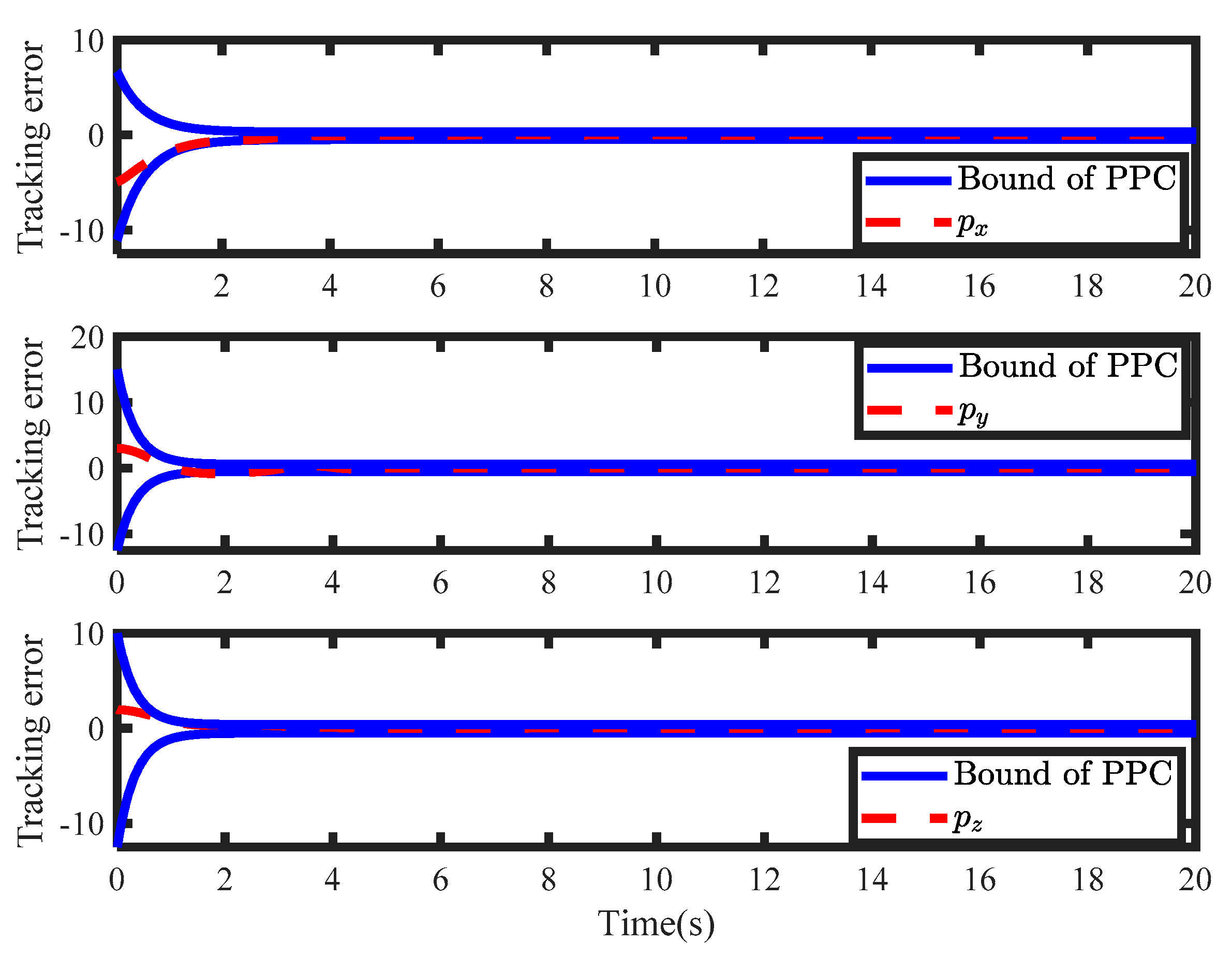
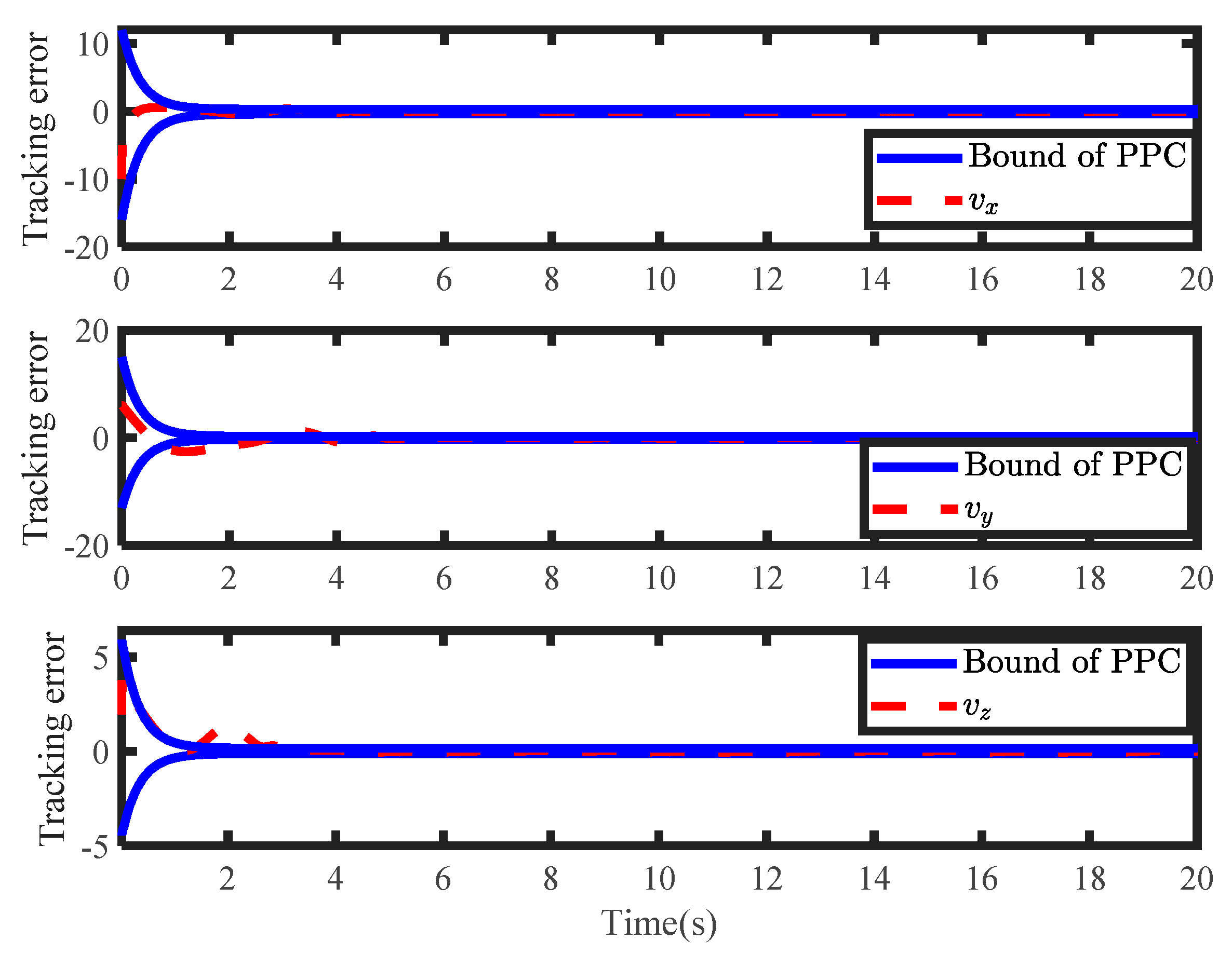
The performance of the proposed controller was discussed as follows. Figure 9 and Figure 10 show the tracking performances of the position and the velocity. It can be found that tracking errors evolved the predefined constraints. By running the novel value function, tracking errors converged to zero within the convergence rate. During the controller design, the weight of the critic NN is crucial for solving the HJB equation. Figure 11 gives the convergence of weight, which is essential for the stability of the closed-loop system. To verify the advantage of the novel value function, the optimal tracking controller in [32] was executed for System (54). In the position loop, the tracking errors of the position and the velocity are shown in Figure 12 and Figure 13, which indicates the tracking errors could not evolve the predefined envelope by minimizing the value function without the PPC constraints. Therefore, the effectiveness of the proposed optimal control was verified to deal with prescribed performance. Noting that the proposed controller and the optimal tracking controller in [32] are based on simulation, we will further consider experimental validation based on physical systems to verify the feasibility of the proposed method, where complete response associated is impossible.

6. Conclusions

In this paper, an optimal tracking control with output constraints was proposed to ensure tracking errors with prescribed performance. The perturbation estimation error was introduced into critic-only ADP, and the novel value function was run within a critic-only ADP framework to derive the optimal control. It proved that the tracking error can be realized in the specified envelope of the PPC. The numerical simulation verified that the designed controller can achieve tracking errors with prescribed performance on the quadrotor trajectory tracking problem and a class of second-order nonlinear systems. However, actuator saturation may limit the control input, which makes it difficult to guarantee prescribed performance. We will focus on the optimal tracking controller for uncertain nonlinear systems with prescribed performance under actuator saturation.

References

1. Vu, Q.V.; Dinh, T.A.; Nguyen, T.V.; Tran, H.V.; Le, H.X.; Pham, H.V.; Kim, T.D.; Nguyen, L. An adaptive hierarchical sliding mode controller for autonomous underwater vehicles. Electronics 2021, 10, 2316. [Google Scholar] [CrossRef]
2. Liang, L.; Liu, H.; Li, X.; Zhu, X.; Lan, B.; Liu, Y.; Wang, X. Model-based coordinated trajectory tracking control of skid-steer mobile robot with timing-belt servo system. Electronics 2023, 12, 699. [Google Scholar] [CrossRef]
3. Shao, X.; Yue, X.; Li, J. Event-triggered robust control for quadrotors with preassigned time performance constraints. Appl. Math. Comput. 2021, 392, 125667. [Google Scholar] [CrossRef]
4. Li, S.; Ahn, C.K.; Guo, J.; Xiang, Z. Neural-network approximation-based adaptive periodic event-triggered output-feedback control of switched nonlinear systems. IEEE Trans. Cybern. 2020, 51, 4011–4020. [Google Scholar] [CrossRef] [PubMed]
5. Li, Y.; Li, K.; Tong, S. Adaptive neural network finite-time control for multi-input and multi-output nonlinear systems with positive powers of odd rational numbers. IEEE Trans. Neural Netw. Learn. Syst. 2019, 31, 2532–2543. [Google Scholar] [CrossRef]
6. Tatlicioglu, E.; Yilmaz, B.M.; Savran, A.; Alci, M. Adaptive fuzzy logic with self-adjusting membership functions based tracking control of surface vessels. Ocean. Eng. 2022, 253, 111129. [Google Scholar] [CrossRef]
7. Tang, J.; Dang, Z.; Deng, Z.; Li, C. Adaptive fuzzy nonlinear integral sliding mode control for unmanned underwater vehicles based on ESO. Ocean. Eng. 2022, 266, 113154. [Google Scholar] [CrossRef]
8. Li, Y.; Li, K.; Tong, S. An observer-based fuzzy adaptive consensus control method for nonlinear multiagent systems. IEEE Trans. Fuzzy Syst. 2022, 30, 4667–4678. [Google Scholar] [CrossRef]
9. Chen, M.; Xiong, S.; Wu, Q. Tracking flight control of quadrotor based on disturbance observer. IEEE Trans. Syst. Man Cybern. 2019, 51, 1414–1423. [Google Scholar] [CrossRef]
10. Guo, K.; Shi, P.; Wang, P.; He, C.; Zhang, H. Non-singular terminal sliding mode controller with nonlinear disturbance observer for robotic manipulator. Electronics 2023, 12, 849. [Google Scholar] [CrossRef]
11. Kukurowski, N.; Pazera, M.; Witczak, M. Fault-tolerant tracking control for a descriptor system under an unknown input disturbances. Electronics 2021, 10, 2247. [Google Scholar] [CrossRef]
12. Huang, Y.; Wu, J.; Na, J.; Han, S.; Gao, G. Unknown system dynamics estimator for active vehicle suspension control systems with time-varying delay. IEEE Trans. Cybern. 2021, 52, 8504–8514. [Google Scholar] [CrossRef] [PubMed]
13. Na, J.; Jing, B.; Huang, Y.; Gao, G.; Zhang, C. Unknown system dynamics estimator for motion control of nonlinear robotic systems. IEEE Trans. Ind. Electron. 2019, 67, 3850–3859. [Google Scholar] [CrossRef]
14. Wang, S.; Tao, L.; Chen, Q.; Na, J.; Ren, X. USDE-based sliding mode control for servo mechanisms with unknown system dynamics. IEEE/ASME Trans. Mech. 2020, 25, 1056–1066. [Google Scholar] [CrossRef]
15. Khodamipour, G.; Khorashadizadeh, S.; Farshad, M. Adaptive formation control of leader-follower mobile robots using reinforcement learning and the fourier series expansion. ISA Trans. 2023, in press. [Google Scholar] [CrossRef]
16. Bao, C.; Wang, P.; He, R.; Tang, G. Observer-based optimal control method combination with event-triggered strategy for hypersonic morphing vehicle. Aerosp. Sci. Technol. 2023, 136, 108219. [Google Scholar] [CrossRef]
17. Hua, H.; Fang, Y. A novel reinforcement learning-based robust control strategy for a quadrotor. IEEE Trans. Ind. Electron. 2022, 70, 2812–2821. [Google Scholar] [CrossRef]
18. Bechlioulis, C.P.; Rovithakis, G.A. Robust adaptive control of feedback linearizable MIMO nonlinear systems with prescribed performance. IEEE Trans. Autom. Control 2008, 53, 2090–2099. [Google Scholar] [CrossRef]
19. Wang, N.; Gao, Y.; Zhang, X. Data-driven performance-prescribed reinforcement learning control of an unmanned surface vehicle. IEEE Trans. Neural Netw. Learn. Syst. 2021, 32, 5456–5467. [Google Scholar] [CrossRef]
20. Liu, H.; Cheng, Q.; Xiao, J.; Hao, L. Data-driven optimal tracking control for SMA actuated systems with prescribed performance via reinforcement learning. Mech. Syst. Signal Process. 2022, 177, 109191. [Google Scholar] [CrossRef]
21. Chen, H.; Yan, H.; Wang, Y.; Xie, S.; Zhang, D. Reinforcement learning-based close formation control for underactuated surface vehicle with prescribed performance and time-varying state constraints. Ocean. Eng. 2022, 256, 111361. [Google Scholar] [CrossRef]
22. Wang, X.; Wang, Q.; Sun, C. Prescribed performance fault-tolerant control for uncertain nonlinear MIMO system using actor–critic learning structure. IEEE Trans. Neural Netw. Learn. Syst. 2021, 33, 4479–4490. [Google Scholar] [CrossRef] [PubMed]
23. Zhang, S.; Huang, C.; Ji, K.; Zhang, H. Prescribed performance incremental adaptive optimal fault-tolerant control for nonlinear systems with actuator faults. ISA Trans. 2022, 120, 99–109. [Google Scholar] [CrossRef] [PubMed]
24. Li, D.; Dong, J. Performance-constrained fault-tolerant DSC based on reinforcement learning for nonlinear systems with uncertain parameters. Appl. Math. Comput. 2023, 443, 127759. [Google Scholar] [CrossRef]
25. Liu, G.; Sun, N.; Yang, T.; Fang, Y. Reinforcement learning-based prescribed performance motion control of pneumatic muscle actuated robotic arms with measurement noises. IEEE Trans. Syst. Man Cybern. 2022, in press. [Google Scholar] [CrossRef]
26. Yan, L.; Liu, Z.; Chen, C.L.P.; Zhang, Y.; Wu, Z. Optimized adaptive consensus control for multi-agent systems with prescribed performance. Inf. Sci. 2022, 613, 649–666. [Google Scholar] [CrossRef]
27. Ouyang, Y.; Sun, C.; Dong, L. Actor-critic learning based coordinated control for a dual-arm robot with prescribed performance and unknown backlash-like hysteresis. ISA Trans. 2022, 126, 1–13. [Google Scholar] [CrossRef]
28. Luo, A.; Xiao, W.; Li, X.M.; Yao, D.; Zhou, Q. Performance-guaranteed containment control for pure-feedback multi agent systems via reinforcement learning algorithm. Int. J. Robust Nonlinear Control. 2022, 32, 10180–10200. [Google Scholar] [CrossRef]
29. Peng, Z.; Ji, H.; Zou, C.; Kuang, Y.; Cheng, H.; Shi, K.; Ghosh, B. Optimal H tracking control of nonlinear systems with zero-equilibrium-free via novel adaptive critic designs. Neural Netw. 2023, 164, 105–114. [Google Scholar] [CrossRef]
30. Huo, Y.; Wang, D.; Qiao, J.; Li, M. Adaptive critic design for nonlinear multi-player zero-sum games with unknown dynamics and control constraints. Nonlinear Dyn. 2023, 111, 11671–11683. [Google Scholar] [CrossRef]
31. Vamvoudakis, K.; Lewis, F. Online actor–critic algorithm to solve the continuous-time infinite horizon optimal control problem. Automatica 2010, 46, 878–888. [Google Scholar] [CrossRef]
32. Liu, H.; Li, B.; Xiao, B.; Ran, D.; Zhang, C. Reinforcement-learning-based tracking control for a quadrotor unmanned aerial vehicle under external disturbances. Int. J. Robust Nonlinear Control. 2022, in press. [Google Scholar] [CrossRef]
Figure 1. The diagram of the whole controller.
Electronics 12 02545 g001
Figure 2. The tracking performance.
Electronics 12 02545 g002
Figure 3. The estimation errors of lumped disturbances.
Electronics 12 02545 g003
Figure 4. The control inputs.
Electronics 12 02545 g004
Figure 5. The tracking errors with the PPC.
Electronics 12 02545 g005
Figure 6. The weight of the critic NN (Example 1).
Electronics 12 02545 g006
Figure 7. The tracking errors with the WPPC.
Electronics 12 02545 g007
Figure 8. Comparison of cost functions.
Electronics 12 02545 g008
Figure 9. The tracking errors of the position.
Electronics 12 02545 g009
Figure 10. The tracking errors of the velocity.
Electronics 12 02545 g010
Figure 11. The weight of the critic NN (Example 2).
Electronics 12 02545 g011
Figure 12. The tracking errors of the position [32].
Electronics 12 02545 g012
Figure 13. The tracking errors of the velocity [32].
Electronics 12 02545 g013