AV PV-RCNN: Improving 3D Object Detection with Adaptive Deformation and VectorPool Aggregation

Abstract

Three-dimensional object detection has attracted more and more attention from industry and academia due to its wide application in various fields such as autonomous driving and robotics. Currently, the refinement methods used by advanced two-stage detectors cannot fully adapt to different object scales, different point cloud densities, partial deformation and clutter, and excessive resource consumption. We propose a point cloud-based 3D object detection method that can adapt to different object scales and aggregate local features with less resources. The method first passes through an adaptive deformation module based on a 2D deformable convolutional network, which can adaptively collect instance-specific features from where the information content exists. Secondly, through a VectorPool aggregation module, this module can better aggregate local point features with less resource consumption. Finally, through a context fusion module, the key points can filter out relevant context information for the refinement stage. Our proposed detection method not only achieves better accuracy on the KITTI dataset, but also consumes less resources than the original detectors and has faster inference speed.

1. Introduction

With the continuous development of application fields such as autonomous driving, robotics and augmented reality, the demand for accurate, fast and reliable 3D object detection technology is becoming more and more urgent. Three-dimensional object detection aims to identify and locate different types of objects from a three-dimensional scene. Compared with traditional 2D object detection, 3D object detection can provide more accurate object position information and is also more robust because it is not easily disturbed by factors such as light and shadow. However, 3D object detection faces many technical challenges. Due to the sparsity and irregularity of point cloud data, it is very challenging to directly apply 2D object detection technology to process point clouds.

In order to deal with these challenges, most of the existing 3D detection methods can be divided into three categories according to the representation of point clouds: grid-based methods, point-based methods, and combination of grid-based and point-based methods. Grid-based methods [1,2,3,4,5,6,7] usually convert irregular point clouds into regular representations, such as 3D voxels or 2D bird’s eye views, which can be efficiently processed by 3D or 2D convolutional neural networks (CNNs) to learn point features for 3D detection. Point-based methods [8,9,10,11,12,13,14] usually directly extract discriminative features from raw point clouds for 3D detection. Grid-based methods are generally more computationally efficient, but they suffer from information loss, which may reduce localization accuracy for the location of fine details. Different from this, point-based methods are usually more computationally expensive, but with point set abstraction, a larger receptive field is easily obtained, which provides more comprehensive information for 3D object detection. The combination of grid-based and point-based methods [15,16,17] combines the advantages of high computational efficiency of the grid-based method with the flexible advantages of the point-based method, which not only improves the computational efficiency of the network, but also fully obtains rich context information.

The above three categories of 3D object detection algorithms process point clouds from different aspects, especially the combination of grid-based and point-based methods, the most typical of which is the PV-RCNN [15] network, in the voxel feature extraction in the down-sampling stage, PV-RCNN mainly uses the set abstraction operation of PointNet++ [9] to extract voxel features at multiple scales, although it has achieved certain results, it can not fully adapt to different size objects, different point cloud density, clutter and other problems. For example, when extracting voxel features, sometimes the position of the sampled keypoints is far away from the object or the center of the object, and the features of the object cannot be extracted well, if the keypoints can be shifted closer to the object or the center of the object by learning the features of the surrounding neighborhood, then the surrounding neighborhood features acquired by the keypoints will be more suitable for objects of different sizes. When extracting keypoint features in the second stage of PV-RCNN, the set abstraction operation of PointNet++ is used to extract keypoint features at multiple scales, but it makes processing large-scale point clouds very resource-intensive and time-consuming, and the maximum pooling operation in set abstraction discards local spatial distribution information, resulting in the lack of local spatial information in the features obtained by grid points.

In order to solve the problem that PV-RCNN cannot fully adapt to different object scales, different point cloud densities, clutter, and excessive resource consumption, we were first inspired by deformable convolution [18] and Deformable PV-RCNN [16], and found that sampling points can be shifted to places with more information according to the surrounding neighborhood information, so as to extract the features of specific instances and adapt to objects of different sizes; secondly, inspired by the encoding of local spatial information in PV-RCN [17], PV-RCNN++ uses independent kernel weights and channels to aggregate features of local points, consuming less resources; and finally, inspired by the gating mechanism, the gating mechanism can filter out more prominent features and filter out insignificant features, thereby suppressing clutter. To this end, we propose a point cloud-based 3D object detection method that can fully adapt to different object scales and aggregate local features with less resources. The main contributions of this paper are as follows:

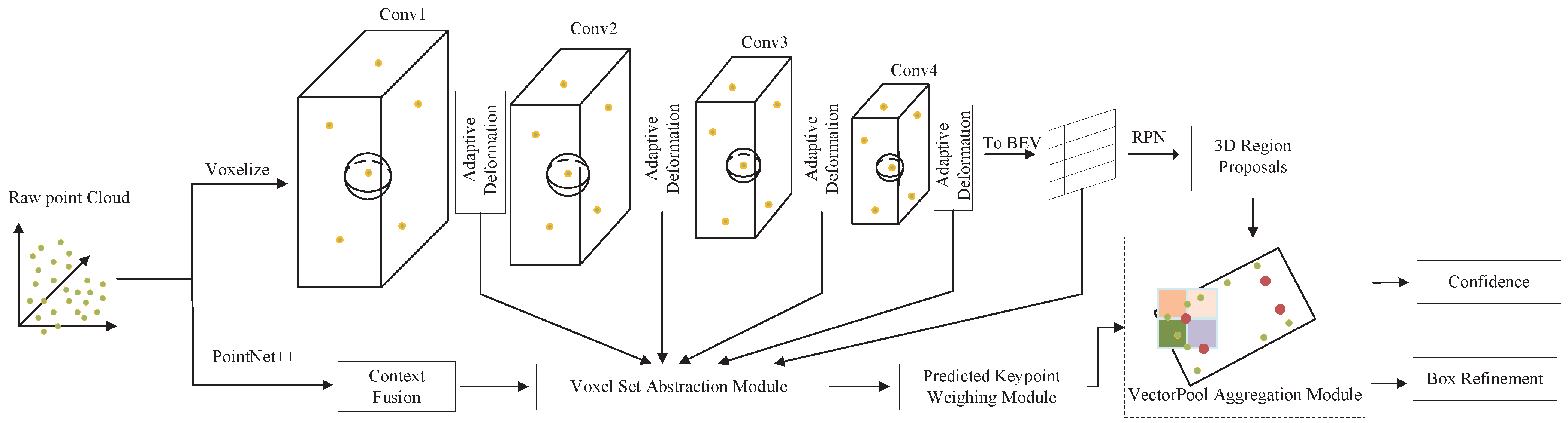
• Replacing the set abstraction of the Voxel Set Abstraction Module in PV-RCNN with the adaptive deformation module. Through the adaptive deformation module, the keypoints can be aligned with the most distinctive areas, and the most prominent features of objects of different scales can be adaptively gathered and focused, so that the model can detect uneven point cloud density better.
• Replacing the set abstraction in the RoI-grid pooling module in PV-RCNN with the VectorPool aggregation module. The VectorPool aggregation module uses independent kernel weights and channels to encode position-sensitive local features in different regions centered on grid points, which not only preserves the spatial structure of grid points well, but also saves the consumption of computing resources.
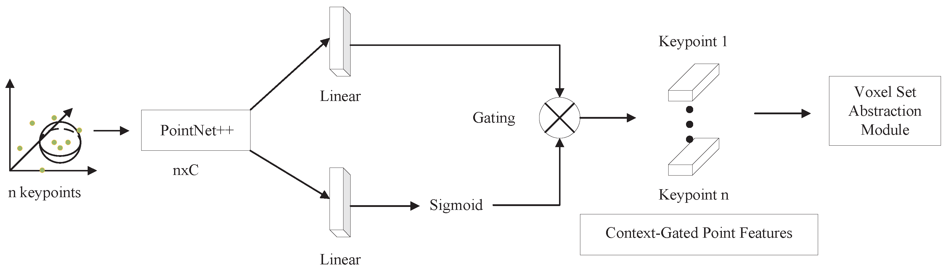
• Using the context fusion module to perform feature selection on keypoints obtained directly from PointNet++ in PV-RCNN. Representative and discriminative features can be dynamically selected from local evidence through the context gating mechanism, which adaptively highlights relevant contextual features, thus facilitating the optimization of more accurate 3D candidate boxes.

2. Related Work

3D Object Detection with Grid-based Methods. In order to deal with irregular point clouds, most methods usually map the point cloud to a grid of bird’s eye view or voxelization. MV3D [1] projects point clouds into a 2D bird’s eye view grid and places a large number of predefined 3D anchor points for generating 3D bounding boxes; AVOD [2] extends MV3D by introducing image features in the proposal generation stage, improve 3D detection accuracy; VoxelNet [3] first voxelizes the entire point cloud, then uses PointNet [8] to extract the features of each voxel, and finally generates a detection frame through RPN; compared to VoxelNet, SECOND [4] applies sparse convolution to replace 3D convolution operation, so as to achieve the effect of reducing the amount of calculation and improving the training speed; PointPillars [5] divides the point cloud into columns, reduces the number of voxels that need to be processed, and improves the detection speed; VoTr [6] is a transformer-based 3D backbone network that uses a deformed attention mechanism that can effectively operate on empty and non-empty voxel positions, preserves the spatial position encoding, and can be used as an alternative to standard sparse convolutional layers; CenterPoint [7] uses the idea of Anchor-free to predict the center point of the 3D frame in the first stage and regress its size, direction and speed, while the second stage uses the center point feature to return the score of the detection frame and optimize it.

3D Object Detection with Point-based Methods. In addition to grid processing of point clouds, PointNet [8] and PointNet++ [9] directly process the point cloud for point cloud classification and segmentation, and can also be used as the backbone network for feature extraction; F-PointNet [10] first proposed the method of using cones to achieve 3D target detection; firstly, the candidate area is generated by an excellent 2D target detection algorithm, and the 3D view cone is extracted by combining the depth information of the candidate area, then the 3D instance is segmented by PointNet [8], and finally the coordinates are transformed by the T-Net network, so that the central axis of the viewing frustum orthogonal to the image plane and predict the final 3D bounding box; the first stage of PointRCNN [11] uses PointNet++ [9] to extract point cloud features, divides the point cloud of the entire scene into foreground points and background points, and generates a small number of 3D candidate boxes from the foreground points, while the second stage converts the pooled points of each candidate box into canonical coordinates, so as to better learn local spatial features to optimize 3D boxes; STD [12] uses point-based spherical anchors boxes to generate more accurate candidate frames, which reduces the number of generated anchor boxes and greatly reduces the amount of calculation; VoteNet [13] proposed a Hough voting strategy to better group object features; 3D-SSD [14] adopts a farthest point sampling method based on feature distance, and excludes a large number of background points by combining semantic information, in order to avoid certain redundancy caused by completely using feature distance-based sampling; therefore, they choose to combine the Euclidean distance and the method of sampling the farthest point based on feature distance, and remove the very time-consuming FP module and optimization module in PointNet++, which greatly reduces the calculation loss.

3D Object Detection with combination of grid-based and point-based methods. PV-RCNN [15] combines voxel-based feature learning and point-network-based feature learning to generate high-quality 3D pre-selection boxes and capture more accurate contextual information through flexible receptive fields, thereby improving 3D detection performance. Deformable PV-RCNN [16] improves the detection performance of long-distance targets by collecting unevenly distributed context information. PV-RCNN++ [17] uses sector-proposal-centered sampling and local point feature aggregation to improve the model. The performance and inference speed not only speed up the running speed of the model, but also improve the detection performance of the model.

3. Method

In this section, we focus on introducing the network structure of our model, which is improved based on PV-RCNN, as shown in Figure 1.

We designed a network that can fully adapt to different object sizes and reduce computing resource consumption. First, the set abstraction for voxel feature extraction in PV-RCNN is replaced with an adaptive deformation module, which can aggregate the instance features of object features of different scales on the keypoints; secondly, the set abstraction in the aggregation operation of the keypoints features in the second stage of PV-RCNN is replaced by the VectorPool aggregation module to display and encode the spatial structure information of the keypoints features; finally, the context fusion module is used to filter the keypoints features obtained directly from PointNet++ in PV-RCNN, dynamically select representative and discriminative features from local evidence, and adaptively highlight relevant contextual features. In this section, a brief introduction to the original PV-RCNN model is given first, followed by a detailed description of the voxel set abstraction module, deformable convolution, adaptive deformation module, context fusion module, roI-grid pooling module, and VectorPool aggregation module.

3.1. PV-RCNN

PV-RCNN is the benchmark model of our work. As shown in Figure 2, it is a two-stage 3D object detection model based on the combination of grid and points. PV-RCNN uses 3D sparse convolution as the backbone for feature extraction and 3D candidate boxes generation, in order to make full use of the characteristics of the entire scene, PV-RCNN proposes two methods, namely voxel-to-keypoint feature encoding and keypoint-to-grid point feature extraction. Voxel-to-keypoint feature encoding is mainly realized through the Voxel Set Abstraction Module, 3D sparse convolution performs 1, 2, 4, and 8 times downsampling processing on the point cloud, and each downsampled voxel feature represents the whole scene, the keypoints are obtained by directly performing the farthest point sampling algorithm (FPS) on the point cloud, the keypoints use the set abstraction in PointNet++ to extract the voxel features in the whole scene, so that the voxels obtained by each downsampling feature are encoded into a set of keypoints. The keypoint-to-grid point feature extraction is mainly realized through the RoI-grid pooling module. According to the generated 3D candidate boxes, 6 × 6 × 6 grid points are selected, and the grid points use the set abstraction in PointNet++ to extract the keypoints features around the grid points, so that the grid points have rich features of the entire scene. Finally, PV-RCNN predicts the final 3D boxes and confidence according to the features of the grid points.

3.2. Voxel Set Abstraction Module

The voxel set abstraction (VSA) module is used to encode the voxel features in the scene in the 3D sparse convolution into a set of keypoints, that is, each keypoint uses the set abstraction operation proposed by PointNet++ [9] to aggregate voxel features at multiple scales. Specifically, the FurthestPoint-Sampling (FPS) algorithm is used to sample n keypoints $K=\{p_1,\cdots ,p_n\}$ from the entire point cloud P, where in the KITTI dataset $n=2048$, the keypoints can be evenly distributed in the entire point by the FurthestPoint-Sampling (FPS) algorithm, it can represent the entire point cloud scene, the keypoints are surrounded by voxel features obtained through 3D sparse convolution, and the keypoints directly use the set abstraction in PointNet++ to perform multi-scale feature extraction on the surrounding voxel features.

Specifically, ${\mathcal{F}}^{\left(l_k\right)}=\{f_1^{\left(l_k\right)},\cdots ,f_{N_k}^{\left(l_k\right)}\}$ is represented as the non-empty voxel feature vector set of the k-th layer of the 3D sparse convolution, and ${\mathcal{V}}^{l_k}=\{v_1^{\left(l_k\right)},\cdots ,v_{N_k}^{\left(l_k\right)}\}$ is represented as the three-dimensional coordinates of the non-empty voxel of the k-th layer of the 3D sparse convolution, where $N_k$ is the number of non-empty voxels in the k-th layer of 3D sparse convolution, for each keypoint $p_i$, we first search for non-empty voxels within the radius $r_k$ of the k-th layer to obtain the voxel-level feature vector set of the keypoint $p_i$ as:

$$\begin{array}{c}\hfill S_i^{\left(l_k\right)}=\left\{{\left[f_j^{\left(l_k\right)};v_j^{\left(l_k\right)}-p_i\right]}^T\left|\begin{array}{c}\parallel v_j^{\left(l_k\right)}-p_i{\parallel }^2<r_k,\\ \forall v_j^{\left(l_k\right)}\in {\mathcal{V}}^{\left(l_k\right)},\\ \forall f_j^{\left(l_k\right)}\in {\mathcal{F}}^{\left(l_k\right)}\end{array}\right\}\right.\end{array}$$

(1)

It concatenates the local relative coordinates $v_j^{\left(l_k\right)}-p_i$ to represent the relative position of the semantic voxel feature $f_j^{\left(l_k\right)}$. The voxel features in the adjacent voxel set $S_i^{\left(l_k\right)}$ of $p_i$ are then transformed by Set Abstraction in PointNet++ [9] to generate the features of the keypoint $p_i$:

$$\begin{array}{c}\hfill f_i^{\left(p{v}_k\right)}=max\left\{G\left(\mathcal{M}\left(S_i^{\left(l_k\right)}\right)\right)\right\}\end{array}$$

(2)

where $\mathcal{M}(·)$ represents random sampling of at most $T_k$ voxels from the adjacent voxel set $S_i^{l_k}$ to save computation, and $G(·)$ represents a simple MLP network. $max\{·\}$ represents the maximum pooling operation on all adjacent voxel features $S_i^{l_k}$ along all channels of the voxel.

Finally, by concatenating the keypoint features of all layers, the final feature of the keypoint $p_i$ is obtained:

$$\begin{array}{c}\hfill f_i^{\left(pv\right)}=\left[f_i^{\left(p{v}_1\right)},f_i^{\left(p{v}_2\right)},f_i^{\left(p{v}_3\right)},f_i^{\left(p{v}_4\right)}\right],fori=1,\cdots ,n\end{array}$$

(3)

The above is the whole content of the voxel set abstraction module. When using the set abstraction of PointNet++ [9] to extract the surrounding neighborhood features, multiple scales are used to extract the surrounding voxel features. Although good results have been achieved, it cannot fully adapt to problems such as different object scales, different point cloud densities, clutter, etc., resulting in some objects not being detected. For example, sometimes the keypoints are far from the object or the center of the object, and the features extracted by the key points cannot well-represent the shape of the object and cannot fully adapt to objects of different sizes, which may easily cause wrong detection results and lead to a decrease in accuracy.

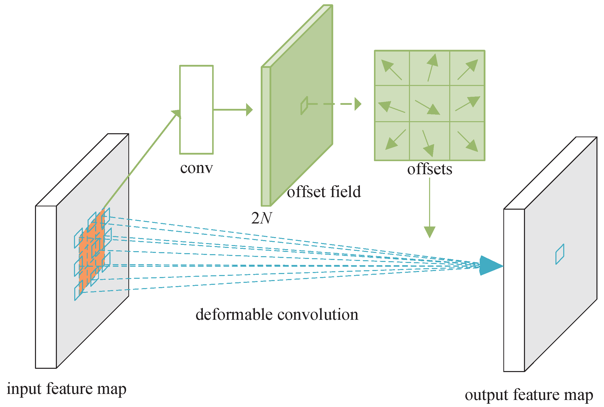
3.3. Deformable Convolution

In 2D object detection, deformable convolution has shown its powerful ability. Deformable convolution can adaptively shift the position of sampling points to a place with richer feature information, so as to sample richer feature information and fully adapt to objects of different sizes, as shown in Figure 3.

The core of 2D convolution is the convolution kernel R, which is used to sample the feature map x. The convolution kernel determines the size of the receptive field, such as the 3 × 3 kernel:

$$\begin{array}{c}\hfill R=\left\{\right(-1,1),(-1,0),\cdots ,(0,1),(1,1\left)\right\}\end{array}$$

(4)

In order to achieve each position $p_0$ on the output feature map y, we have

$$\begin{array}{c}\hfill y\left(p_0\right)=\sum _{p_n\in R}w\left(p_n\right)·x(p_0+p_n)\end{array}$$

(5)

where $p_n$ is each position in the convolution kernel R.

In deformable convolution, the convolution kernel R uses the offset $\{\Delta p_n|n=1,\cdots ,N\}$ to obtain a new sampling position, where $N=\left|R\right|$. Equation (5) becomes:

$$\begin{array}{c}\hfill y\left(p_0\right)=\sum _{p_n\in R}w\left(p_n\right)·x(p_0+p_n+\Delta p_n)\end{array}$$

(6)

Now, the position of the convolution kernel sampling is $p_n+\Delta p_n$. Since the offset $\Delta p_n$ is usually a fraction, Equation (6) is realized by bilinear interpolation as:

$$\begin{array}{c}\hfill x\left(p\right)=\sum _{q}E(q,p)·x\left(q\right)\end{array}$$

(7)

where p represents any (fractional) position ($p=p_0+p_n+\Delta p_n$ in Equation (6)), q enumerates all integral spatial positions in the feature map x, and $E(·,·)$ is the bilinear interpolation kernel. Note that E is two-dimensional. It is split into two 1D kernels:

$$\begin{array}{c}\hfill E(q,p)=e(q_x,p_x)·e(q_y,p_y)\end{array}$$

(8)

where $e(a,b)=max(0,1-|a-b\left|\right)$.

The offset is obtained by applying a convolutional layer, and the offset has many different forms, as shown in Figure 4, which lists three different offset forms. The output offset has 2N dimensions, corresponding to N two-dimensional offsets.

3.4. Adaptive Deformation Module

The adaptive deformation module extends the core principle of deformable convolution to 3D, and the keypoints can adaptively learn the characteristics of objects of different scales through the adaptive deformation module. As shown in Figure 5, in 3D, the keypoints replace the sampling positions of the regular grid in two dimensions. First, the keypoints collect the non-empty voxels in the surrounding neighborhood, and then obtain the offset and new features by adaptively learning the features in the non-empty voxels in the surrounding neighborhood, this new feature is the feature of the deformed keypoints, and then add the learned offset to the original keypoint coordinates to obtain the deformed keypoint coordinates, and then perform feature extraction according to the set abstraction in PointNet++ in PV-RCNN to obtain the final deformed keypoint features, as shown in Figure 5.

Specifically, the sampled n keypoints ${[v_i,f_i]}_{i=1}^n$ have 3D positions $v_i$ and feature vectors $f_i$ corresponding to each layer of Conv1, Conv2, Conv3 or Conv4, and our module computes the updated feature $f_i^{{}^{\prime }}$ as follows:

$$\begin{array}{c}\hfill f_i^{{}^{\prime }}=\frac{1}{n}ReLU\left({\sum }_{j\in \mathcal{N}\left(i\right)}{W}_{off}(f_i-f_j)·(v_i-v_j)\right)\end{array}$$

(9)

where $\mathcal{N}\left(i\right)$ refers to the number of non-empty voxels in the neighborhood around the i-th keypoint, and $W_{off}$ is a weight matrix for learning keypoint offsets. Then, we obtain new deformed keypoint positions as $v_i^{{}^{\prime }}=v_i+tanh\left(W_{align}\left[f_i^{{}^{\prime }}\right]\right)$, where $W_{align}$ is a weight matrix for learning keypoint position alignment. This is similar to the alignment in Mesh R-CNN [19] and PointDAN [20]. After obtaining the new deformation key points and their features, we use the set abstraction in PointNet++ [9] in PV-RCNN to perform feature extraction on the new deformation key points.

3.5. Context Fusion Module

The context fusion module uses the context gating mechanism to select relatively representative point cloud features, and uses two independent linear layers on the key points, one of which uses the Sigmoid function on the linear layer, and the other linear layer does not, and then multiplying these two streams can strengthen those relatively prominent features and suppress those inconspicuous features, which can provide more representative features for the subsequent refinement of candidate boxes, as shown in Figure 6.

Specifically, the key point feature $f_i$ is given, the gating weights are obtained as $g=\sigma (W_{gate}{f}_i+b_{gate})$, and the context gating features are obtained as $f_i^g=g\odot W_{fc}{f}_i$, where $W_{gate}$, $b_{gate}$, $W_{fc}$ are the weight parameter learned from the data.

3.6. RoI-Grid Pooling Module

RoI-grid pooling module uses the 3D candidate boxes generated by 3D sparse convolution to select a certain number of grid points. Each grid point uses the set abstraction in Pointnet++ [9] to obtain the keypoint features of the surrounding neighborhood, and the keypoint features contain very rich point cloud scene information, so each grid point has very rich information, as shown in Figure 7.

Specifically, a $6\times 6\times 6$ grid point is uniformly sampled in each 3D candidate box, denoted as $\mathcal{G}=\{g_1,\cdots ,g_{216}\}$. Through the set abstraction in PointNet++, the keypoint features $\tilde{\mathcal{F}}=\{{\tilde{f}}_1^{\left(p\right)},\cdots ,{\tilde{f}}_n^{\left(p\right)}\}$ are aggregated into the grid points. More precisely, we first determine the adjacent keypoints of grid point $g_i$ within radius $\tilde{r}$ as:

$$\begin{array}{c}\hfill \tilde{\Psi }=\left\{{\left[{\tilde{f}}_j^{\left(p\right)};p_j-g_i\right]}^T\left|\begin{array}{c}{∥p_j-g_i∥}^2<\tilde{r}\\ \forall p_j\in K,\forall {\tilde{f}}_j^{\left(p\right)}\in \tilde{\mathcal{F}}\end{array}\right\}\right.\end{array}$$

(10)

where $p_j-g_i$ denotes the local relative position of the feature ${\tilde{f}}_j^{\left(p\right)}$ starting from keypoint $p_j$. Then, we use the set abstraction in PointNet++ [9] to aggregate the adjacent key point feature set $\tilde{\Psi }$ to generate the features of the grid point $g_i$:

$$\begin{array}{c}\hfill {\tilde{f}}_j^{\left(g\right)}=max\left\{G\left(\mathcal{M}\left(\tilde{\Psi }\right)\right)\right\}\end{array}$$

(11)

where $\mathcal{M}(·)$ represents random sampling of at most $T_k$ voxels from the keypoint neighborhood set $\tilde{\Psi }$ to save computation, and $G(·)$ represents a simple MLP. $max\{·\}$ represents the maximum pooling operation on all adjacent keypoint features $\tilde{\Psi }$ along all channels of the keypoint features.

After each grid point obtains rich features from surrounding keypoints, all grid point features in the same candidate box can obtain a 3D prediction box representing the entire scene through a two-layer MLP with 256 dimensions.

In this module, the set abstraction operation in PointNet++ is used to capture richer context information with a flexible receptive field, and even the receptive field exceeds the boundary of the 3D candidate boxes to capture the surrounding keypoint features outside the 3D candidate boxes. However, the set abstraction operation is very time-consuming and resource-consuming in large-scale point clouds, because it applies several shared parameter MLP layers on each local point, and the maximum pooling operation in set abstraction abandons the local points. Spatial distribution information greatly impairs the ability of grid points to gather local features.

3.7. VectorPool Aggregation Module

The VectorPool aggregation module is very suitable for local feature aggregation of large-scale point cloud scenes. Firstly, by collecting the keypoints in the cube neighborhood centered on the grid point, and then dividing the cube neighborhood into multiple sub-voxels, each sub-voxel feature is extracted, and then each sub-voxel feature is assigned independent kernel weights and channels to generate local features sensitive to local position information. Finally, all channel features are concatenated into a single vector, which not only preserves the local information of the cubic neighborhood of the grid points, but also avoids the use of MLP with shared parameters, reducing the consumption of computing resources, as shown in Figure 8.

Specifically, $I=\left({\left\{[h_i,a_i]\right|h_i\in R^{C_{in}},a_i\in R^3\}}_i^M\right)$ is the set of keypoints after Voxel Set Abstraction, M is the number of keypoints, $C_{in}$ is the number of feature channels of keypoints, $\mathcal{Q}={\left\{q_k\right|q_k\in R^3\}}_{k=1}^M$ is the set of grid points generated by using 3D candidate boxes, and N is the number of grid points. Given a grid point $q_k$, first determine the set of keypoints in its cubic neighborhood, which can be expressed as:

$$\begin{array}{c}\hfill y_k=\left\{[h_j,a_j]\right|max(a_j-q_k)<2\times \delta \}\end{array}$$

(12)

where $\delta$ is half the length of the cube space, $max(a_j-q_k)\in R$ obtains the maximum axis alignment value of the 3D distance. We double the half-length of the cubic space of grid points to include more keypoints, which is beneficial for the local feature aggregation of this grid point.

In order to generate position-sensitive features in a local 3D neighborhood centered on $q_k$, we split its adjacent 3D space into $n_x\times n_y\times n_z$ small local sub-voxels. Inspired by PointNet++, we use an inverse distance weighting strategy to interpolate the features of the t-th sub-voxel by considering its three nearest neighbors to $y_k$, where $t\in \{1,\dots ,n_x\times n_y\times n_z\}$ represents the index of each sub-voxel, and we assign its corresponding sub-voxel. The center is denoted as $v_t\in R^3$. We can then generate the features of the t-th subvoxel as:

$$\begin{array}{c}\hfill h_t^{\left(v\right)}=\frac{{\sum }_{i\in {\mathcal{G}}_t}(w_i·h_i)}{{\sum }_{i\in {\mathcal{G}}_t}{w}_i},w_i=(\Vert a_i-v_t{\Vert )}^{-1}\end{array}$$

(13)

where $[h_i,a_i]\in y_k$, ${\mathcal{G}}_t$ refers to the set of indices of $v_t$’s three nearest neighbors (i.e., $|{\mathcal{G}}_t=3|$) in the neighbor set $y_k$. The result $h_t^{\left(v\right)}$ is the local feature encoding for a specific -th local sub-voxel in the local cube.

Features in different local sub-voxels may represent very different local features. Therefore, instead of encoding local features using a shared parameter MLP as in PointNet++, we use separate local kernel weights to encode different local sub-voxels to capture position-sensitive features:

$$\begin{array}{c}\hfill U_t=Concat({\{a_i-v_t\}}_{i\in {\mathcal{G}}_t},h_t^{\left(v\right)})\times W_t\end{array}$$

(14)

where ${\{a_i-v_t\}}_{i\in {\mathcal{G}}_t}\in R^{(3\times 3=9)}$ represents the relative position of the three nearest neighbors of $v_t$, $Concat(·)$ is the concatenation operation that fuses the relative position and features, $W_t\in R^{(9+C_{in})\times C_{mid}}$ is the learnable kernel weight value of the t-th local sub-voxel-specific feature encoded by the feature channel $C_{mid}$, and the different positions encode position-sensitive local features that have different learnable kernel weights.

Finally, we directly sort the spatial order of the local sub-voxel features $U_t$ along each 3D axis, and concatenate their features in order to generate the final local vector expressed as:

$$\begin{array}{c}\hfill \mathcal{U}=MLP\left(Concat(U_1,U_2,\dots ,U_{n_x\times n_y\times n_z})\right)\end{array}$$

(15)

where $\mathcal{U}\in R^{C_{out}}$. Intra-sequence stitching encodes structure-preserved local features by simply assigning features at different locations to corresponding feature channels, naturally preserving the spatial structure of local features in the adjacent space centered at $q_k$, and finally for this local vector, representation performs multiple MLPs processing, and encodes the local features into the $C_{out}$ feature channel for subsequent processing.

Compared with set abstraction, the VectorPool aggregation module performs position-sensitive local feature encoding on different regions centered on grid points through independent kernel weights and channels, which not only preserves the spatial structure of grid points well, but also saves on computation resource consumption.

4. Experimental Settings

4.1. Dataset Description

To verify the performance of the AV PV-RCNN network structure proposed in this study, we conduct all experiments on the KITTI [21] dataset. The KITTI dataset is currently one of the most popular 3D detection datasets for autonomous driving. The KITTI dataset consists of 7481 samples for training and validation, and 7518 samples for testing, containing more than 200,000 3D target annotations. The dataset divides 3D objects into 8 categories, such as cars, pedestrians, and cyclists. The label information includes category, 2D detection frame coordinates, 3D center point coordinates, 3D size, occlusion, truncation, and heading angle. According to different degrees of occlusion and truncation in each scene, we classify them into three categories: easy, medium and difficult. The 7481 training samples are further divided into 3712 samples as the training set and 3769 samples as the validation set. All models in this paper are trained on a training set of 3712 samples, then tested and visualized on a validation set of 3769 samples.

4.2. Evaluating Metrics

We use average precision (AP) to measure the performance of different methods. In the evaluation process, we follow the KITTI official evaluation protocol, that is, cars with an IoU threshold of 0.7, and pedestrians and bicycles with an IoU threshold of 0.5. There are three difficulty levels under each object category, which are easy, medium and difficult, with decreasing AP values, and all average precision (AP) results are calculated with 40 recall positions. In addition, we also used the recall rate, inference speed (FPS), and memory (MB) to measure the performance of the model.

4.3. Other Setting

All experiments in this paper are based on the OpenPCDet framework. We trained PointPillar [5], SECOND [4], PointRCNN [11], PartA2-Net [22], PV-RCNN [15], Deformable PV-RCNN [16], PV-RCNN++ [17], and AV PV-RCNN, eight network structure models, and all models are trained from scratch, the initial learning rate of PV-RCNN and AV PV-RCNN (ours) is set to 0.01, using ADAM optimizer, $batch\_size=6$, training 80 epochs. We use Ubuntu 20.04 as our operating system, Python 3.7 as our programming language, PyTorch 1.7.1 as our deep learning framework, and an NVIDIA RTX3090 with CUDA version 11.0 for training. For the KITTI dataset, the x-axis detection range is within [0, 70.4] m, the y-axis detection range is within [−40, 40] m, and the z-axis detection range is within [−3, 1] m, and then according to each, the voxel size of the axis (0.05 m, 0.05 m, 0.1 m) is voxelized.

5. Results

5.1. Algorithm Comparison and Analysis

To verify the detection performance of our AV PV-RCNN network model, in this section, we compare our method with popular two-stage object detection algorithms, such as PartA2-Net [22], PV-RCNN [15],PV-RCNN++ [17], Deformable PV-RCNN [16], single-stage target detection algorithm PointPillar [5], SECOND [4], and PointRCNN [11]. The experimental results are shown in

Table 1. Performance comparison on the KITTI val split set. The results are evaluated by the mean average precision with 40 recall positions.

Model	Car AP (IoU = 0.7)			Cyclist AP (IoU = 0.5)			Pedestrian AP (IoU = 0.5)
	Easy	Moderate	Hard	Easy	Moderate	Hard	Easy	Moderate	Hard
PointPillar [5]	87.75	78.39	75.18	81.57	62.93	58.98	57.30	51.41	46.87
SECOND [4]	90.55	81.61	78.61	82.96	66.74	62.78	55.94	51.14	46.16
PointRCNN [11]	91.81	80.70	78.22	92.50	71.89	67.48	62.10	55.55	48.83
PartA2-Net [22]	92.15	82.91	81.99	90.34	70.13	66.92	66.88	59.67	54.62
PV-RCNN [15]	92.10	84.36	82.48	89.10	70.38	66.01	62.71	54.49	49.87
PV-RCNN++ [17]	91.52	84.51	82.29	93.00	75.52	70.93	63.58	57.56	52.18
Deformable PV-RCNN [16]	91.93	84.83	82.57	90.75	73.77	70.14	66.21	58.76	53.79
Ours	92.25	84.63	82.30	94.43	73.95	69.49	66.47	59.08	54.09

. From the data in this table, it can be seen that compared with PV-PCNN, our model has increased by 5.23%, 3.57%, and 3.48% on the three difficulty levels of the bicycle category, and have increased by 3.76%, 4.59%, and 4.22% on the three difficulty levels of pedestrians. Our model improves PV-RCNN performance on almost all classes at all three difficulty levels, especially on bicycles and pedestrians. Compared to all the remaining models, our model achieves relatively good results on all classes except cars and bicycles, which are difficult levels. The above results fully demonstrate that our network model can fully adapt to objects of different sizes, not only showing better detection accuracy on larger objects such as cars, but also showing greater accuracy improvements on smaller objects such as bicycles and pedestrians.

In order to further evaluate the performance of our model, we also analyzed indicators such as recall rate, memory, and inference speed (FPS). For the recall rate, as shown in

Table 2. Comparative analysis of our model recall on the KITTI val split set.

Model	Car Recall (IoU = 0.7)			Cyclist Recall (IoU = 0.5)			Pedestrian Recall (IoU = 0.5)
	Easy	Moderate	Hard	Easy	Moderate	Hard	Easy	Moderate	Hard
PV-RCNN [15]	90.16	76.64	74.79	93.33	67.58	60.26	68.26	59.36	51.92
Ours	90.27	79.69	76.07	95.07	67.45	59.77	72.38	63.34	55.31

, our model improves on PV-RCNN in almost all categories at three difficulty levels, and improves the middle and difficulty levels of the car class by 3.05% and 1.28%, respectively, and increased by 1.73% on the simple level of bicycles, and increased by 4.12%, 4.08%, and 3.39% on the three levels of difficulty for pedestrians. The recall of our model is significantly improved in almost all categories of the three difficulty levels.

For memory, it requires computing resources. We analyzed the computing resource usage of our model and PV-RCNN, as shown in

Table 3. Comparison of compute resource usage.

Iterations	PV-RCNN/Memory (MB)	Ours/Memory (MB)
100	8085	7081
200	8085	7083
300	8085	7083
400	8085	7083

. We checked the usage of video memory under $batch\_size=1$, and we took the usage of computing resources when the number of iterations was 100, 200, 300, and 400, respectively, the average resource usage of PV-RCNN is 8162.25 MB, and the average resource usage of our model is 7232 MB, saving about 11.4% of computing resource consumption, so it can be shown that our model can reduce the consumption of computing resources.

For the inference speed (FPS), the inference speed is a measure of the speed of the model training data. The larger the FPS, the faster the data processing speed of the model. Both our model and PV-RCNN are trained on an RTX3090. The inference speed (FPS) of our model and PV-RCNN is compared, as shown in

Table 4. Comparison of model inference speed.

PV-RCNN/FPS	Ours/FPS
3	4

, our model processes one more sample of data per second than PV-RCNN, and the inference speed is 33% higher than that of PV-RCNN.

5.2. Ablation Study

In order to verify the effectiveness of the adaptive deformation module, VectorPool aggregation module and context fusion module in improving the accuracy of the object detection algorithm, we conducted two sets of ablation experiments, as shown in

Table 5. Effect of adaptive deformation module and VectorPool aggregation module on the KITTI val split set with AP calculated by 40 recall positions.

Adaptive Deformation	VectorPool Aggregation	Car AP (IoU = 0.7)			Cyclist AP (IoU = 0.5)			Pedestrian AP (IoU = 0.5)
		Easy	Mid	Hard	Easy	Mid	Hard	Easy	Mid	Hard
${\displaystyle \times }$	${\displaystyle \times }$	92.10	84.36	82.48	89.10	70.38	66.01	62.71	54.49	49.87
${\displaystyle \surd }$	${\displaystyle \times }$	91.93	84.83	82.57	90.75	73.77	70.14	66.21	58.76	53.79
${\displaystyle \times }$	${\displaystyle \surd }$	91.58	82.82	82.20	88.86	70.66	66.42	64.93	57.65	53.12
${\displaystyle \surd }$	${\displaystyle \surd }$	92.25	84.63	82.30	94.43	73.95	69.49	66.47	59.08	54.09

and

Table 6. Effect of Context fusion module on the moderate level of KITTI val split set with AP calculated by 40 recall positions.

Context Fusion	Car	Cyclist	Pedestrian
×	82.63	71.09	58.46
√	84.63	73.95	59.08

, respectively. In Table 5, we mainly focus on the adaptive deformation module and the VectorPool aggregation module, while the second row shows that after adding the adaptive deformation module, the three difficulty levels of the bicycle class have increased by 1.65%, 3.39% and 4.13%, respectively, and the three levels of difficulty for pedestrians have increased by 3.50%, 4.27%, and 3.92%, respectively; the third row shows that after adding the VectorPool aggregation module, the three difficulty levels for pedestrians have increased by 2.22%, 3.16% and 3.25%, respectively, the fourth line shows that after adding the adaptive deformation module and the VectorPool aggregation module, the three difficulty levels for bicycles have been increased by 5.33%, 3.57%, and 3.48%, respectively, and the three difficulty levels for pedestrians have been increased 3.76%, 4.59%, 4.22%, respectively. The experimental data fully prove the effectiveness of the adaptive deformation module and the VectorPool aggregation module, especially on bicycles and pedestrians. When the adaptive deformation module is added, the average increase in the three difficulty levels of the bicycle class is 3.05%, and the average increase in the three difficulty levels of the pedestrian class is 3.89%. After adding the adaptive deformation module and VectorPool aggregation module, the average increase in three difficulty levels for bicycles is 4.09%, and the average increase in the three difficulty levels of the pedestrian class is 4.19%. Therefore, our adaptive deformation module can adaptively gather and focus on the most salient features of objects of different scales, so that the model can detect uneven point cloud density better, and the VectorPool aggregation module can spatially encode local features. It also plays an important role in improving the performance of the model.

In order to verify whether the context fusion module has improved the performance of the model, we conducted an ablation experiment, as shown in Table 6. After adding the context fusion module, our model improved by 2.00%, 2.86%, and 0.62% on the moderate level of all categories of cars, bicycles, and pedestrians, respectively, which effectively improved the performance of the model, and verified that the context-gating mechanism can dynamically select representative and discriminative features from local evidence, highlighting object features, for refinement stage to filter out relevant contextual information.

In order to test the actual detection effect of our model, we use our model and PV-RCNN to compare the detection on the KITTI validation set. As shown in Figure 9, we randomly sampled two samples for detection, and the left is the detection result of PV-RCNN, and the right is the detection result of our model. The blue box indicates the ground true boxes, and the green box indicates the predicted boxes. It can be clearly seen from Figure 9 that our model can not only detect almost all ground true objects, while suppressing the clutter generated by PV-RCNN.

6. Conclusions

In this paper, we find that the refinement methods used by current two-stage detectors cannot adequately adapt to different object scales, different point cloud densities, partial deformations and clutter, and have excessive resource consumption, so we propose a 3D object detection method that can adapt to different object scales and aggregate local features with less resources. Specifically, we use three modules to improve the performance of the model and reduce the consumption of computing resources, the adaptive deformable module, the VectorPool aggregation module, and the context fusion module. First of all, the adaptive deformation module can align the key points with the most distinctive areas, and adaptively gather and focus on their most prominent features for objects of different scales, so that the model can better detect uneven point cloud densities. Secondly, the VectorPool aggregation module displays encoded spatial structure information, which not only improves model performance, but also consumes less computing resources; finally, the context fusion module can dynamically select representative and discriminative features from raw points, highlight object features, and filter out relevant contextual information for the refinement stage. In order to test the effectiveness and versatility of these modules, we conducted experiments on single-stage and two-stage object detection algorithms. The experimental results show that the three modules proposed in this paper can effectively solve the problems that cannot be fully adapted to different scales in current two-stage detectors, including different point cloud densities, partial deformations and clutter, and issues with excessive resource consumption.

References

1. Chen, X.; Ma, H.; Wan, J.; Li, B.; Xia, T. Multi-view 3D object detection network for autonomous driving. In Proceedings of the IEEE Conference on Computer Vision and Pattern Recognition, Honolulu, HI, USA, 21–26 July 2017. [Google Scholar]
2. Ku, J.; Mozifian, M.; Lee, J.; Harakeh, A.; Waslander, S.L. Joint 3D proposal generation and object detection from view aggregation. In Proceedings of the 2018 IEEE/RSJ International Conference on Intelligent Robots and Systems (IROS), Madrid, Spain, 1–5 October 2018. [Google Scholar]
3. Zhou, Y.; Tuzel, O. Voxelnet: End-to-end learning for point cloud based 3D object detection. In Proceedings of the IEEE Conference on Computer Vision and Pattern Recognition, Salt Lake City, UT, USA, 18–23 June 2018. [Google Scholar]
4. Yan, Y.; Mao, Y.; Li, B. Second: Sparsely embedded convolutional detection. Sensors 2018, 18, 3337. [Google Scholar] [CrossRef] [PubMed] [Green Version]
5. Lang, A.H.; Vora, S.; Caesar, H.; Zhou, L.; Yang, J.; Beijbom, O. Pointpillars:Fast encoders for object detection from point clouds. In Proceedings of the IEEE/CVF Conference on Computer Vision and Pattern Recognition, Long Beach, CA, USA, 15–20 June 2019. [Google Scholar]
6. Mao, J.; Xue, Y.; Niu, M.; Bai, H.; Feng, J.; Liang, X.; Xu, H.; Xu, C. Voxel transformer for 3D object detection. In Proceedings of the IEEE/CVF Conference on Computer Vision and Pattern Recognition, Montreal, QC, Canada, 10–17 October 2021. [Google Scholar]
7. Yin, T.; Zhou, X.; Krahenbuhl, P. Center-based 3D object detection and tracking. In Proceedings of the IEEE/CVF Conference on Computer Vision and Pattern Recognition, Nashville, TN, USA, 20–25 June 2021. [Google Scholar]
8. Qi, C.R.; Su, H.; Mo, K.; Guibas, L.J. Pointnet: Deep learning on point sets for 3D classification and segmentation. In Proceedings of the IEEE Conference on Computer Vision and Pattern Recognition, Honolulu, HI, USA, 21–26 July 2017. [Google Scholar]
9. Qi, C.R.; Yi, L.; Su, H.; Guibas, L.J. Pointnet++: Deep hierarchical feature learning on point sets in a metric space. In Proceedings of the Advances in Neural Information Processing Systems, Long Beach, CA, USA, 4–9 December 2017; Volume 30. [Google Scholar]
10. Qi, C.R.; Liu, W.; Wu, C.; Su, H.; Guibas, L.J. Frustum pointnets for 3D object detection from rgb-d data. In Proceedings of the IEEE Conference on Computer Vision and Pattern Recognition, Salt Lake City, UT, USA, 18–23 June 2018. [Google Scholar]
11. Shi, S.; Wang, X.; Li, H. Pointrcnn: 3D object proposal generation and detection from point cloud. In Proceedings of the IEEE/CVF Conference on Computer Vision and Pattern Recognition, Long Beach, CA, USA, 15–20 June 2019. [Google Scholar]
12. Yang, Z.; Sun, Y.; Liu, S.; Shen, X.; Jia, J. Std: Sparse-to-dense 3D object detector for point cloud. In Proceedings of the IEEE/CVF International Conference on Computer Vision, Seoul, Republic of Korea, 27 October–2 November 2019. [Google Scholar]
13. Qi, C.R.; Litany, O.; He, K.; Guibas, L.J. Deep hough voting for 3D object detection in point clouds. In Proceedings of the IEEE/CVF International Conference on Computer Vision, Seoul, Republic of Korea, 27 October–2 November 2019. [Google Scholar]
14. Yang, Z.; Sun, Y.; Liu, S.; Jia, J. 3DSSD: Point-based 3D single stage object detector. In Proceedings of the IEEE/CVF Conference on Computer Vision and Pattern Recognition, Seattle, WA, USA, 13–19 June 2020. [Google Scholar]
15. Shi, S.; Guo, C.; Jiang, L.; Wang, Z.; Shi, J.; Wang, X.; Li, H. Pv-rcnn: Point-voxel feature set abstraction for 3D object detection. In Proceedings of the IEEE/CVF Conference on Computer Vision and Pattern Recognition, Seattle, WA, USA, 13–19 June 2020. [Google Scholar]
16. Bhattacharyya, P.; Czarnecki, K. Deformable PV-RCNN:Improving 3D object detection with learned deformations. arXiv 2020, arXiv:2008.08766. [Google Scholar]
17. Shi, S.; Jiang, L.; Deng, J.; Wang, Z.; Guo, C.; Shi, J.; Wang, X.; Li, H. PV-RCNN++: Point-voxel feature set abstraction with local vector representation for 3D object detection. Int. J. Comput. Vis. 2023, 131, 531–551. [Google Scholar] [CrossRef]
18. Dai, J.; Qi, H.; Xiong, Y.; Li, Y.; Zhang, G.; Hu, H.; Wei, Y. Deformable convolutional networks. In Proceedings of the IEEE International Conference on Computer Vision, Venice, Italy, 22–29 October 2017. [Google Scholar]
19. Gkioxari, G.; Malik, J.; Johnson, J. Mesh r-cnn. In Proceedings of the IEEE/CVF International Conference on Computer Vision, Seoul, Republic of Korea, 27 October–2 November 2019. [Google Scholar]
20. Qin, C.; You, H.; Wang, L.; Kuo, C.C.J.; Fu, Y. Pointdan: A multi-scale 3D domain adaption network for point cloud representation. In Proceedings of the Advances in Neural Information Processing Systems, Vancouver, BC, Canada, 8–14 December 2019; Volume 32. [Google Scholar]
21. Geiger, A.; Lenz, P.; Urtasun, R. Are we ready for autonomous driving? The kitti vision benchmark suite. In Proceedings of the 2012 IEEE Conference on Computer Vision and Pattern Recognition, Providence, RI, USA, 16–21 June 2012. [Google Scholar]
22. Shi, S.; Wang, Z.; Shi, J.; Wang, X.; Li, H. From points to parts: 3D object detection from point cloud with part-aware and part-aggregation network. IEEE Trans. Pattern Anal. Mach. Intell. 2020, 43, 2647–2664. [Google Scholar] [CrossRef] [PubMed] [Green Version]
Figure 1. AV PV-RCNN network structure diagram.
Electronics 12 02542 g001
Figure 2. PV-RCNN network structure diagram.
Electronics 12 02542 g002
Figure 3. Illustration of 3 × 3 deformable convolution.
Electronics 12 02542 g003
Figure 4. Illustration of different offset forms. (a) represents the case without offset, (b) represents the case with offset, and (c,d) represents two special cases with offset.
Electronics 12 02542 g004
Figure 5. Structural diagram of the adaptive deformation module.
Electronics 12 02542 g005
Figure 6. Structural diagram of context fusion module.
Electronics 12 02542 g006
Figure 7. Structural diagram of RoI-grid pooling module.
Electronics 12 02542 g007
Figure 8. Schematic diagram of the VectorPool aggregation module.
Electronics 12 02542 g008
Figure 9. The comparison of the detection effect between our model and PV-RCNN.
Electronics 12 02542 g009