Enhanced Information Graph Recursive Network for Traffic Forecasting

Abstract

Accurate traffic forecasting is crucial for the advancement of smart cities. Although there have been many studies on traffic forecasting, the accurate forecasting of traffic volume is still a challenge. To effectively capture the spatio-temporal correlations of traffic data, a deep learning-based traffic volume forecasting model called the Enhanced Information Graph Recursive Network (EIGRN) is presented in this paper. The model consists of three main parts: a Graph Embedding Adaptive Graph Convolution Network (GE-AGCN), a Modified Gated Recursive Unit (MGRU), and a local information enhancement module. The local information enhancement module is composed of a convolutional neural network (CNN), a transposed convolutional neural network, and an attention mechanism. In the EIGRN, the GE-AGCN is used to capture the spatial correlation of the traffic network by adaptively learning the hidden information of the complex topology, the MGRU is employed to capture the temporal correlation by learning the time change of the traffic volume, and the local information enhancement module is employed to capture the global and local correlations of the traffic volume. The EIGRN was evaluated using the real datasets PEMS-BAY and PeMSD7(M) to assess its predictive performance The results indicate that the forecasting performance of the EIGRN is better than the comparison models.

1. Introduction

The rapid development of urbanization has put significant pressure on traffic management. Traffic congestion and traffic safety problems caused by growing populations in cities are becoming increasingly serious. The rapid development of intelligent transportation systems provides a new solution to address these challenges in urban traffic management. Traffic forecasting is not a port of an intelligent transportation system; rather it is a utilization of ITS. Traffic forecasting, as an important part of intelligent transportation systems, aims to predict the state of traffic information (such as traffic flow, speed, traffic demand, etc.). It plays a vital role in solving traffic congestion, improving travel efficiency, and strengthening traffic management [1]. With the rapid development of information technology and the transportation industry, more and more sensors are being placed and a large number of traffic data are collected through these sensors. These collected data have laid the foundation for the development of traffic forecasting. To manage road traffic and provide citizens with travel information and other services, traffic management departments require accurate and timely prediction of traffic flow. Traffic forecasting has broad application prospects and important social value. However, due to the high nonlinearity and spatio-temporal correlations of traffic data, it is still difficult to accurately predict the traffic status.

In order to accurately forecast the traffic status, extensive research has been conducted. Statistical methods including ARIMA and its variants [2,3], as well as the Kalman filter [4], have gained popularity because they had a robust and widely accepted mathematical foundation. However, these methods are more suitable for processing linear and stationary data and cannot deal well with nonlinear and dynamic traffic data, which contradicts the linear stationary assumption. Traditional machine learning methods, such as support vector machine [5,6] and the Bayes model [7], can model nonlinearity in traffic data and extract more complex data correlations. Nevertheless, the predictive ability of these models is mainly determined by the designed artificial features. The rapid development of deep learning has established it as a mainstream method for traffic flow prediction. Initially, recurrent neural networks (RNNs), such as long short-term memory networks (LSTMs) and gated recursive units (GRUs), or CNNs were typically used to capture the temporal correlation in traffic forecasting tasks. Later, methods based on graph convolutional networks (GCNs) were more frequently used to capture the spatial correlation of traffic volume. In order to better capture spatio-temporal correlations, GCNs are typically integrated into either RNNs or CNNs.

Although these methods have improved traffic forecasting, they still have some flaws in learning the spatio-temporal correlations. These models only use the topological relations of the traffic network to capture the spatial correlation so the captured spatial correlation is incomplete. Moreover, they only consider the global correlation and ignore the local correlation of traffic volume. To address these problems, a modified traffic forecasting method, EIGRN is proposed for traffic forecasting tasks. Our contribution is threefold:

(1)

Given that a traditional GCN only relies on a given topological graph to obtain the spatial correlation of data, a graph embedding-based adaptive matrix is designed to capture the hidden spatial dependence and learn the unique parameters of the GCN in each node.

(2)

In order to incorporate spatial relations while processing time sequences, we make $h_t$ in the GRU pass through the spatial model before entering the GRU so that $h_t$ learns the spatial correlation.

(3)

The local information enhancement module is composed of a CNN and an attention mechanism and is designed to simultaneously capture the global and local correlations of data.

Our approach is evaluated using two real-world traffic datasets and its effectiveness is demonstrated by a reduction in the forecasting error compared to the baseline methods.

The rest of the paper is organized as follows. Section 2 summarizes the related works on traffic volume forecasting. Section 3 describes our method in detail. In Section 4, we assess the predictive performance of the EIGRN using real-world traffic datasets. Section 5 is the conclusion of this paper.

2. Related Works

Traffic flow forecasting has strong spatio-temporal correlations; therefore, prediction methods that only consider a single temporal or spatial feature have significant limitations. In order to more accurately forecast the traffic status, the temporal and spatial relationships of the traffic volume must be considered at the same time. Given the limitations of traditional methods in modeling complex spatio-temporal relationships, deep learning models are widely used in traffic forecasting tasks. To capture the spatio-temporal correlations of traffic volume at the same time, various spatio-temporal models have been proposed. FC-LSTM [8] combined a CNN and an LSTM to capture spatio-temporal correlations. ST-ReNet [9] predicted urban traffic utilizing deep remaining CNN networks. Despite the good results that have been achieved, these methods are insufficient. This is because these models rely on a CNN to capture the spatial correlation. A CNN captures the spatial correlation by splitting traffic data into grids one by one. As a result, these methods are more suitable for raster data. However, many transport networks are essentially graphical structures, such as road networks and subway networks. A non-Euclidean correlation is more suitable for describing road systems. Therefore, a CNN’s method for processing graph-structured traffic scenes is not optimal.

A GCN extends the convolution operation to the graph structure, which is more suitable for describing the traffic network and predicting the spatial correlation of traffic data. The authors of [10,11,12] introduced traffic forecasting problems on a graph. T-GCN [13] integrated a GCN and a GRU to capture spatio-temporal correlations of traffic data. The model captured the spatial correlation of data using predefined road topology; however, it required a high-precision topological graph and found it challenging to capture hidden spatial information from the data. In [14], the authors proposed DCRNN, a directed graph bidirectional diffusion graph convolutional neural network to capture the spatial correlation of traffic data. With the wider application of GCNs, it was believed that the given graph structure may not necessarily reflect the real dependencies and that the real relationships could be lost due to incomplete connections in the graph structure. So, Wu et al. [15] proposed a self-adaptive adjacency matrix to capture the hidden spatial dependencies. Bai et al. [16] decomposed the shared parameter part of traditional graph convolutional networks using a matrix, allowing them to obtain node-specific parameters and capture node-specific modes. Li et al. [17] proposed a method of generating a time graph. They used the DTW algorithm to learn the similarity of time series to generate a time graph to replace the original road topology graph. These methods can better capture the spatial correlation of data and have achieved good results. In recent years, an attention mechanism [18] has been used in many deep learning tasks The attention mechanism aims to select critical information from the input for the task at hand. The attention mechanism is also widely used in traffic flow forecasting.

Zhang et al. [19] used graph embedding technology to embed spatial structures into a low-dimensional space and then combined it with an attention mechanism for traffic flow prediction. An et al. [20] combined an attention mechanism with an information geometry method to capture the spatial correlation in an urban road network. Wang et al. [21] used a learning position attention mechanism in a GCN and a Transformer to learn the global correlation. Liao et al. [22] integrated a fusion attention mechanism into ChebNet to enhance the accuracy of the traffic flow prediction model. Lan et al. [23] constructed a new graph to obtain the dynamic attributes of the spatial association among nodes by directly mining historical traffic flow data. They replaced the predefined static adjacency matrix with the newly constructed graph and designed a spatio-temporal attention module to enhance the capturing of spatio-temporal information. Although the prediction performance of the attention mechanism was relatively good, it also had a limitation: locality was imperceptible [24]. In a traditional attention mechanism, the projection calculation of Q, K, and V is performed separately for each point. However, this approach can lead to problems. For example, in Figure 1a,b, it can be seen that although the two indicated points exhibited different trends in the time series, their calculated attention values were close due to the same absolute value. The two regions indicated in red in Figure 1c exhibited similar trends but due to their large differences in absolute values, the calculated attention values differed greatly. So, complementary information was not considered and only the global correlation was learned. Furthermore, the internal relationships within the data were ignored so the local correlation was not extracted and the global and local relationships were not captured.

Table 1. The advantages and disadvantages of some classical models.

Model	Advantage	Disadvantage
T-GCN	Better spatio-temporal prediction ability	Spatial prediction using the original topology is insufficient
DCRNN	Uses diffusion convolution operations to capture spatial dependencies.	The correlation of the data is ignored.
Graph Wavenet	Uses an adaptive adjacency matrix to learn hidden spatial correlation.	All nodes share the same parameters.
AGCRN	Two adaptive modules of enhanced graph convolution are proposed to learn the hidden relationships between different traffic sequences.	The correlation of the data is ignored.
STGNN	The hidden spatial information of the data is obtained through the relative position representation of the road, and the global correlation of the data is captured using an attention mechanism.	The local information of the data is ignored.

shows the advantages and disadvantages of some classical models.

With this background, this study proposes a modified deep learning network method, which can extract complex spatio-temporal features from traffic data and learn the global and local correlations of the data.

3. Methodology

3.1. Problem Definition

In our approach, traffic data information is a general concept that includes speed, flow, and density. To maintain generality, we use traffic speed as an example in the experimental section.

Definition 1 (Traffic Networks). 

We use an unweighted graph $G=(V,E)$ to describe the topology of the road network and treat each road as a node, where V is a set of road nodes $V=\{v_1,v_2,\cdots v_N\}$, N is the number of nodes, and E is the set of edges. The adjacency matrix A represents the connections between roads, $A\in R^{N\times N}$. If there is no connection between two roads, the corresponding element of A is 0. If there is a connection between two roads, it is represented by 1.

Definition 2 (Traffic Speed Forecasting). 

Given the traffic network $G=(V,E)$ and the historical traffic information, $X_t$ is used to represent the traffic volume at time t. Our goal is to build a model, denoted as f, that takes a sequence of length n as input and predicts the traffic information for the next T time steps, as shown in Formula (1):

$$[X_{t+1},\cdots X_{t+T}]=f(G;(X_{t-n+1},\cdots X_{t-1},X_t))$$

(1)

3.2. Overview

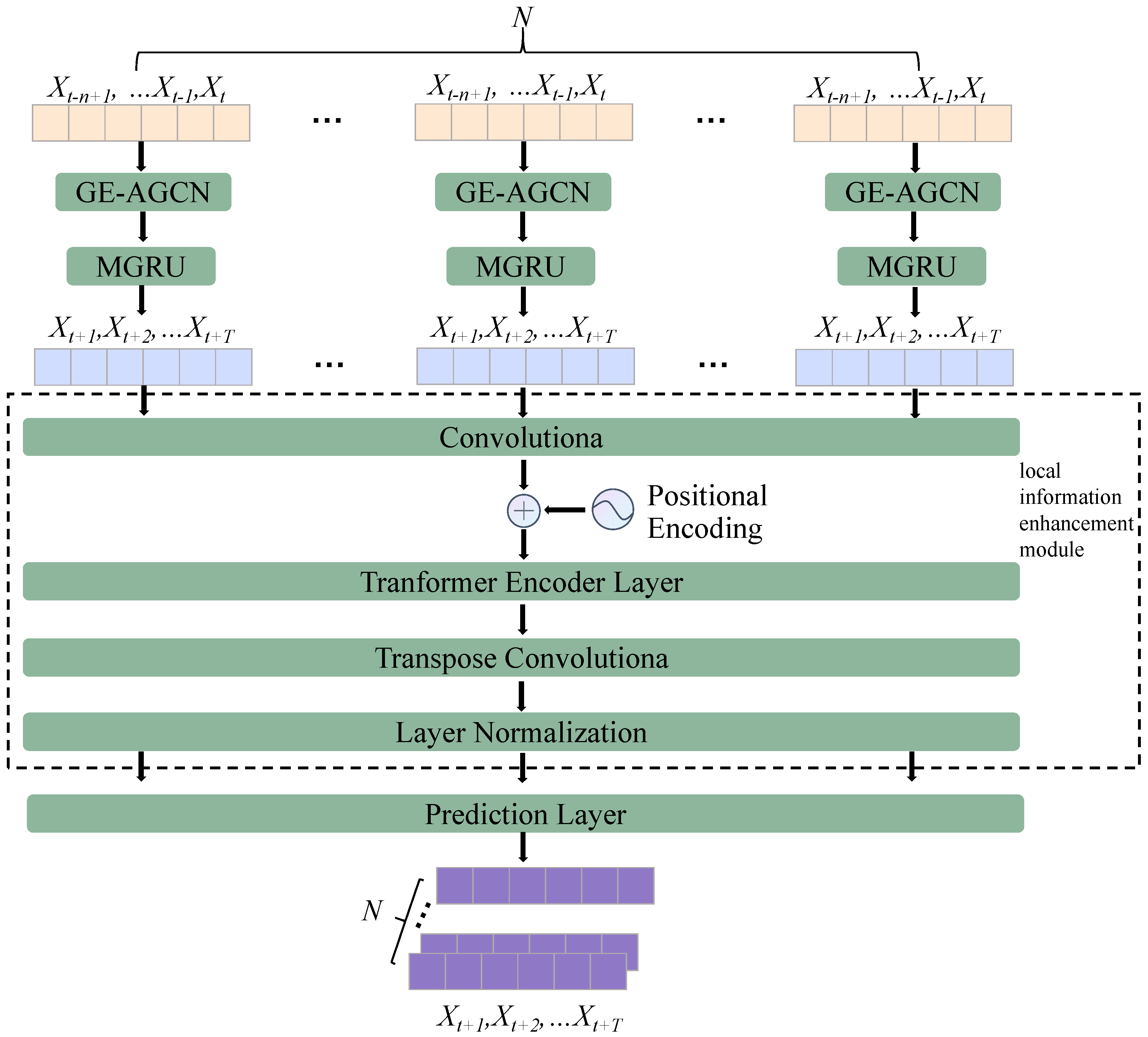
The EIGRN is composed of three parts: a GE-AGCN, an MGRU, and a local information enhancement module. The GE-AGCN learns the relevant information of the topology graph through graph embedding, generates an adaptive matrix instead of the original topology graph to capture the spatial information of each node, and learns the specific parameters for each node. Compared to a GRU, the MGRU ’s hidden layer unit, ht, passes through the spatial model GE-AGCN, thereby strengthening the learning of spatial information while capturing the time correlation. The local information enhancement module is used to simultaneously learn the global and local correlations of the data. It consists of a CNN, a transposed convolutional neural network, and a Transformer encoder layer. The Transformer encoder layer is made up of an attention mechanism and a feed-forward neural network. The attention mechanism is used to capture the global correlation of the data, whereas the CNN is used to capture the local context information of the data. They combine to make up for the limitations of the local imperceptibility of the attention mechanism. To capture different local information, multiple local information enhancement units are arranged in series in this model. As shown in Figure 2, the historical traffic data of length n are inputted into the model. The data are entered into the GE-AGCN, which learns the hidden spatial information of the data and then inputs this information into the MGRU. The MGRU strengthens the capturing of the spatial correlation while learning the temporal correlation. Finally, the obtained temporal sequences with spatio-temporal correlations are input into the local information enhancement module to capture the global and local correlations of the data. At the same time, in order to avoid the vanishing gradients problem, residual connections [25] are used to connect the outputs.

3.3. Methodology

3.3.1. Modeling the Spatial Correlation

A GCN is adopted to transform and disseminate information in the data. The traditional formula of the GCN is as follows:

$$X_{out}=(I_N+D^{-1/2}A{D}^{-1/2})X_{in}·W+b$$

(2)

where W and b represent the parameters for learning, $X_{in}\in R^{N\times d_{in}}$ represents the historical traffic data, and $X_{out}\in R^{N\times d_{out}}$ represents the output after the GCN operation. $I_N$ represents the N-dimensional identity matrix, A represents the adjacent matrix of the traffic graph, and D represents the degree matrix.

In Formula (2), the operation is solely based on the road connection information of the traffic graph. However, in most cases, the spatial correlation is not fully captured. The adjacency topology of the road does not contain complete information about the spatial correlation and has no direct relationship with the forecasting task, which may result in considerable deviation. Meanwhile, through Formula (2), we find that all nodes share the same parameters W and b. However, the patterns of each node are not exactly the same. Although sharing the same parameters can reduce the number of parameters and learn the most prominent patterns in each node, ignoring the patterns of the other nodes is not desirable. Certain properties of two adjacent nodes such as the POI may differ and two adjacent nodes may present different or even completely opposite patterns. Therefore, it is insufficient to capture the shared patterns between all nodes so we allocate a parameter space for each node to learn node-specific patterns.

To address this issue, the GE-AGCN was proposed to automatically infer the hidden interdependencies from the data and learn the specific parameters of each node. Firstly, the GE-AGCN uses graph embedding to initialize the embedding dictionary using topological graph information. Graph embedding maps the nodes or edges of a graph to a low-dimensional vector space, representing high-dimensional complex and dynamic data as low-dimensional and dense vectors, which preserves the structure and properties of the graph. Node2vec [26] was used in this experiment.

The Node2vec algorithm is shown in Figure 3. Node2vec is one of the algorithms used for graph embedding. Based on the idea of text representation, it uses the random-walk strategy to sample vertices and generates the neighbor sequence of vertices. The Skip-gram model is then used to learn the vertex representation [27]. Unlike the uniform random-walk strategy utilized in DeepWalk [28], the Node2vec random-walk strategy incorporates bias. In addition, it introduces jump hyperparameters p and q to control the random-walk strategy. Assuming the current random walk has traversed edge (t,v) to vertex v, the transition probability from vertex v to vertex x is denoted as ${\pi }_{vx}={\alpha }_{pq}(t,x)·w_{vx}$, where $w_{vx}$ represents the weight of edges.

$${\alpha }_{pq}(t,x)=\left\{\begin{array}{c}\frac{1}{p},if{d}_{tx}=0\hfill \\ 1,if{d}_{tx}=1\hfill \\ \frac{1}{q},if{d}_{tx}=2\hfill \end{array}\right.$$

(3)

where $d_{tx}$ represents the shortest path between vertex t and vertex x, and the vertex transition probability is as follows:

$$P(c_i=x|c_{i-1}=v)=\left\{\begin{array}{c}\frac{{\pi }_{vx}}{Z},if(v,x)\in E\hfill \\ 0,otherwise\hfill \end{array}\right.$$

(4)

where ${\pi }_{vx}$ represents the transition probability between vertex v and vertex x, and Z represents the normalization constant. Node2vec learns the optimal hyperparameters p and q through the semi-supervised network, achieving the best balance between breadth-first and depth-first approaches and ensuring that the incorporation of both local and global network information from the network is balanced.

$E_A\in R^{N\times d}$ is generated using Node2vec, where each row of $E_A$ represents the embedding of a node, and d represents the dimension of node embedding. By multiplying $E_A$ and $E_A^T$, similar to defining the graph based on node similarity, we can infer the spatial dependencies between each pair of nodes.

$$D^{-1/2}A{D}^{-1/2}=softmax\left(ReLU(E_A·E_A^T)\right)$$

(5)

where the $softmax$ function is used to normalize the adaptive matrix, and $D^{-1/2}A{D}^{-1/2}$ is directly generated to avoid unnecessary computations in the training process. In the training process, $E_A$ automatically updates to learn the hidden relationship between different traffic sequences and obtain the adaptive matrix of graph convolution. So, the GCN formula can be formulated as Formula (6):

$$X_{out}=(I_N+softmax\left(ReLU(E_A·E_A^T)\right))X_{in}·W+b$$

(6)

Next, the specific parameters for each node are learned by adopting the idea of matrix decomposition to improve the parameters W and b. A randomized weight pool, denoted as $W_G\in R^{d\times C\times F}$, is constructed. We set $d<<N$, which can significantly reduce the number of parameters and speed up the operation of the model. Then, W can be generated through $W=E_A·W_G$, with $E_A$ and $W_G$ continuously updated during training to learn each node-specific pattern. b can also be generated using the same operation. Finally, the GCN formula can be expressed as Formula (7):

$$\begin{array}{cc}\hfill & X_{out}=(I_N+softmax\left(ReLU(E_A·E_A^T)\right))X_{in}·E_A·W_G+E_A·b_G\hfill \end{array}$$

(7)

By using the above method, we can address the limitations of traditional GCNs, which are highly dependent on the topological graph and share the same parameters. Moreover, this method enables us to discover deeper hidden relationships among the nodes.

3.3.2. Modeling the Temporal Correlation

The most commonly used method for capturing the temporal correlation of data is the RNN. However, the long-term forecasting performance of traditional RNNs is poor [29]. The LSTM and GRU models, which are variations of the RNN, use gated mechanisms to preserve long-term information, resulting in accurate results in long-term forecasting. However, the GRU model is simpler and faster than the LSTM model. Therefore, the GRU model is used to capture the time correlation of the data.

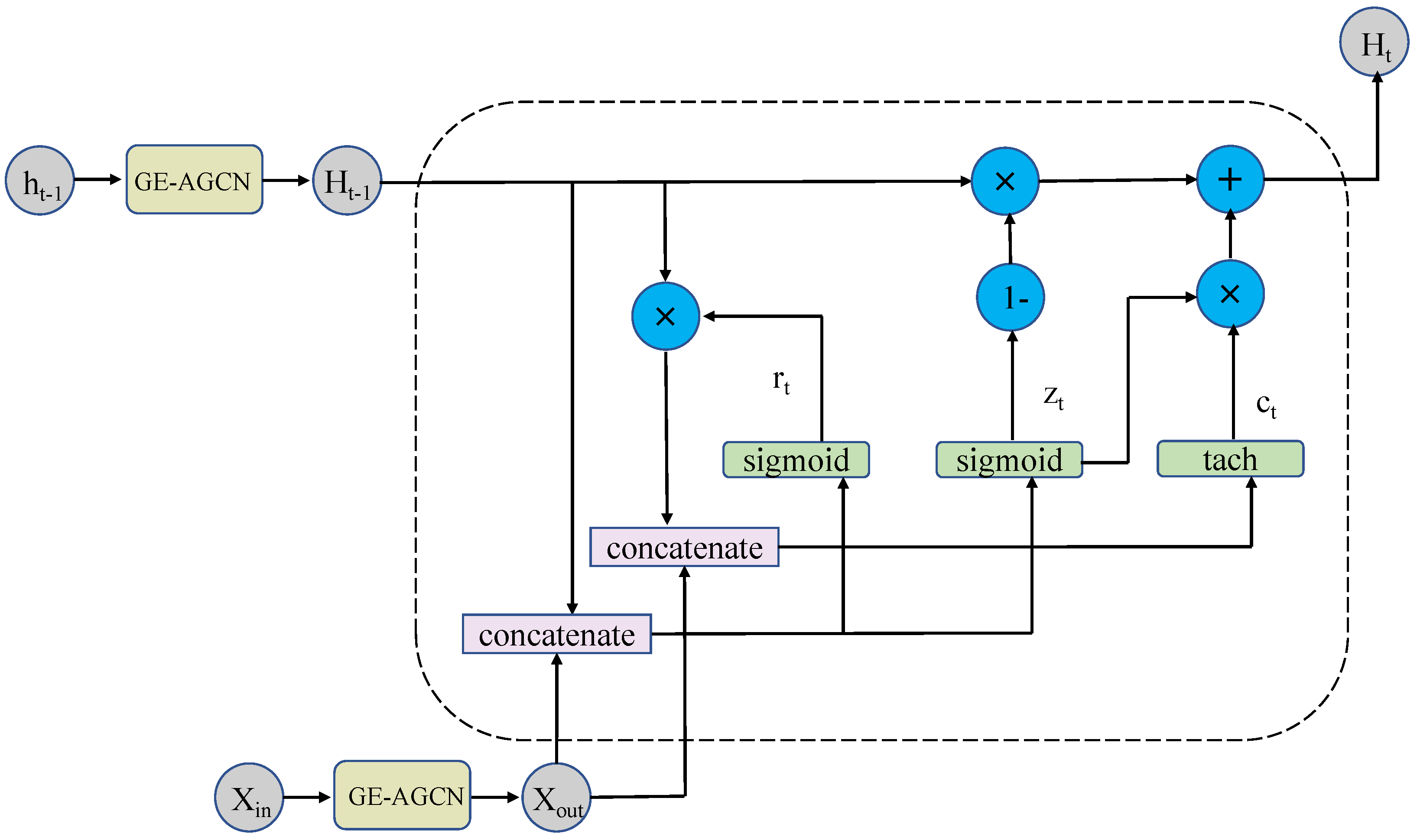
The GRU uses the hidden state of time $t-1$ and the current traffic information as input to obtain the traffic information at time t. As shown in Figure 4, $r_t$ is the reset gate, which controls the extent to which the state information from the previous moment is disregarded; $u_t$ is the update gate, which controls the incorporation of the state information from the previous moment into the current state; $c_t$ is the memory content stored at time t time; and $h_{t-1}$ is the hidden state at time $t-1$. In order to capture temporal information and incorporate spatial relationships, we applied an improved GCN operation on the hidden layer unit of the GRU. Specifically, in the original GRU, $h_t$ is fed directly into the GRU; however, in our approach, $h_t$ first enters the GE-AGCN before being fed into the GRU. Compared to a traditional GRU, our approach allows $h_t$ to capture the spatial correlation of traffic data, which enables the model to capture both the spatial and temporal information of the data. This means that the MGRU can transform the hidden state $h_{t-1}$ of a traditional GRU at moment t into a new hidden state $H_{t-1}$, which contains the current spatial information through the use of the GE-AGCN, as shown in Formula (8):

$$\begin{array}{cc}\hfill & H_{t-1}=(I_N+softmax\left(ReLU(E_A·E_A^T)\right))h_{t-1}·E_A·W_G+E_A·b_G\hfill \end{array}$$

(8)

The modified GRU formula is shown in Formulas (9)–(12):

$$u_t=\sigma (W_u[X_{out},H_{t-1}]+b_u)$$

(9)

$$r_t=\sigma (W_r[X_{out},H_{t-1}]+b_r)$$

(10)

$$c_t=\sigma (W_c[X_{out},(r_t\times H_{t-1})]+b_c)$$

(11)

$$H_t=u_t\times H_{t-1}+(1-u_t)\times c_t$$

(12)

$X_{out}$ represents the output of the modified GCN and is defined in Formula (7). W and b are two learnable parameters that represent the weights and biases in the training process. As shown in Formula (12), at moment t the current hidden state $H_t$, which contains the spatial information, can be obtained using the MGRU.

3.3.3. Global and Local Correlations

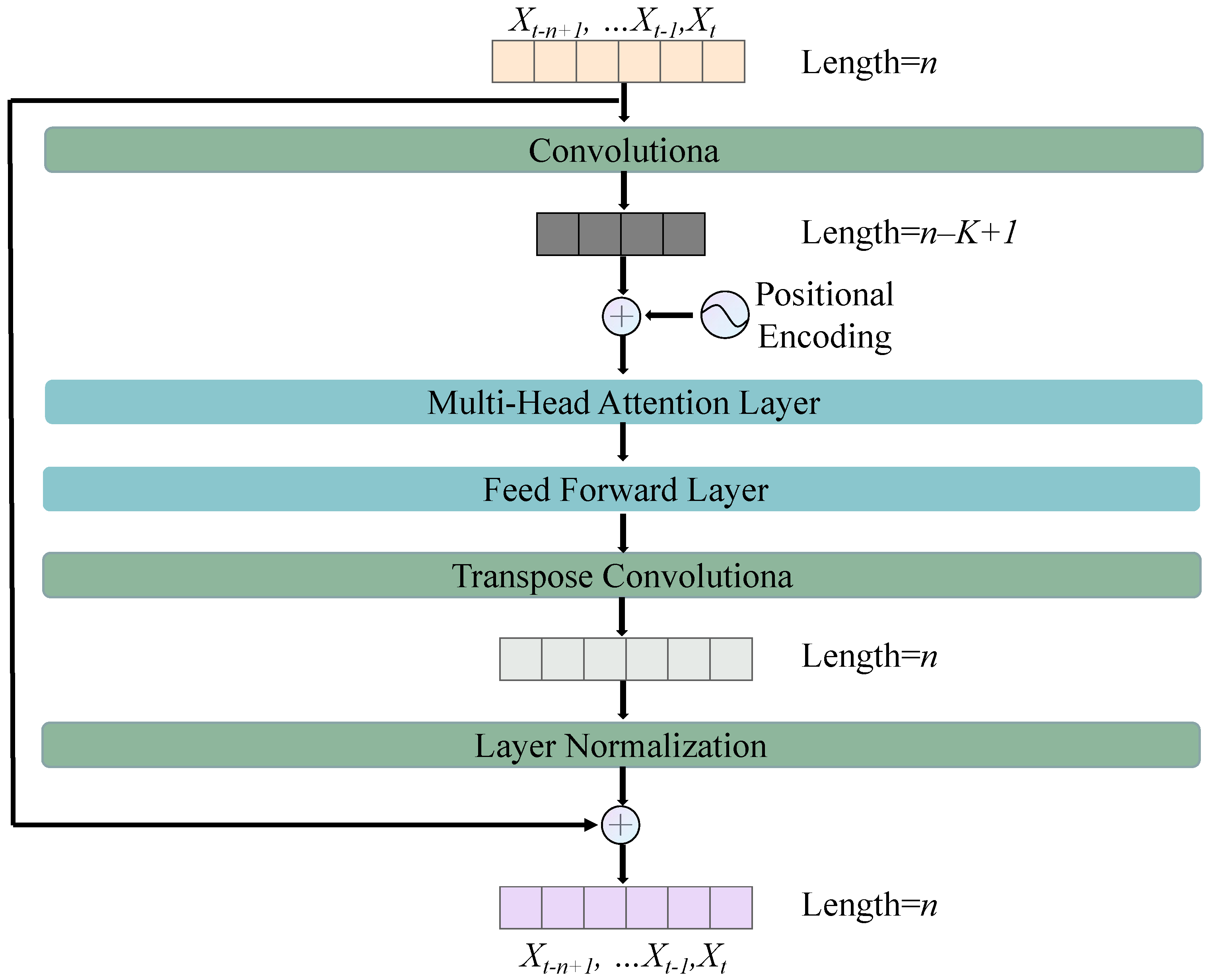
Each local information enhancement module consists of a CNN with a convolution kernel size of K, a transposed convolutional neural network with a convolution kernel size of K, and an attention mechanism. The framework of our local information enhancement module is shown in Figure 5. First, the traffic data is fed into the CNN with a convolution kernel with a width of K. The CNN searches for K neighboring elements of the input, and the padding is set to 0 in this experiment, which maintains the length of each sequence as $K-1$. The data processed by the CNN are then passed into the multiple attention layer [18]. The multiple attention layer is based on the dot-product attention mechanism. In the multiple attention layer, each element at sequence position i is related to all the elements in the sequence. The inputs of the attention function consist of queries and keys with dimension $d_k$ and values with dimension $d_v$ of all the positions in the sequence. By calculating the attention score for each position and using it as the weight, the traditional attention can be computed, as shown in Formula (13):

$$Attention(Q,K,V)=softmax\left(\frac{Q{K}^T}{\sqrt{d_k}}V\right)$$

(13)

$Q,K\in R^{T\times d_k}$ and $V\in R^{T\times d_v}$ denote the queries, keys, and values for all the nodes. The i-th row of Q represents the query for position i in the sequence. Multi-head attention allows the model to simultaneously focus on information from different representative subspaces at different locations. In contrast, when using a single attention head, the averaging process hinders this ability. Therefore, multi-head attention is more effective. The equation for multi-head attention is shown in Formula (14):

$$MultiHead(Q,K,V)=Concat(hea{d}_1,\cdots hea{d}_h)W^O$$

(14)

where h is the number of heads. The equation for $hea{d}_i$ is shown in Formula (15):

$$hea{d}_i=Attention(Q{W}_i^Q,K{W}_i^K,V{W}_i^V)$$

(15)

$d_{model}$ represents the input dimension in $W_i^Q\in R^{d_{model}\times d_k}$, $W_i^K\in R^{d_{model}\times d_k}$, $W_i^V\in R^{d_{model}\times d_k}$, and $W^O\in R^{h{d}_v\times d_{model}}$. However, the multi-head attention layer ignores the relative positions in the sequence because it treats different positions equally when computing the attention function. To ensure that the multi-head attention layer captures the relative position of position i in the whole sequence, each position is encoded with $e_t$, where $e_t$ is defined in Formula (16):

$$e_t=\left\{\begin{array}{c}sin(t/10,{000}^{2i/d_{model}}),ift=0,2,4...\hfill \\ cos(t/10,{000}^{2i/d_{model}}),otherwise\hfill \end{array}\right.$$

(16)

The output of the multi-head attention layer is transmitted to the feed-forward neural network layer. Then, the data are fed into the transposed convolutional neural network with a convolution kernel with a width of K. Similarly, the transposed convolutional neural network searches for K adjacent elements of the input elements without padding, resulting in an increase in the length of each sequence by $K-1$. As shown in Figure 5, after the transposed convolutional neural network, a normalization layer is used [30]. Together, these components comprise the local information enhancement module.

To collect information from different local units, several local information enhancement modules are employed. Each module utilizes a different convolution kernel size. Due to the different convolution kernel sizes, the obtained receptive fields are also different so different local information can be captured. In general, the larger the kernel, the larger the field of perception, which allows for the acquisition of more information and better characterization of global features. However, too large a convolution kernel leads to an increase in the parameters, which is not conducive to increasing the depth of the model, as well as computational power. To account for the data dimension in this experiment, we use seven local information enhancement modules with convolution kernel sizes of 13, 11, 9, 7, 5, 3, and 1, respectively. Additionally, to better enable the model to learn information from the data and avoid gradient problems caused by deep layers, the residual connections are set at the end of the module.

The EIGRN model is capable of handling complex spatio-temporal data. The GE-AGCN can better capture spatial information by learning location representations. The MGRU can capture the dynamic temporal correlation in the traffic volume on the road. The local information enhancement module improves the ability to capture local spatio-temporal information while capturing the global correlation using a combination of a CNN and an attention mechanism.

4. Experiments

4.1. Data Description

We evaluated the effect of the model on two real datasets, the PEMS-BAY dataset and the PeMSD7(M) dataset. Both datasets are related to traffic speed.

(1) PEMS-BAY: This dataset contains traffic speed data collected by 325 traffic sensors in the California Bay area over 6 months. The dataset consists of two parts, namely the adjacency matrix corresponding to the road topology and the collected traffic speed data. The granularity of traffic speed data is 5 min.

(2) PeMSD7(M): This dataset contains traffic speed data collected by 228 sensors on California highways on workdays between May and June 2012. The dataset consists of an adjacency matrix and traffic speed data. The granularity of traffic speed data is 5 min.

In the experiments, the data were processed using Z-Score, and 70% of the data was used as the training set, 10% was used as the validation set, and 20% was used as the testing set.

4.2. Evaluation Metrics

We used two metrics to evaluate the forecasting performance of the model:

(1) Root Mean Squared Error (RMSE):

$$RMSE=\sqrt{\frac{1}{MN}\sum _{j=1}^M\sum _{i=1}^N{(y_i^j-{\widehat{y}}_i^j)}^2}$$

(17)

(2) Mean Absolute Error (MAE):

$$MAE=\frac{1}{MN}\sum _{j=1}^M\sum _{i=1}^N\left|(y_i^j-{\widehat{y}}_i^j)\right|$$

(18)

where $y_i^j$ and ${\widehat{y}}_i^j$ represent the real traffic information and the predicted information of the jth time samples in the ith road. M is the number of time samples; N is the number of roads; Y and $\widehat{Y}$ represent the sets $y_i^j$ and $\widehat{y_i^j}$, respectively; and $\overline{Y}$ is the average of Y.

Specifically, the RMSE and MAE are used to measure forecasting errors, where the smaller the value, the better the forecasting performance.

4.3. Hyperparameters

The hyperparameters of the model included the learning rate, batch size, number of local information enhancement modules, and embedding dimension. In the experiment, we set the learning rate to 0.003, the batch size to 64, the number of local information enhancement modules to 7, and the embedding dimension to 10.

Baseline Methods

To verify the validity of this model, it was compared with traditional and representative methods.

(1)

History Average (HA) model [31]: This model uses the average traffic information of the historical period for forecasting.

(2)

ARIMA [3]: Parameter model fitting of the observation time series is carried out to predict future traffic data.

(3)

Fully-connected LSTM (FC-LSTM) [32]: An RNN with fully connected LSTM hidden units.

(4)

STGCN [33]: The spatio-temporal graph convolution network integrates graph convolution into a one-dimensional convolution unit.

(5)

DRCNN [14]: This model combines a GCN with recursive units controlled by an encoder–decoder gate.

(6)

Graph WaveNet [15]: This model combines an adaptive adjacency matrix GCN with causal convolution.

(7)

STSGCN [34]: The STSGCN captures localized correlations independently by using localized spatial-temporal subgraph modules.

(8)

STTN [35]: The STNN dynamically captures spatio-temporal dependence using a Transformer model.

4.4. Experimental Results

Table 2. Forecasting results on the PEMS-BAY and PeMSD7(M) datasets.

Model	PEMS-BAY (15/30/60 min)		PeMSD7(M) (15/30/60 min)
	MAE	RMSE	MAE	RMSE
HA	2.88	5.59	4.01	7.20
ARIMA	1.62/2.33/3.38	3.30/4.76/6.50	5.55/5.86/6.27	9.00/9.13/9.38
FC-LSTM	2.05/2.20/2.37	4.19/4.55/4.96	3.57/3.92/4.16	6.20/7.03/7.51
DCRNN	1.38/1.74/2.07	2.95/3.97/4.74	2.25/2.98/3.83	4.04/5.58/7.19
STGCN	1.39/1.84/2.42	2.92/4.12/5.33	2.24/3.02/4.01	4.07/5.70/7.55
Graph WaveNet	1.30/1.63/1.95	2.73/3.67/4.63	2.14/2.80/3.19	4.01/5.48/6.25
STSGCN	2.54/2.60/2.71	4.79/4.93/5.28	1.99/2.43/3.04	3.59/4.63/6.01
STTN	1.36/1.67/1.95	2.87/3.79/4.50	2.14/2.70/*	4.04/5.37/*
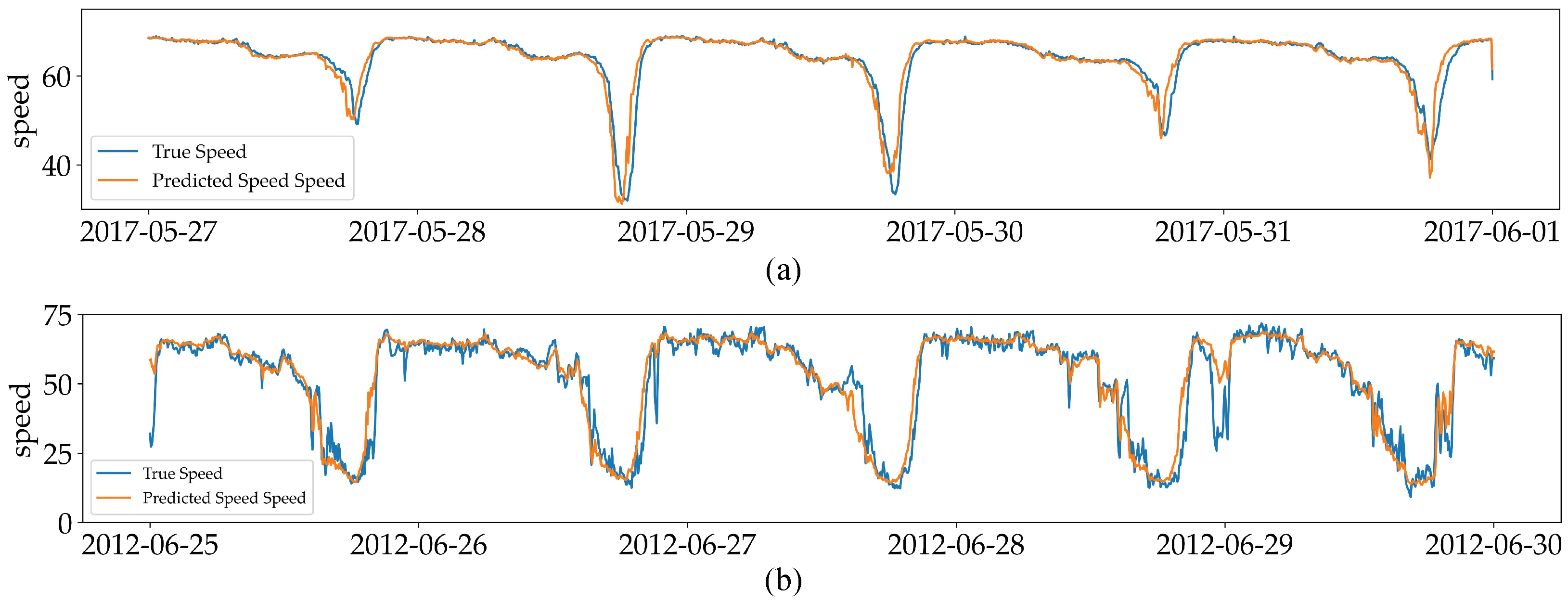
EIGRN	1.14/1.43/1.81	2.45/3.22/4.21	1.75/2.26/2.91	3.30/4.38/5.75

shows the MAE and RMSE of the EIGRN and the baselines for different period steps on the PEMS-BAY and PeMSD7(M) datasets. The results of the EIGRN demonstrate its good predictive ability. * indicates that the prediction error and the actual gap is large, so ignored. Moreover, the EIGRN successfully balanced the short-term and long-term predictions and achieved the best performance in almost all ranges. In order to more clearly demonstrate the effectiveness of our model, we visualized the prediction results of all the deep learning methods, as seen in Figure 6 and Figure 7. Additionally, Figure 8 shows the fitting effect of our model on the real and predicted values of the two datasets. From Table 2 we can see that the forecasting performance of the HA, ARIMA, and FC-LSTM methods was not good because these time series models can only capture the time information of the data, and it is difficult to improve the forecasting accuracy when the spatial information cannot be captured. The spatio-temporal models discussed below can address the above challenges to some extent. The forecasting performance of a model can be greatly improved if the spatial information of the data has been captured. In the generated graph models, the forecasting performance of Graph WaveNet was the best. In addition, the STSGCN, which is based on spatio-temporal synchronization forecasting, and the STTN, which is based on Transformer, also demonstrated good performance. In summary, the spatio-temporal models outperformed the temporal models, including the HA, ARIMA, and FC-LSTM models, by a large margin. This proves the effectiveness of spatio-temporal dependency modeling. Compared to other spatio-temporal models, the EIGRN significantly outperformed the STGCN and surpassed graph-generating-based approaches such as the DCRNN and Graph WaveNet. Our graph generated using graph embedding also achieved better results. Moreover, the EIGRN outperformed the spatio-temporal synchronization forecasting-based approaches such as the STSGCN and surpassed the Transformer approaches such as the STTN. This demonstrates that our model has better spatio-temporal forecasting ability.

Table 3. Forecasting iterations on the PEMS-BAY and PeMSD7(M) datasets.

Dataset	Average Training Time (Epoch)
	15 min	30 min	60 min
PEMSBAY	238	298	121
PeMSD7(M)	129	98	54

shows the number of training iterations for our two datasets. Figure 9 shows the loss changes of the two datasets. For our experiments, we selected the MAE as the loss function.

4.5. Ablation Studies

Three ablation experiments were designed to verify the effectiveness of our module. In EIGRN-G, the spatial model in the EIGRN was replaced with an ordinary GCN. In EIGRN-R, the improved GRU in the EIGRN was removed. In EIGRN-T, the local information enhancement module in the EIGRN was removed. The results of the ablation experiments are shown in

Table 4. Forecasting results on the PEMS-BAY and PeMSD7(M) datasets.

Model	PEMS-BAY (15/30/60 min)		PeMSD7(M) (15/30/60 min)
	MAE	RMSE	MAE	RMSE
EIGRN	1.14/1.43/1.81	2.45/3.22/4.21	1.75/2.26/2.91	3.30/4.38/5.75
EIGRN-T	1.14/1.43/1.86	2.49/3.28/4.26	1.76/2.29/2.98	3.31/4.45/5.84
EIGRN-R	1.15/1.44/1.86	2.43/3.26/4.21	1.76/2.27/2.96	3.33/4.44/5.88
EIGRN-G	2.16/2.26/2.44	4.44/4.62/5.14	3.81/3.83/4.11	7.47/7.50/7.85

and the visualization results are shown in Figure 10 and Figure 11. Regarding the forecasting performance of the EIGRN-G model, we can see that when our spatial model was replaced with the original GCN, the RMSE and MAE errors increased across all periods. This indicates that our graph embedding-based generative graph model had better spatial forecasting ability, thereby proving the effectiveness of our spatial model. In addition, the forecasting results of the EIGRN-R and EIGRN-T exhibited similar patterns. This demonstrates that the time-capturing ability of the MGRU improved after capturing spatial information. In addition, the local information enhancement module captured the importance of global and local relationships.

Accurate prediction of traffic speed can help traffic management departments monitor traffic congestion more effectively and implement appropriate traffic control measures. It also enables traffic management departments and drivers to take necessary actions such as adjusting speed limits to reduce accidents and improve road safety.

5. Conclusions

A modified traffic volume forecasting model called the EIGRN is proposed in this paper. By using this model, both the spatio-temporal correlations and the global and local correlations of the traffic data can be captured simultaneously and more effectively. As a result, the prediction ability of the model for traffic data is improved. Specifically, a GE-AGCN is used to capture the spatial correlation of traffic data by using graph embedding to generate an adaptive matrix. An MGRU is used to capture the temporal correlation by using gated mechanisms. A local information enhancement unit captures the global and local information of the data by combining a CNN with different convolution kernels and attention mechanisms. The presented method is tested on two real traffic datasets and compared with the HA, ARIMA, FC-LSTM, DCRNN, STGCN, Graph Wavenet, STSGCN, and STTN models. The experimental results demonstrate that the proposed EIGRN model outperforms the comparison models across various forecasting levels.

References

1. Jian, Y.; Bingquan, F. Synthesis of short-term traffic flow forecasting research progress. Urban Transp. China 2012, 10, 73–79. [Google Scholar]
2. Ahmed, M.S.; Cook, A.R. Analysis of freeway traffic time-series data by using Box-Jenkins techniques. Transp. Res. Rec. 1979, 722, 1–9. [Google Scholar]
3. Hamed, M.M.; Al-Masaeid, H.R.; Said, Z.M.B. Short-term prediction of traffic volume in urban arterials. J. Transp. Eng. 1995, 121, 249–254. [Google Scholar] [CrossRef]
4. Okutani, I.; Stephanedes, Y.J. Dynamic prediction of traffic volume through Kalman filtering theory. Transp. Res. Part B Methodol. 1984, 18, 1–11. [Google Scholar] [CrossRef]
5. Wu, C.H.; Ho, J.M.; Lee, D.T. Travel-time prediction with support vector regression. IEEE Trans. Intell. Transp. Syst. 2004, 5, 276–281. [Google Scholar] [CrossRef] [Green Version]
6. Yao, Z.s.; Shao, C.f.; Gao, Y.l. Research on methods of short-term traffic forecasting based on support vector regression. J. Beijing Jiaotong Univ. 2006, 30, 19–22. [Google Scholar]
7. Sun, S.; Zhang, C.; Yu, G. A Bayesian network approach to traffic flow forecasting. IEEE Trans. Intell. Transp. Syst. 2006, 7, 124–132. [Google Scholar] [CrossRef]
8. Shi, X.; Chen, Z.; Wang, H.; Yeung, D.Y.; Wong, W.K.; Woo, W.C. Convolutional LSTM network: A machine learning approach for precipitation nowcasting. Adv. Neural Inf. Process. Syst. 2015, 28, 802–810. [Google Scholar]
9. Zhang, J.; Zheng, Y.; Qi, D. Deep spatio-temporal residual networks for citywide crowd flows prediction. In Proceedings of the Thirty-First AAAI Conference on Artificial Intelligence, San Francisco, CA, USA, 4–9 February 2017. [Google Scholar]
10. Zhang, H.; Chen, L.; Cao, J.; Zhang, X.; Kan, S. A combined traffic flow forecasting model based on graph convolutional network and attention mechanism. Int. J. Mod. Phys. C 2021, 32, 2150158. [Google Scholar] [CrossRef]
11. Ye, J.; Zhao, J.; Ye, K.; Xu, C. How to build a graph-based deep learning architecture in traffic domain: A survey. IEEE Trans. Intell. Transp. Syst. 2020, 23, 3904–3924. [Google Scholar] [CrossRef]
12. Yin, X.; Wu, G.; Wei, J.; Shen, Y.; Qi, H.; Yin, B. A comprehensive survey on traffic prediction. arXiv 2020, arXiv:2004.08555. [Google Scholar]
13. Zhao, L.; Song, Y.; Zhang, C.; Liu, Y.; Wang, P.; Lin, T.; Deng, M.; Li, H. T-gcn: A temporal graph convolutional network for traffic prediction. IEEE Trans. Intell. Transp. Syst. 2019, 21, 3848–3858. [Google Scholar] [CrossRef] [Green Version]
14. Li, Y.; Yu, R.; Shahabi, C.; Liu, Y. Diffusion convolutional recurrent neural network: Data-driven traffic forecasting. arXiv 2017, arXiv:1707.01926. [Google Scholar]
15. Wu, Z.; Pan, S.; Long, G.; Jiang, J.; Zhang, C. Graph wavenet for deep spatial-temporal graph modeling. arXiv 2019, arXiv:1906.00121. [Google Scholar]
16. Bai, L.; Yao, L.; Li, C.; Wang, X.; Wang, C. Adaptive graph convolutional recurrent network for traffic forecasting. Adv. Neural Inf. Process. Syst. 2020, 33, 17804–17815. [Google Scholar]
17. Li, M.; Zhu, Z. Spatial-temporal fusion graph neural networks for traffic flow forecasting. In Proceedings of the AAAI Conference on Artificial Intelligence, Vancouver, BC, Canada, 2–9 February 2021; Volume 35, pp. 4189–4196. [Google Scholar]
18. Vaswani, A.; Shazeer, N.; Parmar, N.; Uszkoreit, J.; Jones, L.; Gomez, A.N.; Kaiser, Ł.; Polosukhin, I. Attention is all you need. Adv. Neural Inf. Process. Syst. 2017, 30, 5998–6008. [Google Scholar]
19. Zhang, S.; Guo, Y.; Zhao, P.; Zheng, C.; Chen, X. A graph-based temporal attention framework for multi-sensor traffic flow forecasting. IEEE Trans. Intell. Transp. Syst. 2021, 23, 7743–7758. [Google Scholar] [CrossRef]
20. An, J.; Guo, L.; Liu, W.; Fu, Z.; Ren, P.; Liu, X.; Li, T. IGAGCN: Information geometry and attention-based spatiotemporal graph convolutional networks for traffic flow prediction. Neural Netw. 2021, 143, 355–367. [Google Scholar] [CrossRef]
21. Wang, X.; Ma, Y.; Wang, Y.; Jin, W.; Wang, X.; Tang, J.; Jia, C.; Yu, J. Traffic flow prediction via spatial temporal graph neural network. In Proceedings of the Web Conference 2020, Taipei, Taiwan, 20–24 April 2020; pp. 1082–1092. [Google Scholar]
22. Liao, L.; Hu, Z.; Zheng, Y.; Bi, S.; Zou, F.; Qiu, H.; Zhang, M. An improved dynamic Chebyshev graph convolution network for traffic flow prediction with spatial-temporal attention. Appl. Intell. 2022, 54, 16104–16116. [Google Scholar] [CrossRef]
23. Lan, S.; Ma, Y.; Huang, W.; Wang, W.; Yang, H.; Li, P. Dstagnn: Dynamic spatial-temporal aware graph neural network for traffic flow forecasting. In Proceedings of the International Conference on Machine Learning. PMLR, Baltimore, MD, USA, 17–23 July 2022; pp. 11906–11917. [Google Scholar]
24. Li, S.; Jin, X.; Xuan, Y.; Zhou, X.; Chen, W.; Wang, Y.X.; Yan, X. Enhancing the locality and breaking the memory bottleneck of transformer on time series forecasting. Adv. Neural Inf. Process. Syst. 2019, 32, 5243–5253. [Google Scholar]
25. He, K.; Zhang, X.; Ren, S.; Sun, J. Deep residual learning for image recognition. In Proceedings of the IEEE Conference on Computer Vision and Pattern Recognition, Las Vegas, NV, USA, 27–30 June 2016; pp. 770–778. [Google Scholar]
26. Grover, A.; Leskovec, J. node2vec: Scalable feature learning for networks. In Proceedings of the 22nd ACM SIGKDD International Conference on Knowledge Discovery and Data Mining, San Francisco, CA, USA, 13–17 August 2016; pp. 855–864. [Google Scholar]
27. Mikolov, T.; Sutskever, I.; Chen, K.; Corrado, G.S.; Dean, J. Distributed representations of words and phrases and their compositionality. Adv. Neural Inf. Process. Syst. 2013, 26, 3111–3119. [Google Scholar]
28. Lai, S.; Liu, K.; He, S.; Zhao, J. How to generate a good word embedding. IEEE Intell. Syst. 2016, 31, 5–14. [Google Scholar] [CrossRef]
29. Bengio, Y.; Simard, P.; Frasconi, P. Learning long-term dependencies with gradient descent is difficult. IEEE Trans. Neural Netw. 1994, 5, 157–166. [Google Scholar] [CrossRef] [PubMed]
30. Ba, J.L.; Kiros, J.R.; Hinton, G.E. Layer normalization. arXiv 2016, arXiv:1607.06450. [Google Scholar]
31. Liu, J.; Wei, G. A Summary of Traffic Flow Forecasting Methods. J. Highw. Transp. Res. Dev. 2004, 21, 82–85. [Google Scholar]
32. Sutskever, I.; Vinyals, O.; Le, Q.V. Sequence to sequence learning with neural networks. Adv. Neural Inf. Process. Syst. 2014, 27, 3104–3112. [Google Scholar]
33. Yu, B.; Yin, H.; Zhu, Z. Spatio-temporal graph convolutional networks: A deep learning framework for traffic forecasting. arXiv 2017, arXiv:1709.04875. [Google Scholar]
34. Song, C.; Lin, Y.; Guo, S.; Wan, H. Spatial-temporal synchronous graph convolutional networks: A new framework for spatial-temporal network data forecasting. In Proceedings of the AAAI Conference on Artificial Intelligence, New York, NY, USA, 7–8 February 2020; Volume 34, pp. 914–921. [Google Scholar]
35. Xu, M.; Dai, W.; Liu, C.; Gao, X.; Lin, W.; Qi, G.J.; Xiong, H. Spatial-temporal transformer networks for traffic flow forecasting. arXiv 2020, arXiv:2001.02908. [Google Scholar]
Figure 1. An example of the disadvantages of using an attention mechanism to capture data information. (a) Traffic speed of PeMSD7 (M) dataset road id 49 at 1:00 on 7 May 2012. (b) Traffic speed of PeMSD7 (M) dataset road id 49 at 0:55 on 9 May 2012. (c) the traffic speed of road id 49 on PeMSD7(M) dataset from 6 May 2012 to 11 May 2012.
Electronics 12 02519 g001
Figure 2. Framework of the proposed model.
Electronics 12 02519 g002
Figure 3. The Node2vec algorithm.
Electronics 12 02519 g003
Figure 4. The architecture of the MGRU model.
Electronics 12 02519 g004
Figure 5. Framework of the local information enhancement module.
Electronics 12 02519 g005
Figure 6. The prediction performance of the EIGRN on the PEMS-BAY dataset is compared with that of other deep learning models.
Electronics 12 02519 g006
Figure 7. The prediction performance of the EIGRN on the PeMSD7(M) dataset is compared with that of other deep learning models.
Electronics 12 02519 g007
Figure 8. (a) Visualization results of the predicted and real values of the PEMS-BAY dataset. (b) Visualization results of the predicted and real values of the PeMSD7(M) dataset.
Electronics 12 02519 g008
Figure 9. (a) Visualization loss of the PEMS-BAY dataset. (b) Visualization loss of the PeMSD7(M) dataset.
Electronics 12 02519 g009
Figure 10. The ablation results of the EIGRN on the PEMS-BAY dataset.
Electronics 12 02519 g010
Figure 11. The ablation results of the EIGRN on the PeMSD7(M) dataset.
Electronics 12 02519 g011