Abstract
Cyber deception technology plays an important role in monitoring attackers’ activities and detecting new attack types. However, in a deceptive environment, low-risk attack traffic, such as scanning, is included in large quantities and acts as noise. Therefore, even though high-risk traffic is actually present, it may be overlooked, or the analysis algorithm’s accuracy regarding traffic may be reduced, causing significant difficulties in intrusion detection and analysis processes. In this study, we propose a model that can identify and filter the ordinal scale risk of the source IP in deceptive environment-generated traffic. This model aims to quickly classify low-risk attacks, including information gathering and scanning, which are widely and repeatedly performed, as well as high-risk attacks, rather than classifying specific types of attacks. Most existing deceptive technology-based Cyber Threat Intelligence (CTI) generation studies have been limited in their applicability to real-world environments because data labeling, learning, and detection processes using AI algorithms that consume significant amounts of time and computing resources. Here, the Naive Bayes discriminant analysis-based ordinary scale classification model showed higher accuracy for low-risk attack classification, while consuming significantly fewer resources than the models presented in other studies do. The accuracy of the current active deceptive environment traffic analysis research may be enhanced by filtering low-risk traffic via preprocessing.
1. Introduction
Deception technology plays a significant role in generating Cyber Threat Intelligence (CTI) information for increasingly sophisticated attacks [1,2]. Those in both academia and industry are actively researching the use of deception technology, not only for the active detection of and defense against attacks, but also for creating effective CTI. CTI is an intelligence technology that has recently shown significant potential in the IT cyber security community for responding to new threats. Deception technology is used to generate CTI that can protect assets from threats posed by more sophisticated attackers. However, research on using deception technology for CTI generation is often costly and has limited accuracy. While serious threats may be included in the data collected in deceptive environments, distinguishing low-level attacks that are included in large numbers from actual threats can be difficult or require high-cost technologies, such as classification using AI algorithms.
In this study, the risk of sources accessing the deceptive environment is evaluated using Naive Bayes discriminant analysis to identify the ordinal scale. The proposed Naive Bayes discriminant analysis technique is applied to understand the characteristics of sources accessing the deceptive environment based on the distribution of attack sources. Then, each Naive Bayes probability model is developed to identify the risk based on the characteristics of the attack source distribution and define the ordinal scale. Furthermore, the goal is to filter out attack sources identified on the low ordinal scale and select real threat sources.
This study makes the following contributions:
- Provides the analysis and visibility of attack distributions to identify the characteristics of sources attacking deceptive environments.
- Maximizes the utilization of CTI by applying the risk level when CTI is created using deceptive technology.
- Improves deceptive data analysis accuracy by filtering large amounts of data on a low-risk ordinal scale, such as noise.
- Provides Naive-Bayes-based discriminant analysis for rapid risk assessment.
Section 2 introduces related work on deception technology and CTI. Section 3 presents our proposed model that uses discriminant analysis with a Naive Bayes algorithm. Section 4 shows the results of running the model and evaluates its performance. Section 5 discusses the limitations of the proposed model and suggestions for future work. Section 6 concludes this paper, summarizing its research results and contributions.
2. Related Work
In this section, we review the classification of attack types and CTI generation using data from deceptive environments.
2.1. Deceptive Technology
The deception technique, which was an essential military strategy [3,4], was first mentioned in the field of cybersecurity in 1989, when Stoll published the book The Cuckoo’s Egg [5]. Stoll explained a method of creating a virtual system with fake user accounts and files to lure and delay attackers. Afterward, he established a system and role for the classification and terminology of deception techniques and continued to define them [2,6]. In 2001, Spitzner named the virtual environment for attacker deception Honeypot [7]. In addition, Spitzner proposed Honeypot technology, which was used to detect and gather information about external threats, as a way to detect threats caused by insiders [7]. Spitzner later proposed the concept of the Honeytoken [8], which refers to all resources used to lure attackers, such as files, database entries, and network ports, and it was first defined and used by de Barros in 2007 [9].
Research on constructing more sophisticated Honeytokens to deceive attackers has also been actively conducted on various resource types, such as document files, databases, passwords, and URL parameters. In 2005, Cenys deployed a Honeytoken in the Oracle database to detect malicious behavior [10]. To make a HoneyGen database that attackers could not differentiate from the real world, Bercovitch proposed HoneyGen in 2011 [11]. In 2013, Jewel and Rivest proposed the Honey password to detect whether an attacker’s password had been cracked [12]. In 2015, Kaghazgaran utilized permissions as a feature for attack detection and named it Honey Permission [13]. Recently, there has been substantial research into employing AI algorithms to create fake documents [14]. In 2021, Karuna conducted a study to generate fake documents using genetic algorithms to confuse attackers [15], and in 2022, Taofeek proposed a cognitive deception model (CDM) to generate fake documents using neural network algorithms [16].
2.2. Cyber Threat Iitelligence
Threat Intelligence (TI) is evidence-based knowledge, including context, mechanisms, indicators, meanings, and actionable advice, that is used for determining how to respond to a threat or risk [17]. In addition, it consists of information collected from a variety of technical or human sources and should include actionable guides, such as technical indicators, mechanisms, and actions. As shown in Table 1, Tounsi and Rais (2018) categorized TI into four areas: strategic TI, operational TI, tactical TI, and technical TI [18].

Table 1.
Four sub-domains of Threat Intelligence (TI).
The TI to be addressed in this study is technical TI, which detects intrusion mainly through monitoring by Indicators of Compromise (IOCs). In 2015, Ray categorized IOCs into three types: network-based, email-based, and host-based ones [19]. Examples of each type can be found in Table 2.
Table 2.
Categorization of major IOCs.
2.3. CTI Refinement in Deception
The technology used to analyze attacks in a deceptive environment and generate CTI is being actively studied. Although it is certain that the source accessing the deceptive environment has malicious intentions, numerous techniques are used, many of which make use of machine learning and deep learning algorithms, to determine which attack vector was used or how risky it was.
In 2015, Redwood proposed a Honeynet framework that could be operated by SCADA called SCyPH and created CTI using an anomaly detection algorithm supported by ETSY Skyline [20]. The ensemble-based anomaly analysis of multiple algorithms aims to detect automated or sophisticated attacks by bots that pose a threat to SCADA. In 2019, Banerjee conducted a study to detect botnets by collecting logs and traffic generated by intrusions into Honeynet [21]. Banerjee detected botnet using algorithms, such as Decision Tree, Gradient Boosting, and Random Forest. In 2022, Kumar proposed an approach to categorizing the high and low risk of an attack being launched on deceptive environments [22]. Kumar classified the degree of aggression through an ensemble of the AdaBoost, Random Forest Classifier, Light Gradient-Boosting Machine (LGBM), and XGBoost algorithms. As they used a collection of abnormality detection techniques, the aforementioned three studies are highly accurate, and thus, advantageous. However, the problem with using ensemble approaches is that learning or prediction takes time.
In 2021, Dutta used deceptive technology to detect attacks on IoT vulnerabilities and generate CTI. Dutta applied the Naive Bayes supervised classifier to collected network data to detect potential threats spreading to IoT devices [23]. Dutta’s method also shows high accuracy, but it is a burdensome task in that continuous separate labeling work is required. Additionally, in 2021, Kashtalian conducted a study using unsupervised learning based on the K-means algorithm to cluster Honeynet data [24]. Table 3 compares CTI studies based on deception data.
Table 3.
Comparison of deceptive data-based Cyber Threat Intelligence (CTI) research using machine learning algorithm.
In 2016, Urias proposed a different approach [25]. Instead of collecting and analyzing the IP addresses and vectors gathered during the compromised environment attack process, only post-compromise information was collected and analyzed. The goal was to create CTI using only IOC related to the actual successful attackers. While this approach provides clear and useful information, it is somewhat disappointing that it cannot identify the IoC used at the stage of compromising the system. There have also been studies that have used different approaches from that of Urias, without using machine learning algorithms. Fraunholz proposed a model that defines several characteristics and relationships of attacker types in advance and classifies attacks by applying attack instances [26,27].
3. Proposed Model
This section details the proposed probability model aimed at filtering for attacks with a low risk of infringement that occur extensively, such as scanning and information gathering.
The proposed model operates based on the traffic collected in the deceptive environment. It is an algorithm that determines whether the traffic generated by the corresponding source IP is low or high risk by applying discriminant analysis to each source IP.
3.1. Notation
Table 4 shows the notation used throughout this paper.
Table 4.
Notation.
3.2. Probability Distributions
This probability model indexes and calculates two items with the aim of identifying and filtering low-risk traffic, such as spying and information gathering, and high-risk traffic for infringement purposes in traffic flows occurring in a deceptive environment. First, we quantify the number of flows to the attack target to measure the frequency at which a given source IP approaches the deception host IP. Second, we quantify the range of targets to measure the extent to which a given source IP approaches various host IPs. The probability is then computed and compared using a probability model in which the two indicators are combined. If the probability of the source IP being of a low risk is higher than that of it being of a high risk, the goal is to distinguish high risk infringing traffic by identifying and filtering the source IP as executing a low risk attack.
Model 1.
The probability that a given source accessing destination IP in flow is of a low-risk ordinal scale can be expressed by the following equation:
Proof of Model 1.
Flows originating from low-risk IPs are mostly repetitive and numerous, and they generally exhibit a tendency to randomly access targets. In this study, a Gaussian distribution is used to represent the randomness of low-risk IPs, and it has been observed in the studies of Durumeric and Moore that the distribution of probe flows, including scans, follows a Gaussian distribution [28,29]. In this Gaussian distribution, and are the mean and standard deviation, respectively, calculated using the number of destinations, , accessed by each source, , belonging to the entire flow set, . □
Model 2.
The probability that a given source accessing destination IP is categorized as being of a high-risk ordinal scale can be expressed by the following equation:
Proof of Model 2.
Flows originating from high-risk IPs often communicate with a limited set of targets, but substantially more frequently than other flows do. Therefore, the probability distribution of a specific source IP being a high-risk IP also reflects the number of destination IPs with whom it communicates and the number of flows it generates toward restricted targets. The given probability, , increases as the number of flows between the source IP, , and destination IP, , increases and decreases, respectively, as the size of the destination IP set, , increases. □
Lemma 1.
The probability that a given source IP is of a high-risk ordinal scale for a set of destination IPs accessed by s can be expressed as follows:
Proof of Lemma 1.
In this study, the range of deceptive hosts that a source IP accesses is measured by figuring out the probability distribution of the set of flows that come from that source IP. If we denote the set of flows originating from source IP as , then is a subset of the set of all flows, . In this case, since the flows that make up have independent characteristics, the Naive Bayes classification model can be applied, and the joint probability distribution function can be used, as shown in the following equation.
Low-risk source IPs typically randomly access a large number of destination IPs. Therefore, the probability distribution of a low-risk IP selecting a target can be expressed as in Equation (5), which decreases relatively slowly as the number of destination IPs increases.
The probability that the source IP in a given flow set is of a low-ordinal-scale risk can be modeled by combining the equations above, as shown in Equation (3). □
Lemma 2.
The probability that a given source IP is of a high-risk ordinal scale for the set of destination IPs it has accessed can be expressed as follows:
Proof of Lemma 2.
Most of the time, high-risk source IPs choose their destination IPs for a specific reason and tend to only access a small number of destination IPs. Therefore, the probability distribution of the selection of high-risk IPs as destination IPs can be modeled as shown in Equation (8), and it exhibits a sharp decrease in probability as the number of destination IPs increases.
With the same approach as Lemma 1, we can apply the Naive Bayes model and derive Equation (4). By substituting (5) into Equation (4), we obtain function (7) to calculate the probability of a given flow set having a high-ordinal-scale risk for its source IP.
□
To effectively use the proposed model, we suggest Algorithm 1, which is simple, yet effective. The algorithm consists of six steps and is easily computed based on discriminant analysis. For each source IP, the algorithm calculates the classification probability distribution obtained in the previous section, compares the ratio of the two probabilities with a specific constant, and identifies the ordinal scale.
| Algorithm 1: Classification Model for Source IP Ordinal Scale | |||
| Data: Deception Flows DeceptionFlows Result: Flag OrdinalScale | |||
| 1 | DeceptionSources = DeceptionFlows.getUniqueSources() | ||
| 2 | for in DeceptionSources: | ||
| 3 | OrdinalScale = high | ||
| 4 | = DeceptionFlows.getFlows() | ||
| 5 | Compute | ||
| 6 | Compute | ||
| 7 | if : | ||
| 8 | OrdinalScale = low | ||
| 9 | end | ||
| 10 | end | ||
4. Empirical Evaluation
In this section, we aim to verify the accuracy of the proposed model and evaluate its performance. The detection performance is verified by running the model proposed in Section 3 and calculating the detection result accuracy. Additionally, the execution time and resource consumption are monitored to assess the resource efficiency of the proposed model.
4.1. Dataset
To evaluate the model, we used data collected from running a deception environment for over 6 months. The data collection period used for verification was from 1 September 2022 to 28 February 2023, and a total of 70 virtual machines were used, which were allocated to 4778 destination IPs. Additionally, each honeypot operates vulnerable versions of services supporting protocols, such as HTTP, SMB, RDP, and SMB, which run on each honeypot. However, their detailed configurations are extensive, and thus, omitted. The number of source IPs accessed during this period was 4,414,372, and a total of 3,772,436,978 flows were recorded. To use the proposed model, we aggregated packets into sessions using the open-source program, Arkime [30].
For data verification, 20,037 IPs, corresponding to 0.5% of all source IPs, were extracted and labeled. In the case of labeling, according to Durumeric’s research, flows containing invalid packets accessed due to packets that failed to establish a session, scans for reconnaissance, and configuration errors were manually checked and classified as low risk [28].
4.2. Model Execution
4.2.1. Result Evaluation
When the model is run on the source IP labeled with the risk, the results can be confirmed by the confusion matrix in Table 5. Of the total 20,037 source IPs, 18,992 are actual low-risk IPs and 1045 are actual high-risk IPs, while 18,551 are classified as low-risk IPs and 1486 are classified as high-risk IPs using the model.
Table 5.
Confusion matrix for model execution results with C = 1.
The classification accuracy, precision, recall, false positive (FP) rate, and failure rate for the model execution result with C = 1 can be found in Table 6. Although the recall for correctly classifying actual low-risk IPs is 97.17%, which can be considered as sufficient for the goal of creating a high-purity CTI based on the filter, it is important to minimize the cases where actual high-risk IPs are incorrectly classified as low-risk IPs and are not used to create CTI. Therefore, the FP rate should be considered, and at C = 1, the FP rate is 9.19%, which cannot be considered as a low value.
Table 6.
Evaluation metrics for model execution results at C = 1.
Figure 1 shows the changes in accuracy, recall, and FP rate with respect to the variation of the coefficient C for ordinal scale classification. As the value of C decreases, it can be observed that the accuracy, recall, and FP rate decrease as well.

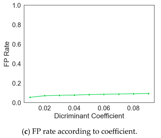
Figure 1.
Changes in evaluation index due to change in discriminant coefficient.
In this study, we aim to achieve maximum recall and minimum FP rates; so, we calculated the optimal coefficient using the difference between the recall and FP rate. Figure 2 shows that the optimal coefficient was achieved at C = 0.04, and Table 7 confirms that the recall was 95.74% and the FP rate was 7.56% at this point.

Figure 2.
Calculation of optimal value of coefficient C.
Table 7.
Evaluation metrics for model execution results at C = 0.04.
4.2.2. Distribution of Deceptive Environment Access from Source IP and Model Measurement
The probability distribution for the discriminant analysis proposed in this study was modeled by considering the concentration level of deceptive terminals targeted by the source IP and the level of flow generated. The degree to which this objective was achieved can be confirmed using the data in Figure 3. As the number of targets accessed by each source IP decreases and the number of flows generated increases, the trend of being identified as a high-risk IP can be observed.
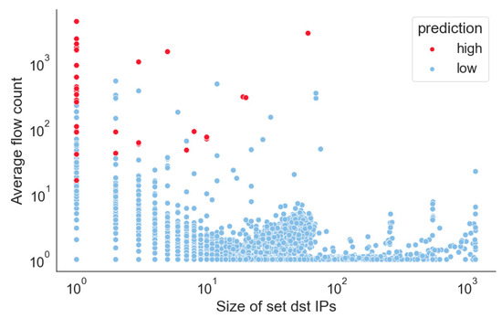
Figure 3.
Ordinal scale classification based on size of destination IP set accessed by source IP and average flow count.
When a model based on prior probability is used, such as a Bayes model, the cold start issue is always a problem that needs to be considered. When the initial or early sources that do not have enough prior data are judged, there may be problems with the results due to missing data before the starting point. The deception traffic used in this study has a greater impact as the connection period of these source IPs becomes longer. To confirm the degree of impact, we checked the connection period distribution of each source IP and found that it had an average connection period of 2 s. Therefore, an exception needs to be made for the initial 2 s in terms of the reliability of the IP classification results for the source IPs.
In addition, the Naive Bayes discriminant analysis was performed to estimate the behavior of the source IP from two different group perspectives, low and high ordinal scales, thereby minimizing the impact of time and environmental changes. The analysis results from the start date of the experimental data, 1 September 2022, to the middle date, 15 December 2022, to the end date, 28 February 2023, can be found in Figure 4 and Table 8.

Figure 4.
Distribution of connection times for deceptive environments of each source IP.
Table 8.
Evaluation metrics for model execution results at C = 0.04 on 1 September 2022, 15 December 2022, and 28 February 2023.
4.3. Performance Evaluation
Deceptive data generated in deceptive environments are often used in cybersecurity research; so, the performance of the preprocessing module must be considered. The prototype of the proposed model was written in Python, and 20 sets of hourly data were processed for the experiment to measure the time and resource consumption for each set. The experimental environment is shown in Table 9.
Table 9.
Hardware specifications of machine used to benchmark prototype.
The execution results were confirmed as shown in Table 10. Each set of hourly data was processed within an average of 5 min and 11 s, including the preprocessing step, and it was confirmed that the average CPU usage was 24.59%, and the average memory usage was 493 MB. The experimental environment was configured as a virtual machine, and considering that most of the CTI generation programs operate on the server, it can be confirmed that they are processed quickly using considerably fewer resources.
Table 10.
Performance measurement results.
5. Discussion
This study has some limitations, which are outlined in the section below.
5.1. Limitations
The model proposed in this study has two limitations. The first one is that it is dependent on the number of targets accessed by the source IP and the number of flows generated. For example, if a serious attack is executed in a way that generates the minimum number of flows for multiple targets, it can be difficult to distinguish it from a low-risk attack. Future research must identify and implement other characteristics that distinguish serious attacks from low-risk attacks. However, since this study aims to quickly and efficiently remove noise, new features should be easily obtainable or calculable, and the emphasis should be on minimizing their number. The second limitation is that while the proposed model can efficiently and quickly classify the ordinal scale of attack traffic collected in a deceptive environment, it is not suitable for classifying attack types in more detail or with greater granularity.
5.2. Future Work
In future research, additional feature engineering is needed to overcome the abovementioned limitations, such as distinguishing serious attacks from low-risk attacks that generate a minimum number of flows when serious attacks are executed in a form that minimizes the number of targets. Additionally, future research using various probability distributions and discriminant analysis to classify ordinal scales more finely would provide more opportunities for CTI data generation.
6. Conclusions
The focus of the existing research has been on generating CTI via sophisticated classification using the latest algorithms. Therefore, extensive resources and labor are required for data generation, training, and detection. Depending on the algorithm, labor may need to be re-invested to respond to trends that occur due to changes in the environment or over the passage of time. For these reasons, there are significant inconveniences in applying these methods to real-world environments, and their practical utility is limited due to the difficulty of responding quickly.
Therefore, in this study, we proposed a model that can quickly classify the ordinal scale of the source IP accessing the deception environment, while minimizing the need for resources and human intervention. Unlike other models, it does not classify attack types in detail, but based on the characteristics of the deception environment, where massive simple attacks occur due to curiosity and testing, it can classify ordinal scales and filter noise quickly. Additionally, it is based on a probability model, making it executable without a separate learning process and without requiring significant computing resources due to its low computational complexity. As it distinguishes between two Bayesian probability distributions at high/low ordinal scales, the model can also be used in environments that change over time and in different contexts.
As a result of experiments conducted using the proposed method, it was confirmed that the recall rate for correctly filtering low-risk IPs was 99.48%, and the FP rate was also very low at 5.63%, demonstrating a very good filtering performance via the analysis of labeled data. Furthermore, it was revealed that the model can process large amounts of data generated in a deceptive environment with minimal computing resources, making it a practical model that can be applied in real environments. Therefore, it is expected that the proposed model can contribute to quickly classifying and generating CTI based on deceptive environment data and using it as an indicator for rapid intrusion response.
Author Contributions
Conceptualization, S.Y. and T.L.; methodology, S.Y and T.L.; software, S.Y.; validation, S.Y. and T.L.; formal analysis, S.Y.; investigation, S.Y.; resources, S.Y.; data curation, S.Y. and T.L.; writing—original draft preparation, S.Y. and T.L.; writing—review and editing, S.Y. and T.L.; visualization, S.Y.; supervision, T.L.; project administration, T.L. All authors have read and agreed to the published version of the manuscript.
Funding
This research was funded by the Future Challenge Defense Technology Research and Development Project (UD210030TD) hosted by the Agency for Defense Development Institute in 2021.
Data Availability Statement
Not applicable.
Acknowledgments
This research was supported by the Future Challenge Defense Technology Research and Development Project (UD210030TD) hosted by the Agency for Defense Development Institute in 2021 and the dataset used in this research was supported by the Korea Internet & Security Agency.
Conflicts of Interest
The authors declare no conflict of interest.
References
- Fraunholz, D.; Anton, S.D.; Lipps, C.; Reti, D.; Krohmer, D.; Pohl, F.; Tammen, M.; Schotten, H.D. Demystifying Deception Technology: A Survey. arXiv 2018, arXiv:1804.06196. [Google Scholar] [CrossRef]
- Deception: Theory and Practice. Available online: https://apps.dtic.mil/sti/citations/ADA563489 (accessed on 24 March 2023).
- Bell, J.B.; Whaley, B. Cheating and Deception. Available online: https://books.google.co.kr/books?hl=ko&lr=&id=ojmwSoW8g7IC&oi=fnd&pg=PR9&dq=Cheating+and+deception&ots=b7d5DFI8D8&sig=nwA23mVFQMHI4tpgi0_YAvZc65I&redir_esc=y#v=onepage&q=Cheating%20and%20deception&f=false (accessed on 24 March 2023).
- The Value of Honeypots—Honeypots: Tracking Hackers. Available online: https://www.oreilly.com/library/view/honeypots-tracking-hackers/0321108957/0321108957_ch04.html (accessed on 30 March 2023).
- Stoll, C. The Cuckoo’s Egg: Tracking a Spy Through the Maze of Computer Espionage; Doubleday: New York, NY, USA, 1989. [Google Scholar]
- CS-TR-06-12: Taxonomy of Honeypots. Available online: http://www.mcs.vuw.ac.nz/comp/Publications/CS-TR-06-12.abs.html (accessed on 24 March 2023).
- Spitzner, L. Honeypots: Catching the Insider Threat. In Proceedings of the 19th Annual Computer Security Applications Conference, Washinton, DC, USA, 8–12 December 2003; pp. 170–179. [Google Scholar] [CrossRef]
- Han, X.; Kheir, N.; Balzarotti, D. Deception Techniques in Computer Security: A Research Perspective. ACM Comput. Surv. 2018, 51, 80. [Google Scholar] [CrossRef]
- Barros, D.A.P. IDS: RES: Protocol Anomaly Detection IDS—Honeypots. Available online: https://seclists.org/focus-ids/2003/Feb/95 (accessed on 24 March 2023).
- Cenys, A.; Rainys, D.; Radvilavicius, L.; Goranin, N. Implementation of Honeytoken Module in Dbms Oracle 9ir2 Enterprise Edition for Internal Malicious Activity Detection; IEEE Computer Society’s TC on Security and Provacy: Piscataway, NJ, USA, 2005; pp. 1–13. [Google Scholar]
- HoneyGen: An Automated Honeytokens Generator. IEEE Conf. Publ. IEEE Xplore. Available online: https://ieeexplore.ieee.org/abstract/document/5984063 (accessed on 24 March 2023).
- Juels, A.; Rivest, R.L. Honeywords: Making Password-Cracking Detectable. In Proceedings of the 2013 ACM SIGSAC Conference on Computer & Communications Security (CCS.), Berlin, Germany, 4–8 November 2013; Volume 13, pp. 145–160. [Google Scholar] [CrossRef]
- Kaghazgaran, P.; Takabi, H. Toward an Insider Threat Detection Framework Using Honey Permissions; University of North Texas: Denton, TX, USA, 2015. [Google Scholar]
- Baiting Inside Attackers Using Decoy Documents. Available online: https://link.springer.com/chapter/10.1007/978-3-642-05284-2_4 (accessed on 24 March 2023).
- Karuna, P.; Purohit, H.; Jajodia, S.; Ganesan, R.; Uzuner, O. Fake Document Generation for Cyber Deception by Manipulating Text Comprehensibility. IEEE Syst. J. 2021, 15, 835–845. [Google Scholar] [CrossRef]
- Taofeek, O.T.; Alawida, M.; Alabdulatif, A.; Omolara, A.E.; Abiodun, O.I. A Cognitive Deception Model for Generating Fake Documents to Curb Data Exfiltration in Networks During Cyber-Attacks. IEEE Access 2022, 10, 41457–41476. [Google Scholar] [CrossRef]
- Gartner. Definition: Threat Intelligence. Available online: https://www.gartner.com/en/documents/2487216 (accessed on 26 March 2023).
- Tounsi, W.; Rais, H. A Survey on Technical Threat Intelligence in the Age of Sophisticated Cyber Attacks. Comput. Sec. 2018, 72, 212–233. [Google Scholar] [CrossRef]
- Josh, R. Understanding the Threat Landscape: Indicators of Compromise (IOCs). Available online: https://circleid.com/posts/20150625_understanding_the_threat_landscape_indicators_of_compromise_iocs (accessed on 26 March 2023).
- Redwood, O.; Lawrence, J.; Burmester, M. A Symbolic Honeynet Framework for SCADA System Threat Intelligence.’ in Critical Infrastructure Protection IX. In IFIP Advances in Information and Communication Technology; Rice, M., Shenoi, S., Eds.; Springer International Publishing: Berlin/Heidelberg, Germany, 2015; pp. 103–118. [Google Scholar] [CrossRef]
- Banerjee, M.; Samantaray, S.D. Network Traffic Analysis Based IoT Botnet Detection Using Honeynet Data Applying Classification Techniques. Int. J. Comput. Sci. Inf. Secur. 2019, 17, 8. [Google Scholar]
- Kumar, S.; Janet, B.; Eswari, R. Multi-Platform Honeypot for Generation of Cyber Threat Intelligence. In Proceedings of the 9th International Conference on Advanced Computing (IACC), Tiruchirappalli, India, 13–14 December 2019; pp. 25–29. [Google Scholar] [CrossRef]
- Dutta, A.; Kant, S. Implementation of Cyber Threat Intelligence Platform on Internet of Things (IoT) Using TinyML Approach for Deceiving Cyber Invasion. In Proceedings of the International Conference on Electrical, Computer, Communications and Mechatronics Engineering (ICECCME), Mauritius, 7–8 October 2021; pp. 1–6. [Google Scholar] [CrossRef]
- Kashtalian, A.; Sochor, T. K-Means Clustering of Honeynet Data with Unsupervised Representation Learning, International Workshop on Intelligent Information Technologies & Systems of Information Security. 2021. Available online: https://www.semanticscholar.org/paper/K-means-Clustering-of-Honeynet-Data-with-Learning-Kashtalian-Sochor/ca7f4a13249eb5624f7df585f840a1e24f2e6ef4#citing-papers (accessed on 30 March 2023).
- Urias, V.E.; Stout, W.M.S.; Lin, H.W. Gathering Threat Intelligence through Computer Network Deception. In Proceedings of the IEEE Symposium on Technologies for Homeland Security (HST), Waltham, MA, USA, 10–11 May 2016; pp. 1–6. [Google Scholar] [CrossRef]
- Fraunholz, D.; Anton, S.D.; Schotten, H.D. Introducing GAMfIS: A Generic Attacker Model for Information Security. In Proceedings of the 25th International Conference on Software, Telecommunications and Computer Networks (SoftCOM), Split, Croatia, 21–23 September 2017; pp. 1–6. [Google Scholar] [CrossRef]
- Fraunholz, D.; Krohmer, D.; Antón, S.D.; Schotten, H.D. YAAS—On the Attribution of Honeypot Data. Int. J. Cyber Situat. Aware. 2017, 2, 31–48. [Google Scholar] [CrossRef]
- Durumeric, Z.; Bailey, M.; Halderman, J.A. An Internet-Wide View of Internet-Wide Scanning. In Proceedings of the 23rd USENIX Security Symposium, San Diego, CA, USA, 20–22 August 2014; pp. 65–78. Available online: https://www.usenix.org/conference/usenixsecurity14/technical-sessions/presentation/durumeric (accessed on 30 March 2023).
- Moore, D.; Shannon, C.; Voelker, G.M.; Savage, S. Network Telescopes: Technical Report. Available online: https://escholarship.org/uc/item/1405b1bz (accessed on 7 July 2004).
- Arkime. Available online: http://arkime.com (accessed on 30 March 2023).
Disclaimer/Publisher’s Note: The statements, opinions and data contained in all publications are solely those of the individual author(s) and contributor(s) and not of MDPI and/or the editor(s). MDPI and/or the editor(s) disclaim responsibility for any injury to people or property resulting from any ideas, methods, instructions or products referred to in the content. |
© 2023 by the authors. Licensee MDPI, Basel, Switzerland. This article is an open access article distributed under the terms and conditions of the Creative Commons Attribution (CC BY) license (https://creativecommons.org/licenses/by/4.0/).