DHD-MEPO: A Novel Distributed Coverage Hole Detection and Repair Method for Three-Dimensional Hybrid Wireless Sensor Networks

Abstract

A coverage hole is a problem that cannot be completely avoided in three-dimensional hybrid wireless sensor networks. It can lead to hindrances in monitoring tasks and adversely affect network performance. To address the problem of coverage holes caused by the uneven initial deployment of the network and node damage during operation, we propose a distributed hole detection and multi-objective optimization emperor penguin repair algorithm (DHD-MEPO). In the detection phase, the monitoring region is zoned as units according to the quantity of nodes and the sensing range, and static nodes use the sum-of-weights method to campaign for group nodes on their terms, determining the location of holes by calculating the coverage of each cell. In the repair phase, the set of repair nodes is determined by calculating the mobile node coverage redundancy. Based on the characteristics of complex environments, the regions of high hole levels are prioritized. Moreover, the residual energy homogeneity of nodes is considered for the design of multi-objective functions. A lens-imaging mapping learning strategy is introduced to perturb the location of repair nodes for the optimization of the emperor penguin algorithm. Experimental results illustrate that the DHD-MEPO, compared with the C-CICHH, 3D-VPCA, RA, EMSCOLER, and IERP algorithms, can balance the uniformity of the residual energy of each node while satisfying the network coverage requirements and network connectivity, which effectively improves the network coverage performance.

1. Introduction

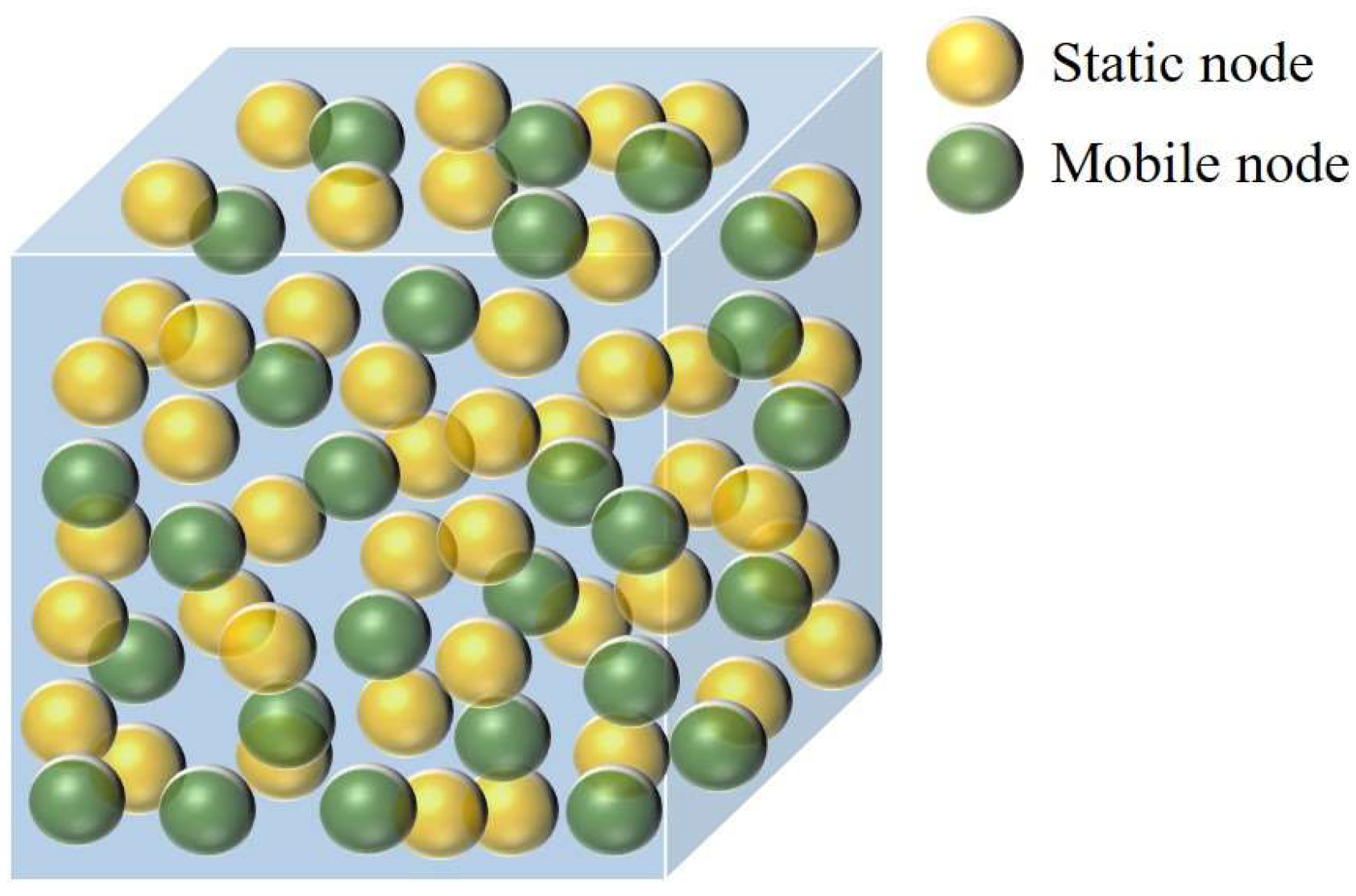
Wireless Sensor Networks (WSNs) are multi-hop self-organizing networks consisting of a set of sensor nodes, small devices, etc., whose task is to monitor events in a specific region and transfer the collected data to a base station (BS) for centralized processing [1,2]. Based on the limitations of real-world scenarios, the deployment of static nodes alone cannot achieve the desired coverage effect, while the deployment of mobile nodes only has the problem of high cost. The hybrid wireless sensor networks composed of static nodes and mobile nodes are more relevant in practical applications such as environmental monitoring, military surveillance, and disaster recovery [3,4]. Through collaborative work between nodes, various environmental monitoring and sensing information can be transmitted to the BS in real-time. If a large quantity of nodes is thrown randomly in reasonable locations, they can cover the target area more precisely [5,6]. However, in real target scenarios, it is often required to throw nodes randomly in a high-density, large-scale manner in sensor networks, but this large-scale random node-throwing approach makes it difficult to deploy nodes in optimal locations at once, resulting in redundant and unperceived regions due to either the over-sparse or dense distribution of nodes in the target region. This node coverage overlap can lead to redundancy in transmitted and received data and channel interference, thus wasting limited energy resources [7].

The nodes rely on their own limited battery power supply, which cannot be replenished in real time, and the secondary replacement of the power supply is not very feasible. As a result, the life cycle of hybrid WSNs is significantly limited. When sensor nodes terminate working because of uneven distribution or exhaustion of energy, malfunction, etc., there are inevitable coverage holes in the network. A coverage blind zone is one which is not perceived by any sensor node in the monitored region. The emergence of blind zones can change the network’s topology, which affects normal communication between nodes and the reliability of data. As sensor nodes may stop working at any time, coverage holes can appear anywhere in the network [8]. In addition, if the coverage holes formed are not repaired, the number and size of coverage holes will gradually increase, disrupt the transmission of data, disconnect from the network, and make certain regions of the network non-monitored [9].

Coverage issues are a fundamental indicator of the quality of service (QoS) of hybrid WSNs [10] that reflect how well the sensor network nodes supervise the monitored area. The detection and repair of coverage holes are becoming increasingly important. With the complexity of the actual environment, the full range of environmental characteristics also needs to be studied [11,12]. In underground infrastructure monitoring, it is often used to monitor storage tanks, power lines, and pipelines. Any faults or leaks can be located and repaired in time by using data shared among sensor nodes [13]. Precision agriculture is a field that is constantly evolving and the need for effective crop production and resource management is improved by monitoring conditions, such as soil mineral composition, moisture, and water content [14]. In medical environment applications, the efficiency and safety of medical devices and the life quality of patients can be effectively improved through patient vital sign monitoring, ward monitoring, medical device monitoring, and drug tracking [15]. In environmental applications, temperature-sensitive sensor nodes in forests are deployed to track the occurrence of fires [16]. Therefore, in this paper, we use the environmental perception importance level indicator as an important factor for consideration when restoring a hole in the node restoration phase.

In this paper, we have devised a distributed detection and multi-objective optimization based on the emperor penguin repair method for coverage holes to solve two key problems in 3D hybrid WSNs, which are hole detection and repair. In addition to receiving and sending data information in hybrid WSNs, static nodes compete for the role of elected group nodes based on their own conditions, and are responsible for aggregating information within their own cells and detecting the source of the hole information that informs the relevant nodes. While mobile nodes are responsible for moving to the optimum location to repair the coverage blind zone based on the received hole information, which uses a multi-objective optimized swarm intelligence algorithm. The contributions are as follows:

• Based on the geometric unit division of the monitoring area, group nodes are selected by using a sum-of-weights method according to static node remaining energy and average distance accumulation values, grouping the management of data information from static and mobile nodes via distributed algorithms, which simplifies network management while ensuring network stability and extending the overall network lifetime.
• A multi-objective fitness function is designed by considering a customized degree of hole region ranking and the uniformity of the remaining energy of the repair nodes, as well as the ratio of the node distance from the hole to the maximum distance travelled. The algorithm prioritizes learning and concentrates on hole regions with high levels of metrics, where the network can meet guaranteed coverage requirements while also performing well in terms of total node energy consumption and node energy uniformity.
• Using network connectivity as a constraint, the optimized emperor penguin algorithm introduces a lens-imaging mapping learning strategy to perturb the location of the repair nodes. It can enhance the algorithm’s ability to search for the hole region in different directions. In this way, the repair nodes can find the optimal repair location to cover and improve the overall efficiency of the network.

The paper is structured as follows: The related works are detailed in Section 2. The network model of a 3D hybrid WSNs and definitions of related terms are presented in Section 3. Section 4 describes the proposed detection and repair algorithm DHD-MEPO in detail. In Section 5, simulation experiments are conducted with the DHD-MEPO and other algorithms to compare and evaluate the network’s performance. Section 6 provides the conclusion and the outlook for further research work in the future.

2. Related Works

In recent years, in the field of sensing coverage, many solutions have been proposed by scholars for the purpose of accurately detecting the position of coverage holes and using effective repair methods to repair holes, thus improving the QoS of WSNs.

Among them, the swarm intelligence optimization algorithm is used for coverage hole detection and repair in a two-dimensional environment. Shyama M et al. [17] presented a multi-objective fault-tolerant routing identification approach combined with a particle swarm algorithm and a genetic algorithm. It integrates coverage, communication cost, proximity, and other factors and uses particle swarm technology to monitor the nodes in the cluster for faults and a genetic algorithm to determine fault-free status. Ali Hallaf et al. [18] divided the specific region based on the static node density deployed in the network, used a round robin working mechanism for the overlap between nodes, and finally added nodes to repair the holes by using a locust optimization algorithm combined with the objective function of the size of the holes and the node movement distance. However, connectivity and the minimum transmission path during the node repair process were not considered. The authors of [19] constructed auxiliary lines to detect underground monitoring area holes by mathematical methods and used tree seeding algorithms with randomness, optimality, and spiral generation techniques to generate new nodes to repair the blind zones; however, the effectiveness of the algorithm complexity was not demonstrated in comparative experiments. Yan et al. [20] proposed consideration of the mobile state of nodes as the motion of artificial fish to repair the holes. Based on a comparison with a correlation threshold, the algorithm introduced jumping and respawning behavior when the population fell into local extremes. It extended the search range of the population, and effectively improved network coverage, which did not demonstrate the performance of the nodes in the aspect of energy consumption as well as connectivity.

Some scholars have proposed a strategy to prioritize the use of boundary nodes to address the coverage hole problem in a two-dimensional scenario. Li et al. [21] focused on the phenomenon of coverage blind zones due to the node failure, the algorithm divided the nodes in the region into the edge and interior nodes, where the nodes are moved by the perceived gravity of the surrounding environment. By calculating the direction and distance of movement, as well as energy consumption, priority is given to moving edge nodes, which effectively reduces unnecessary movement energy consumption. Abhishek Gupta et al. [22] used unsupervised machine learning to identify interior and boundary nodes, and a social spider optimization algorithm was used to adjust Gaussian mixture modelling parameters with maximized expectation to improve the detection rate of coverage holes. The authors of [23] proposed an enhanced hole-boundary detection algorithm for the detection of node failures in networks and connectivity reconstruction after node failures, which effectively avoids network congestion during data transmission and thus improves energy efficiency, but it is difficult to accurately detect the hole boundary when the hole range is large.

Some scholars have also effectively combined mathematical thinking with the coverage hole problem. Lu et al. [24] proposed the development of a prioritization strategy in hybrid heterogeneous networks based on mathematical geometric approaches to determine the size of hole regions and use a limited quantity of mobile nodes to repair the holes, which reduces the redundancy of mobile nodes in the area, with a lack of analysis of the mobile nodes’ energy consumption aspects. The authors of [25] addressed the problem of the high complexity of traditional detection algorithms and proposed a hole detection method on the basis of a simplified Rips complex, in which nodes are classified by combining the degree and clustering coefficients of the complex networks and Turan’s theorem. It determines regular dormant redundant nodes, detects holes from a loop perspective, and achieves high accuracy and low complexity performance of the algorithm, but cannot be directly applied to detecting coverage holes in 3D space in terms of holes. Cansu Cav et al. [26] proposed a new 0–1 mixed integer planning model in smart grid regions, based on optimization, heuristic, and hybrid solutions to find the shortest path for mobile sensor nodes with sufficient energy to cover blind zones in the shortest time while traversing the repair holes. Li et al. [27] balanced the energy consumption of cluster head nodes in the network by establishing a model for the determination conditions of dead node dispersion, selecting cluster head nodes based on the node energy consumption speed parameter, node degree parameter, and distance parameter, as well as affecting the probability of electing cluster heads by determining whether the nodes are in the energy trough or edge zones. Finally, node transmission scheduling and data transmission strategies are introduced to effectively suppress the generation of energy holes. Vipul Narayan et al. [28] proposed an optimization protocol for the coverage overlap and hole problem. A novel method for determining redundant nodes is given in the initialization phase of the network and a sleep–wake method is employed to effectively extend the lifecycle of the network. However, only the hole repair method was proposed, and the hole detection problem was not studied.

Some other scholars have combined the coverage hole problem with fuzzy logic reasoning or routing. Jay Kumar Jain et al. [29] established a Bi-layered WSN-IoT topology. They used a weighting method to elect cluster heads based on factors such as link bandwidth and used an entropy function to perform clustering and merging operations. Fuzzy logic is used to find out which node can recover the hole, and finally the optimal route for data communication is selected according to the emperor penguin algorithm, which effectively solved the problems arising in the field of agriculture. Y. Harold Robinson et al. [30] constructed communication links between sensor nodes through paths and used the level of connectivity as the basis for hole detection. They also used a multi-attribute function constructed by fuzzy rules to compromise on hole events, effectively improving the efficiency of hole detection. Juneja et al. [31] proposed the use of the Red Deer Simulated Annealing model based on the network partitioning of regions to detect holes and moving redundant nodes to repair the holes, which estimates routes based on link stability and then selects relay nodes for data transmission to maximize the network life cycle. The literature [32] proposed a coverage-aware multi-path planning method based on a particle swarm algorithm, which can work in concert with any hole repair algorithm to repair holes caused by faulty nodes and plan efficient paths for mobile collectors.

In the study of covering target points in 3D regions, Dang et al. [33] performed a Voronoi division of nodes in 3D regions, used virtual force algorithms to introduce correlation forces between target points and nodes, and precisely repaired holes according to the priority coverage mechanism of each cell. Hao et al. [34] employed a computational geometry approach to detect 3D surface target region, selected redundant nodes around the hole, determined the repair direction and route, moved the repair nodes to cover the holes based on the effect of virtual forces, and verified the network performance of coverage and connectivity in a realistic scenario.

In the study of 3D underwater complex environments, Zhuang et al. [35] came up with a multi-autonomous vehicle-based coverage hole repair algorithm under multiple constraints in 3D underwater environments, firstly transforming the multiple constraints into an unconstrained multi-objective repair problem Pareto-solving optimum, combining multi-agent tactics and diversity archiving tactics to solve the hole problem, but it is more costly to target different types of sensor node networks. Zhang et al. [36] proposed a clustering-based hole repair algorithm for complex underwater environments. The algorithm used a three-dimensional dense network topology model that treats the coverage hole as a vulnerable region. The temporarily controlled nodes identified the dormant redundant nodes around the vulnerable region and woke up the nodes to repair the vulnerable hole region according to priority. However, the nodes’ performance in the aspect of energy consumption and comparative analysis with other advanced algorithms was not analyzed in the simulation experiments. Amir Chaaf et al. [37] came up with an approach for hole detection and repair of multi-autonomous underwater vehicles based on cluster formation of the ocean depth, dynamic dormancy and wake-up scheduling mechanisms, routing of virtual pictures, and repeater-assisted hierarchical clustering. The introduction of a bi-criteria mayfly optimization algorithm for hole detection effectively reduced the quantity of holes and packet loss rate.

Table 1. Literature review of related works.

Ref.	Year Published	Algorithm Abbreviations	Monitored Area	Network Structure	Methodological Theory	Deficiencies
[17]	2022	FTGSO	Two-dimensional area	Heterogeneous network	Swarm intelligence algorithms	Slow convergence speed and poor accuracy in finding the best
[18]	2022	×		Hybrid network
[19]	2022	MTSA		Homogeneous network
[20]	2020	FSHR		Hybrid network
[21]	2022	×		Homogeneous network	Detection and repair strategies using boundary nodes	Difficult to detect hole boundaries when the hole is large
[22]	2022	SSO-EM GMM		Homogeneous network
[23]	2022	EBHD		Homogeneous network
[24]	2022	VORPH		Hybrid heterogeneous Network	Combining the methods of mathematical theory	High time complexity and long running times
[25]	2020	×		Homogeneous network
[26]	2023	×		Hybrid network
[27]	2022	EHSRA		Homogeneous network
[28]	2022	CHOP		Hybrid network
[29]	2020	×		Heterogeneous network	Fuzzy logic and combination with routing	Poor accuracy in detecting and repairing holes
[30]	2021	FICHD		Homogeneous network
[31]	2022	EMSCOLER		Homogeneous network
[32]	2022	CAMP		Homogeneous network
[33]	2019	3D-VPCA	Three-dimensional space	Homogeneous network	Mathematical geometry methods	Higher energy consumption of the network
[34]	2020	3D-SCHDR	Three-dimensional surface	Hybrid network
[35]	2020	MECHR	Three-dimensional underwater	Heterogeneous network	Clustering and multi-objective optimization methods	The cost of the network is more costly
[36]	2021	×		Heterogeneous network
[37]	2021	ReVOHPR		Heterogeneous network

× indicates that the abbreviation of the algorithm is not given in the literature.

shows the comparison between the algorithms mentioned above.

3. Network Models and Related Definitions

Assume that the network monitoring area is a $k\times k\times k$ 3D target area, discretize the network into $k^3$ target points, the set of target points is $E=\left\{e_1,e_2,\dots ,e_j,\dots ,e_{k^3}\right\}$. $N$ mobile and static nodes are thrown randomly, and the set of nodes is $S=\left\{s_1,s_2,\dots ,s_i,\dots ,s_N\right\}$. All nodes are deployed in the same monitoring region, and the sensing area of each node is a sphere with its own position as the centre of the sphere and a sensing radius of $R_s$. The distribution of hybrid nodes in the target region is shown in Figure 1.

3.1. Perceptual Model

Considering practical application scenarios, the coverage probability of a spherical probabilistic perception model varies with the distance of the nodes. Traditional spherical sensing usually uses a Boolean model, which can lead to errors between the actual coverage and the calculated results. The effect of signal attenuation on the coverage model is considered to avoid the cliff-like perceptual boundaries of traditional Boolean perception models and to match the actual propagation of the node-sensing signal more closely. In this paper, we use a probabilistic perception model that can reflect the properties of the nodes’ perceived distance [38]:

$$P\left(s_i,e_j\right)=\left\{\begin{array}{c}1\\ e^{-\alpha {\lambda }^{\beta }}\\ 0\end{array}\right.\begin{array}{c}d\left(s_i,e_j\right)\le R_s-R_a\\ R_s-R_a<d\left(s_i,e_j\right)<R_s+R_a\\ d\left(s_i,e_j\right)\ge R_s+R_a\end{array},$$

(1)

where $d\left(s_i,e_j\right)$ is the distance between node $s_i$ and target point $e_j$, $d\left(s_i,e_j\right)=\sqrt{{\left(x_i-x_j\right)}^2+{\left(y_i-y_j\right)}^2+{\left(z_i-z_j\right)}^2}$. $R_a$ describes the uncertainty perception capability of the node. $\lambda =d\left(s_i,e_j\right)-R_s-R_a$, $\alpha$ and $\beta$ are the attenuation factors that determine the degree of attenuation. Define $\alpha =\beta =0.5$.

3.2. Energy Model

The energy consumed by nodes in hybrid WSNs includes sending and receiving data, processing data, and other energy consumption [39]. While static nodes consume energy mainly from sending and receiving data, mobile nodes consume a large quantity of energy for movement when repairing coverage holes, in addition to their own energy consumption for sending and receiving data. A node’s energy consumption by sending $l$ bit of data while $d$ meters apart is:

$$E\left(l,d\right)=\left\{\begin{array}{c}l{E}_{elec}+l{\epsilon }_{fs}{d}^2\\ l{E}_{elec}+l{\epsilon }_{amp}{d}^4\end{array}\right.\begin{array}{c}d<d_0\\ d>d_0\end{array},$$

(2)

$$d_0=\sqrt{\frac{{\epsilon }_{fs}}{{\epsilon }_{amp}}},$$

(3)

$E_r\left(l,d\right)$ indicates the node’s energy consumption by receiving $l$ bit of data:

$$E_r\left(l,d\right)=l\times E_{elec},$$

(4)

$E_m$ indicates the node’s energy consumption by moving $d$ metres:

$$E_m=d\times e_0,$$

(5)

where $E_{elec}$ represents the node’s energy consumption by sending and receiving a unit bit of data, $d_0$ is the transmission distance threshold, ${\epsilon }_{fs}$ and ${\epsilon }_{amp}$ are the power amplification circuit loss coefficients under the free-space and multiplex fading models, respectively, and $e_0$ is the node’s energy consumption when it moves a unit distance.

3.3. Definition of Terms

Definition 1.

(Neighbor node): In hybrid WSNs, there exist two nodes $s_i$ and $s_j$ with Euclidean distance $d\left(s_i,s_j\right)<2R_s$, then nodes $s_i$ and $s_j$ are said to be one-hop neighbors of each other.

Definition 2.

(Redundant node): A sensor node $s_i$ is said to be a redundant node of node $s_j$, if its sensing area is overlappingly covered by the sensing area of its neighbor node $s_j$, or if node $s_i$ is jointly covered by the neighbors node $s_{i+1,i=\mathrm{1,2},\dots ,N-1}$ of node $s_j$.

Definition 3.

(Maximum distance travelled by a node): In this paper, the deployed redundant mobile nodes in hybrid WSNs are taken as repair nodes, and a swarm intelligence optimization algorithm is used to determine the optimal repair location of the redundant mobile nodes, so as to repair the coverage holes in the area. The maximum distance that the redundant node $s_i$ can move is limited by considering the node energy consumption and moving distance factors:

$$d_{{max}_i}=\sqrt[n]{\frac{E_{{res}_i}}{l_i}}$$

(6)

where $d_{{max}_i}$ is the maximum distance moved by the redundantly moving node $s_i$; $E_{{res}_i}$ is the current residual energy of node $s_i$; $l_i$ indicates the number of times node $s_i$ has currently moved; the default is 1; and $n$ is usually taken as $2~4$.

Definition 4.

(Mobile node utilization): In hybrid WSNs, nodes are randomly thrown in the monitoring region in a certain ratio. The main job of the mobile node is to take care of the repair of holes, but when the quantity of blind zones in the region is small, some of the mobile nodes will act as static nodes. The ratio of the quantity of mobile nodes to repair holes to the overall quantity of deployed mobile nodes is called mobile node utilization.

4. DHD-MEPO Algorithm

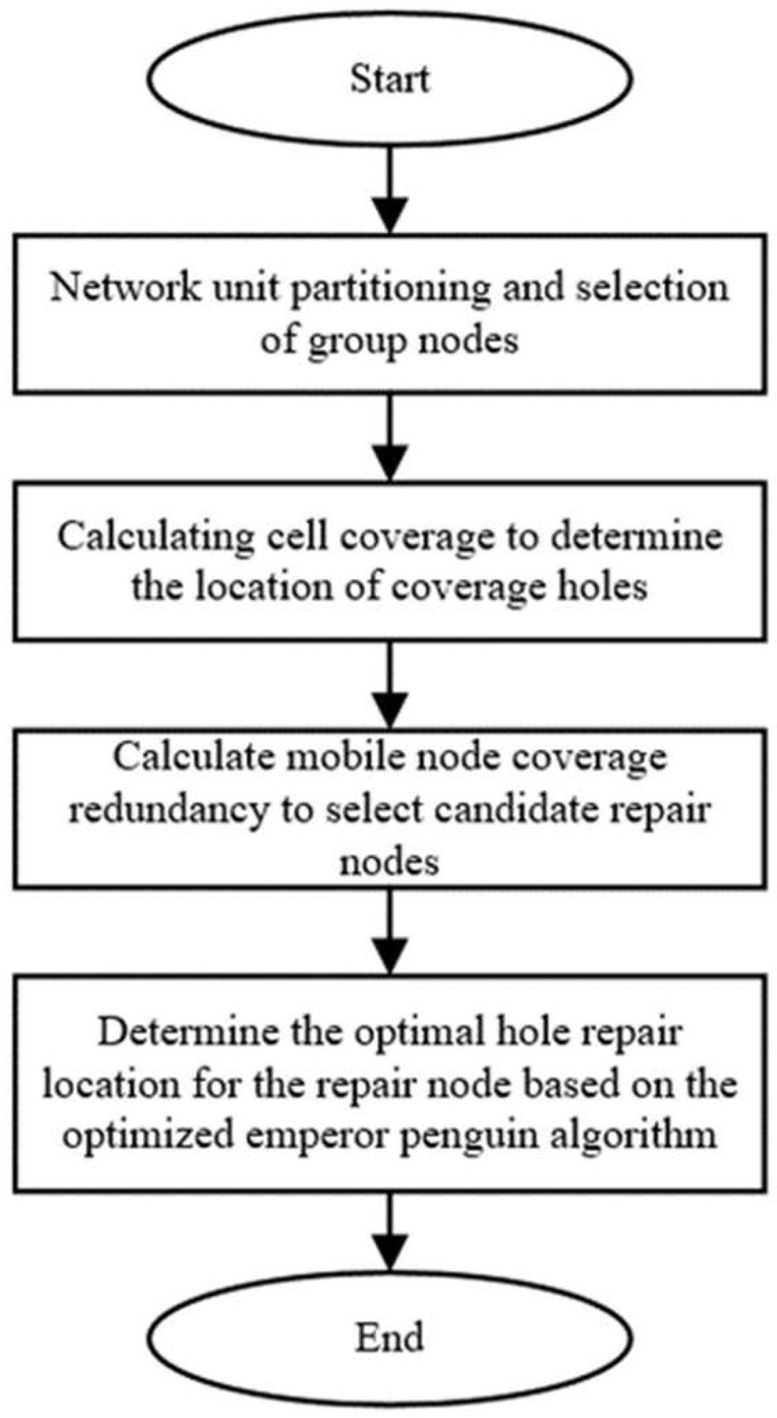
In this section, we come up with a detection and repair approach to address the coverage problem of hybrid WSNs. The approach is organized into two parts. In the coverage hole detection part, for the purpose of facilitating the management of hybrid WSNs, the region is classified as cells on the basis of the quantity of nodes deployed in the region and the nodes’ own sensing range. The group node within each cell is selected according to two parameters: the residual energy value of the static node and the average distance value from the node and the BS, which is responsible for aggregating the data information of the group and then forwarding it to the BS. Then, according to the quantity of target points covered by the nodes in each cell, the coverage ratio of the cell is calculated and the cell ID location covering the hole is determined. In the blind zones’ repair part, the coverage redundancy of mobile nodes in the area is calculated and based on the node redundancy level; then, a suitable mobile node is selected as a candidate repair node responsible for repairing the hole. Finally, a multi-objective fitness function is established, and the final repair location of the repair node is determined using the optimized emperor penguin algorithm to complete the coverage repair and optimization. Figure 2 shows the general flowchart of the DHD-MEPO algorithm.

4.1. Regional Unitization of the Network

There are $N$ mobile sensor nodes and static sensor nodes thrown in the target region, and the quantity of nodes is sufficient. The BS center is responsible for receiving all the data and centralizing the data transmitted by the nodes in turn. That results in an excessive load on the BS, and each node that carries the transmitted data may cause network congestion and consume more energy on the way to its destination. Therefore, to facilitate the management of the network region and save unnecessary energy consumption, the monitoring region is first divided into cells based on the quantity of randomly thrown nodes and the sensing area of the nodes, with each cell representing a unique ID number:

$$V=\frac{4}{3}\pi R_s^3,$$

(7)

$$⌈N_{ideal}⌉=\frac{k^3}{V},$$

(8)

$$D_{ratio}=\frac{⌈N_{ideal}⌉}{N},$$

(9)

$$M=\left\{\begin{array}{c}1,\\ 2^3,\\ 3^3,\\ \dots \end{array}\right.\begin{array}{c}0.9{<D}_{ratio}\le 1\\ 0.8{<D}_{ratio}\le 0.9\\ 0.7{<D}_{ratio}\le 0.8\\ \dots \end{array},$$

(10)

$$c=\frac{k}{\sqrt[3]{M}},$$

(11)

where $V$ is the sensing area of a sensor node; $N_{ideal}$ is the optimal quantity of nodes to be thrown in the region under ideal conditions, rounded upwards. $D_{ratio}$ is the ratio of ideal to actual quantity of nodes thrown, the smaller the ratio, the more nodes the network actually deploys and the greater the number of cells to be divided. $M$ is the total quantity of cells to be divided in the target region, the set is $\mathrm{Q}=\left\{q_1,q_2,\dots ,q_l,\dots ,q_M\right\}$, and $c$ is the edge length of each cell divided.

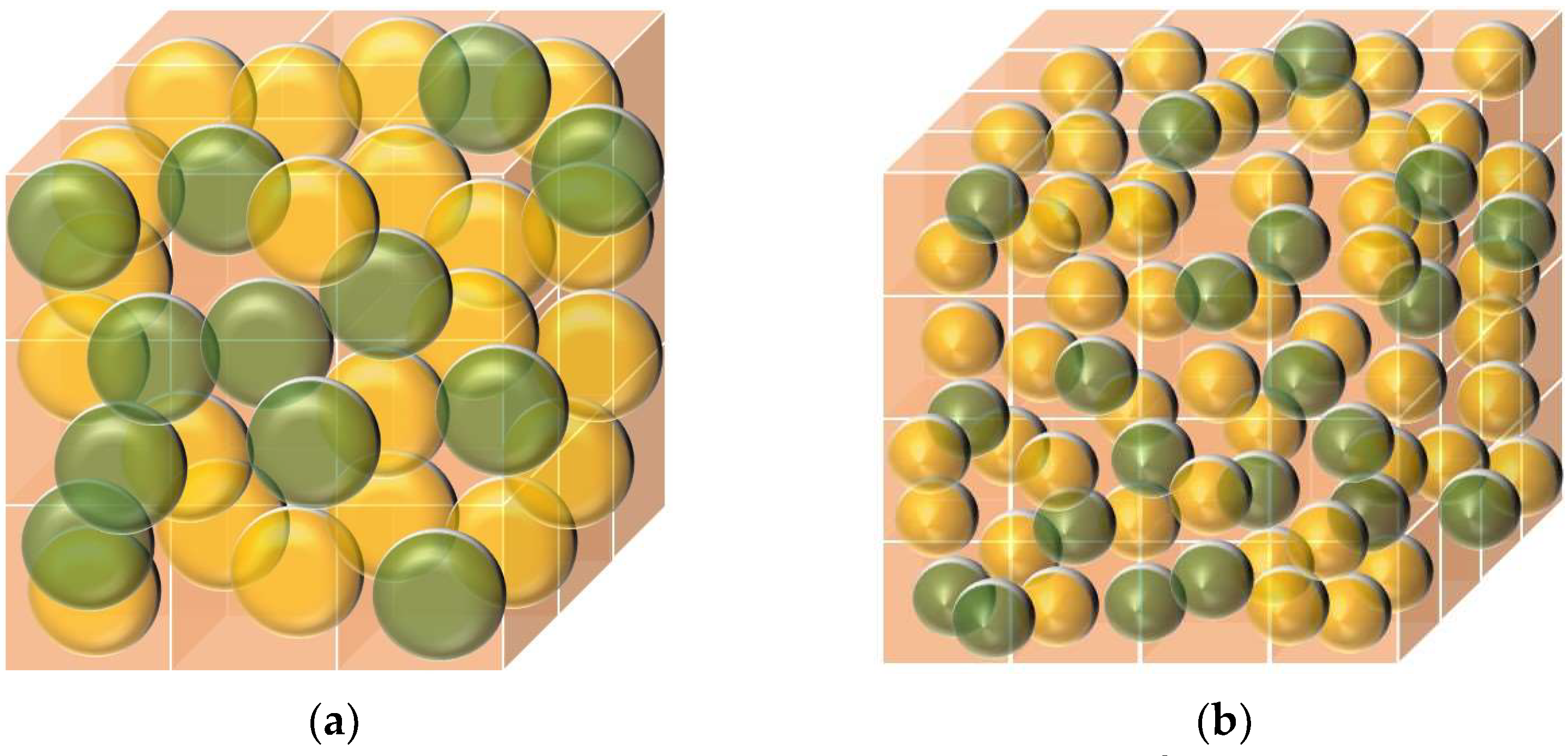
Figure 3 shows a diagram of the target region partitioned into cells according to different node densities.

When the target region is divided into cells based on the density of nodes deployed, a group node is selected in each of the divided cells. The group node is responsible for further data fusion processing of the data received by the group before forwarding it to the BS. That minimizes energy consumption and simplifies network management by processing the information transmitted by the relevant nodes in groups. Load balancing is achieved to lengthen the network lifecycle.

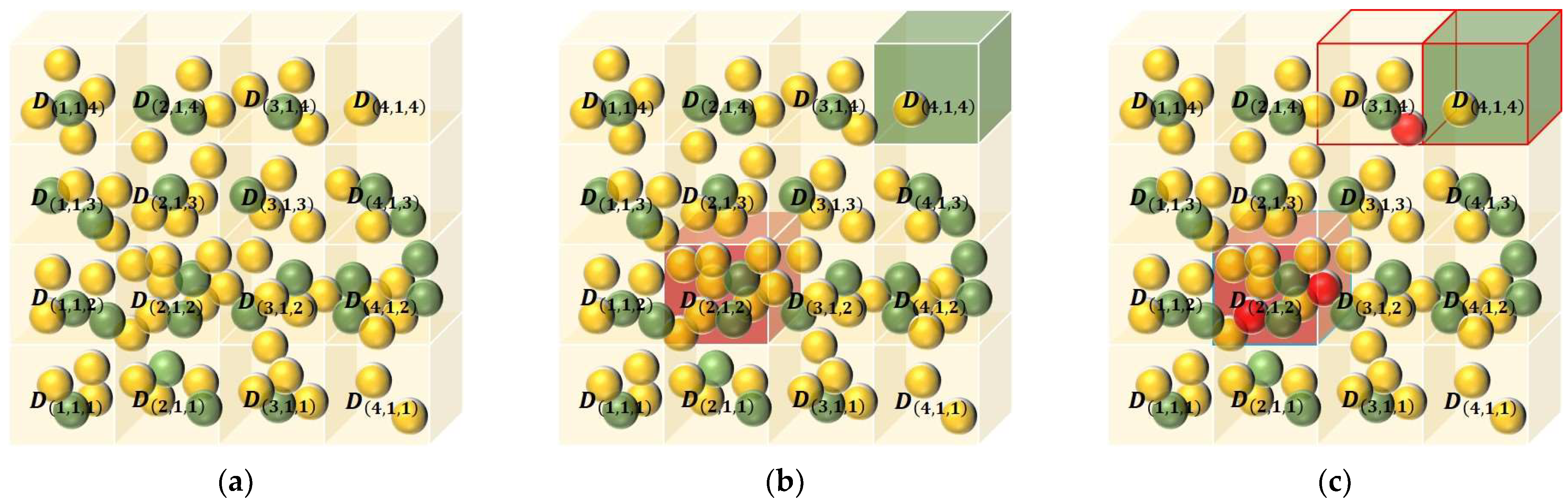
Suppose that the quantity of cell bodies divided is 64 according to Equation (10), as shown in Figure 4a, and any one of its layers is taken for observation. Because of the initial throw of nodes at random, the quantity of nodes within each cell body is uneven. When too many nodes are distributed within a cell body, for example, in Figure 4b, cell body $D_{\left(\mathrm{2,1},2\right)}$ is distributed with 10 nodes. If only one group node is selected within this cell body, it will lead to the group node carrying too much data information volume and quickly exhausting the energy of the group node, so at least two or more group nodes can be set up within this cell to jointly process the data information of the group. When too few nodes are distributed within a cell, e.g., cell $D_{\left(\mathrm{4,1},4\right)}$ has only one node distributed, it would waste the resources of the node if the task of sending and receiving information to the BS is carried out alone. So, merge with neighbor cell bodies that remain connected and select an optimal node as a group node to aggregate data information.

A boundary threshold is set and if the quantity of nodes within the cell is less than the lower limit of minimum threshold, it is merged with the surrounding neighbor cells. If the quantity of nodes within the cell exceeds the upper limit of the maximum threshold, more than two group nodes within the cell will be selected to be responsible for collecting information.

$$Bound=UB-LB,$$

(12)

In this paper, the static nodes within each cell will be selected as group nodes, and the cumulative value of each static node will be aggregated according to two parameters: the residual energy of the static node and the average distance value. The higher the cumulative value, the higher the possibility of the static node being elected as a group node. The role of the group node is also rotated at any time, thus maintaining the stability and overall network lifetime:

$${CV}_{s_i}=Aggregate\left(E_{{res}_i}+\frac{1}{{Adv}_{s_i}}\right),$$

(13)

$${Adv}_{s_i}={\lambda }_{1}d\left(s_i,BS\right)+\frac{{\lambda }_2}{t-1}\sum _{j=1}^{t-1}d\left(s_i,s_j\right),i\ne j,$$

(14)

where $E_{{res}_i}$ is the residual energy of static node $s_i$; ${Adv}_{s_i}$ is the weighted sum of the average distance value between static node $s_i$ and other nodes within its own cell and the distance value to the BS; and ${\lambda }_1$, ${\lambda }_2$ are usually taken as 1/2. $t$ is the quantity of nodes distributed within the cell.

The three red nodes in Figure 4c are the group nodes of the cell $D_{\left(2,1,2\right)}$ and the cell $D_{\left(3,1,4\right)}$, $D_{\left(4,1,4\right)}$, respectively.

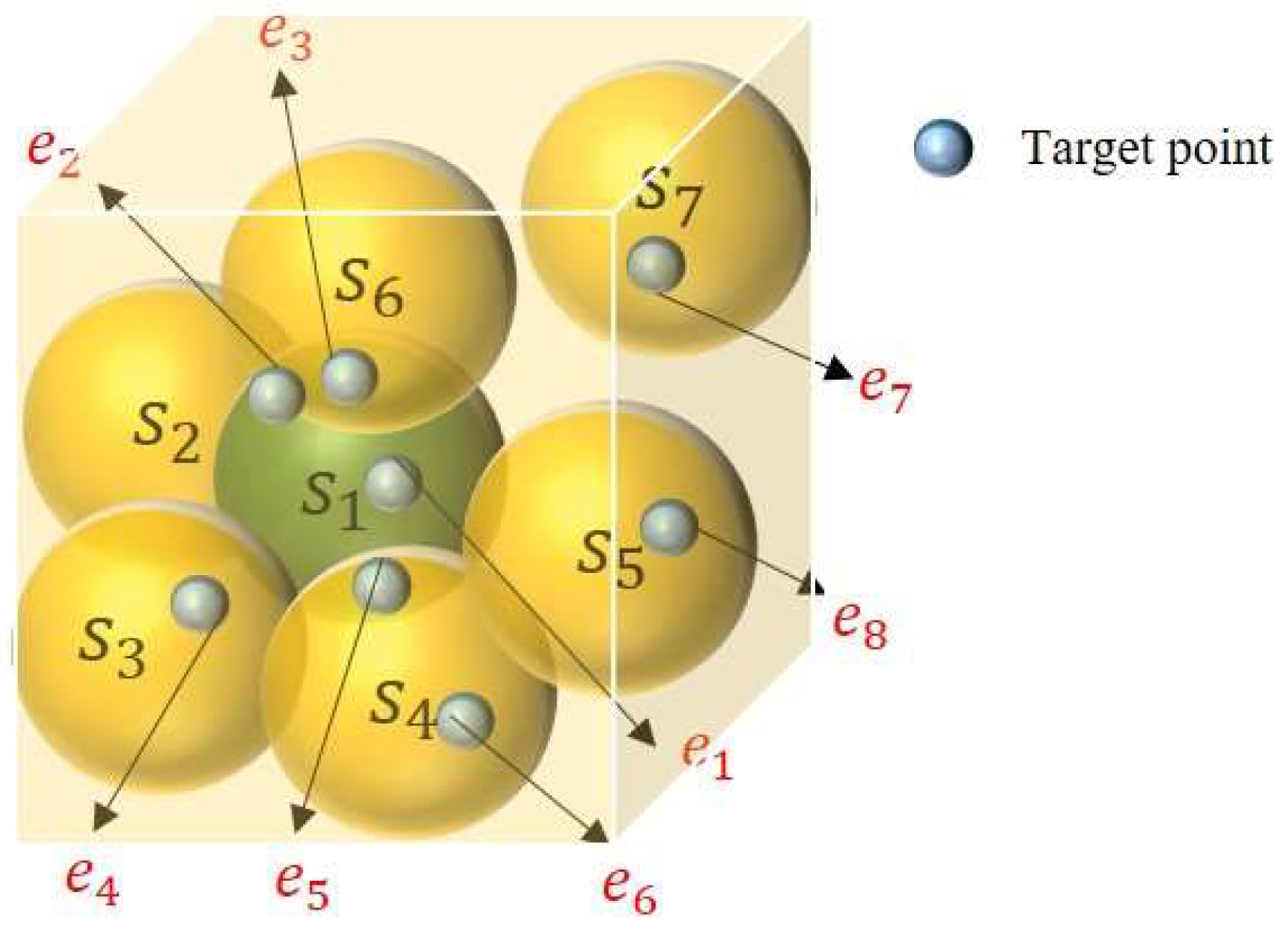
4.2. Calculation of cell Coverage

Based on the divided cell side length $c$, it is determined that there are $c^3$ target points within each cell, and the coverage ratio of each cell is calculated to determine whether there are coverage holes within each cell, and thus the position of the coverage blind zones. A sensor node can cover multiple target points, while the same target point is also covered by multiple sensor nodes, as illustrated in Figure 5. Target point $e_2$ is covered by sensor nodes $s_1$, $s_2$, and $s_6$ at the same time, indicating that there are three sensor nodes covering target point $e_2$ at the same time, then the coverage of sensor node $s_1$ on target point $e_2$ at this time is 1/3, and so on. Then, any one sensor node $s_i$ within the cell has a coverage of all target points $e_j,j=1,2,\dots ,c^3$ within the cell, the sum of coverage can be calculated as:

$$P\left(s_i,c^3\right)=\sum _{j=1}^{c^3}P\left(s_i,e_j\right),$$

(15)

The coverage of all nodes within the cell for all target points within the cell in aggregate, i.e., cell coverage, is:

$$P_{D_{\left(x,y,z\right)}}=\frac{\sum _{i=1}^{t}P\left(s_i,c^3\right)}{c^3},$$

(16)

where $t$ is the quantity of sensor nodes distributed within the cell $D_{\left(x,y,z\right)}$.

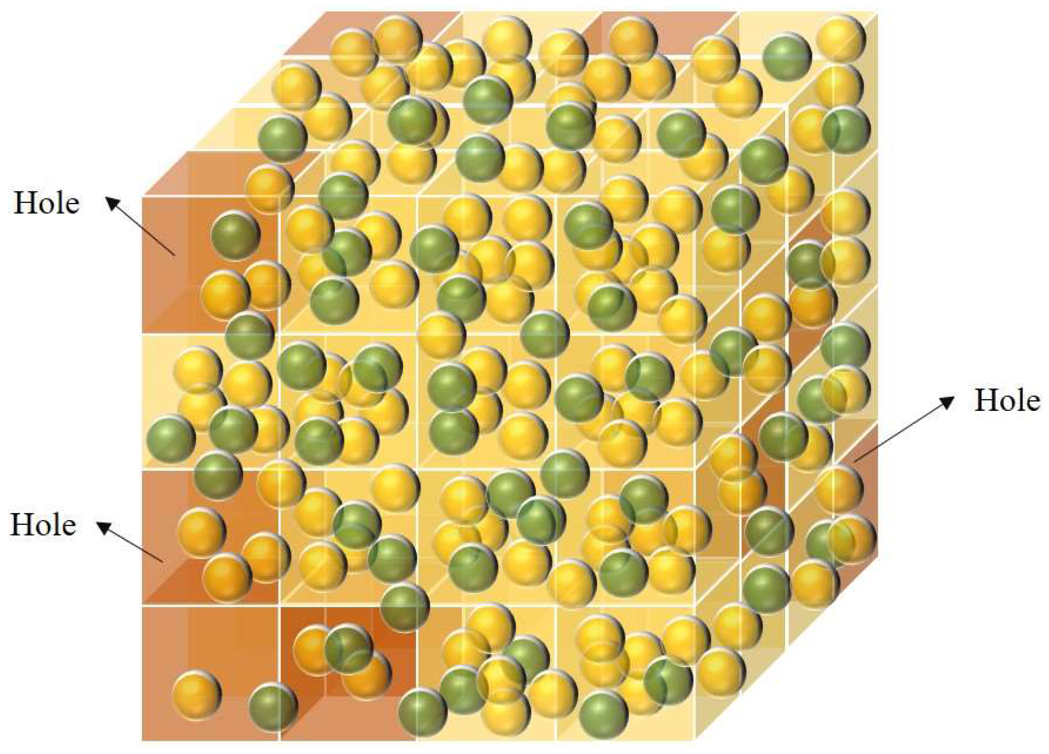
If the coverage of a cell is greater than 90%, it means that there is no coverage hole in the cell; otherwise, there is a coverage hole in the cell. As shown in Figure 6, the cell marked in red indicates that there is a hole in the cell and the redundant nodes in the target region need to be moved to cover the hole.

Algorithm 1 is the algorithm covering the hole detection phase:

Algorithm 1. Detection phase algorithm.

1: Initialization: edge length $k$ of the network, number of network cells $M$, cell ID number $D_{\left(x,y,z\right)}$, cell edge length $c$, number of nodes $N$, node perception range $V$

2: $⌈N_{ideal}⌉=\frac{k^3}{V}$, $D_{ratio}=\frac{⌈N_{ideal}⌉}{N}$//Calculation of the node ratio based on the quantity of nodes and the node sensing range

3: The quantity of cells is divided according to $D_{ratio}$, with each cell ID being $D_{\left(x,y,z\right)}$

4: ${CV}_{s_i}=Aggregate\left(E_{{res}_i}+\frac{1}{{Adv}_{s_i}}\right)$//Cumulative values according to static node remaining energy and average distance values

5: Select the group nodes for each cell $D_{\left(x,y,z\right)}$

6: for (i = 1; $i\le N$; i++) do

7: $P\left(s_i,c^3\right)=\sum _{j=1}^{c^3}P\left(s_i,e_j\right)$//Calculate the sum of each node’s coverage of all target points within the cell

8: $P_{D_{\left(x,y,z\right)}}=\frac{\sum _{i=1}^{t}P\left(s_i,c^3\right)}{c^3}$//Calculate the coverage of each cell

9: if Cell coverage >90% then

10:  No holes within the unit

11: else

12:  The unit has a hole in it

13: end if

14: end for

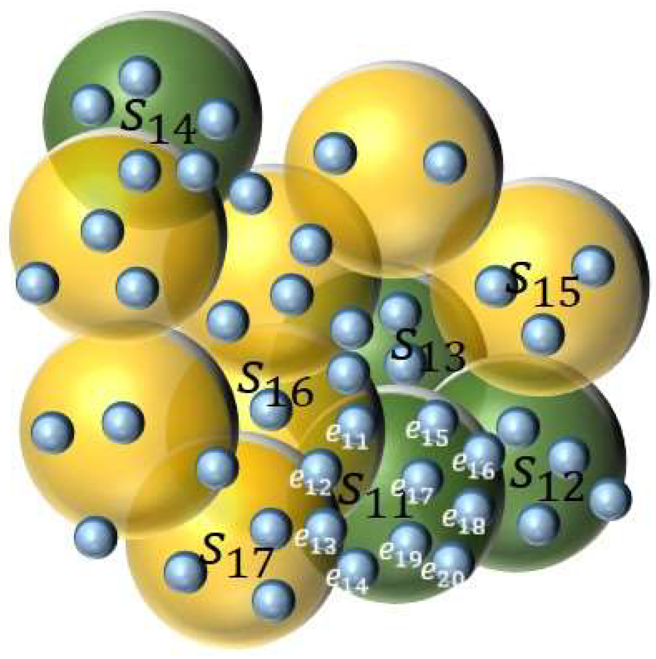
4.3. Calculating Mobile Node Coverage Redundancy

When repairing holes, to ensure cell coverage on the basis of meeting the actual application requirements, we need to select redundant mobile nodes in the target region to repair, using the resources of redundant mobile nodes to find hole coverage as effectively as possible and successfully improving the efficiency of the nodes. Therefore, candidate repair nodes need to be identified. When selecting candidate repair nodes, we first select from within the cell with the highest cell coverage. Assuming that certain mobile sensor nodes are densely distributed within a cell with a cell coverage of 90% or more, according to the calculated redundancy of the target points within the mobile node coverage cell, we judge that the redundancy is higher than 90% as a candidate repair node. Taking mobile node $s_{11}$ in Figure 7 as an example, the quantity of target points within the coverage cell of $s_{11}$ is 10. The statistics of these 10 target points being covered by other neighbor nodes around $s_{11}$ are shown in

Table 2. Coverage of $s_{11}$ by surrounding neighbor nodes.

	${\mathit{s}}_{11}$ Covering Target Points	${\mathit{e}}_{11}$	${\mathit{e}}_{12}$	${\mathit{e}}_{13}$	${\mathit{e}}_{14}$	${\mathit{e}}_{15}$	${\mathit{e}}_{16}$	${\mathit{e}}_{17}$	${\mathit{e}}_{18}$	${\mathit{e}}_{19}$	${\mathit{e}}_{20}$
${\mathit{s}}_{11}$ Neighbor Nodes
$s_{12}$		0	0	0	0	1	1	1	1	0	1
$s_{13}$		1	0	0	0	1	0	1	0	0	0
$s_{16}$		1	1	0	0	0	0	0	0	0	0
$s_{17}$		0	1	1	1	0	0	0	0	0	0
${Cover}_{nei}$		1	1	1	1	1	1	1	1	0	1

, where 1 means covered by neighbor nodes and 0 means not covered.

The set of candidate repair nodes $R_m$ is determined by calculating the redundancy of each mobile node within the cell. The redundancy of mobile node $s_i$ covering the target point is calculated as follows:

$${Red}_{s_i}=\frac{\sum _{j=1}^h{Cover}_{nei}}{h}\ast 100$$

(17)

where $h$ is the total quantity of target points covered by mobile node $s_i$; ${Cover}_{nei}$ indicates whether target point $e_j$ is covered by neighboring nodes of node $s_i$. If it is covered by neighbor nodes, ${Cover}_{nei}$ is 1, otherwise it is 0. The greater the cumulative value of ${Cover}_{nei}$, the greater the chance of the mobile node becoming a repair node.

4.4. Optimizing the Emperor Penguin Algorithm to Repair Holes

Once the set of candidate repair nodes $R_m$ is determined, we propose to use the optimized emperor penguin algorithm to determine the best location for repair nodes to repair the hole. The emperor penguin algorithm (EPO) [40] is a novel swarm intelligence algorithm presented by Dhiman G and Kumar V in 2018, where emperor penguins behave as a cluster to warm each other against the wind and cold when severe weather comes. It is characterized by few parameters and high convergence accuracy.

4.4.1. Initialization

A penguin population consisting of a set of candidate repair nodes $R_m$ is created, and the location data of the candidate repair nodes are a set of solution spaces. Initially, the location information of static nodes and other mobile nodes that have currently identified a good location is input. During the monitoring of the area, the repair nodes need network connectivity to exchange data information related to the collaborative task of forwarding the information collected in the hole region to neighbor nodes. So, connectivity is maintained by being adjacent to at least one other node that has already established a good location. That is equivalent to the algorithm’s feature of emperor penguins gathering in a block for shelter and warmth in harsh winter conditions.

Hybrid WSNs use network connectivity as a constraint during the repair of holes to guarantee that the nodes transmit the data information collected in the hole region to the BS in a single or multi-hop way during the repair of the hole:

$$AM\left(s_i,s_j\right)=\left\{\begin{array}{c}1,\\ 0,\end{array}\right.\begin{array}{c}0<d\left(s_i,s_j\right)\le 2R_s\\ d\left(s_i,s_j\right)>{2R}_s\end{array}$$

(18)

where $AM\left(s_i,s_j\right)$ is either 0 or 1, with 1 indicating connectivity between nodes $s_i$ and $s_j$, and no connectivity otherwise. According to the judgment method of Equation (18), the adjacency matrix $AM$ corresponding to the nodes in the target region is constructed, so that the connectivity of the network can be judged by using $AM$, and then the connectivity matrix $C$ is:

$$C=AM+{AM}^2+{AM}^3+\dots +{AM}^{N-1}$$

(19)

When all the elements in the matrix are 1, the network is connected. If the elements in the matrix are not all 1, it indicates that the network is not connected.

4.4.2. Multi-Objective Fitness Function Design

A multi-objective fitness function is designed by combining the important occupancy of the hole region, the energy balance coefficient of the candidate repair node, and the distance of the repair node from the blind zones. The three sub-goal factors collectively characterize the amount of coverage that a repair node can achieve by moving.

1. 

Significant percentage of hole regions

Based on environmental learning to sense the importance level of the target monitoring region, the environmental monitoring region is learned iteratively, and the importance level of each cell area is continuously changed based on the data information value of the target point and the surrounding environment’s customization factors. By setting the importance value of each cell area, the repair nodes will prioritize covering the hole regions with a high importance value, and the repair nodes can cooperate with each other to prioritize learning and concentrate on the hole regions with a high cell importance value index, which can save the nodes unnecessary energy consumption and collecting data information of unimportant blind zones. Therefore, the importance value of the cell hole region is an important factor to be considered when coverage blind zones occur.

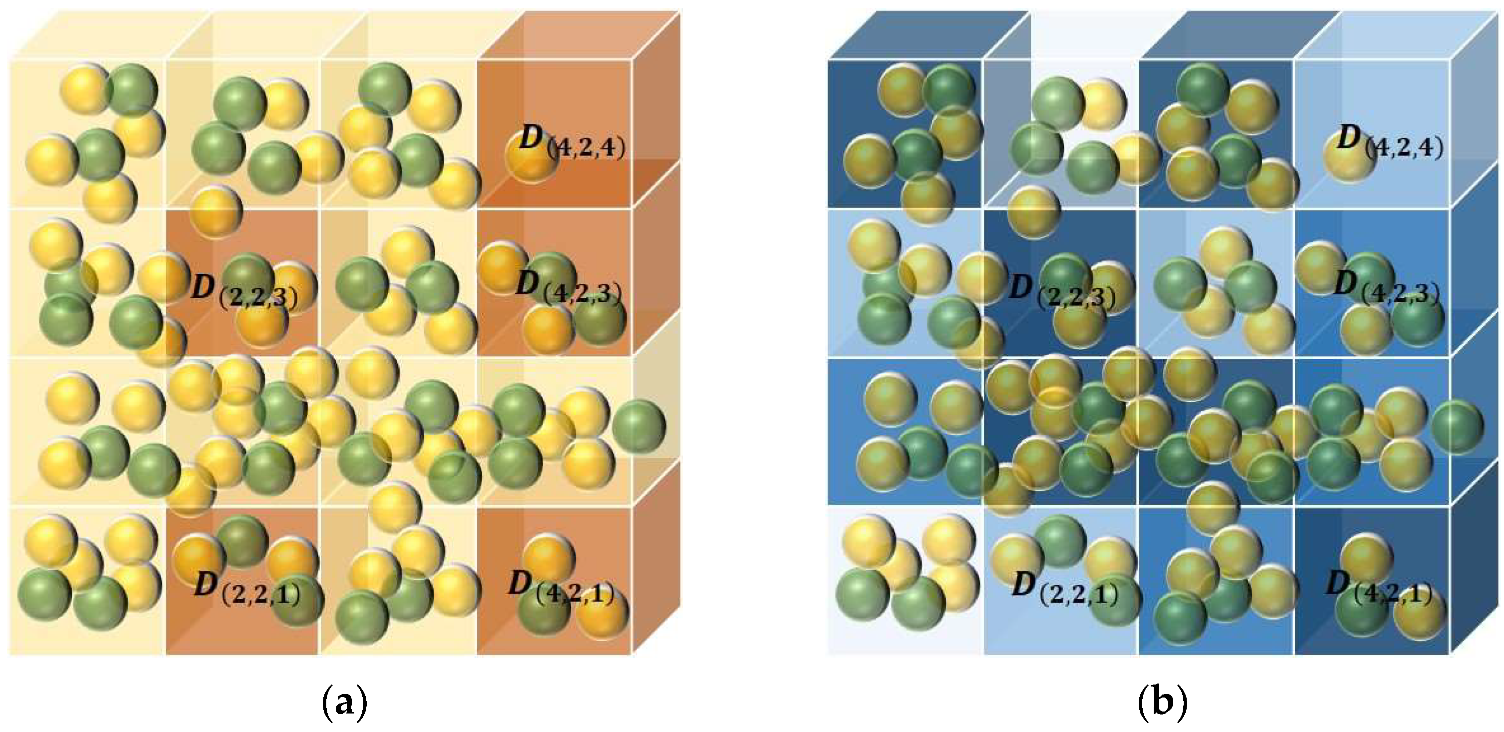
Based on the custom environmental information perception factors, the quantity of important levels is determined based on the quantity of cells divided into each layer of the area. For example, as shown in Figure 8a for a part of the target region, the red area is the hole region, as each layer is divided into four cells. As shown in Figure 8b, the area cells will be divided into four levels, the importance level $G_{\left(x,y,z\right)}$ from one to four increasing, in the figure with the color from increasing from light to dark importance level in turn. The quantity of each important area rank and the location of the same rank distribution are uneven, reflecting the dynamic and random nature of environmental perception areas. From Figure 8, it can be seen that cell hole $D_{\left(4,2,1\right)}$ and cell hole $D_{\left(2,2,3\right)}$ have rank 4, so they are the hole regions that the repair nodes prioritize for coverage.

2. 

Energy balance factor of candidate repair nodes

The energy balance coefficient $\theta$ for a candidate repair node is calculated as:

$$\theta =\frac{Max\left(E_{{res}_p}\right)-Min\left(E_{{res}_p}\right)}{\frac{1}{m}\sum _{p=1}^m{E}_{{res}_p}}$$

(20)

where $E_{{res}_p}$ is the residual energy of candidate repair node $s_p$; $m$ is the quantity of candidate repair nodes; and $\theta$ denotes the energy consumption equalization factor of the repair nodes. The larger the value of $\theta$, the more nodes unbalanced the energy consumption, and conversely, the more balanced the energy consumption.

3. 

Distance of the repair node from the blind zone

The ratio between the distance of the repair node from the blind zone and the maximum distance the repair node can move is judged, and only the case when the ratio is less than 1 is considered. The smaller the ratio, the closer the node is to the hole. If the ratio is not less than 1, the repair node is directly excluded from repairing this hole repair. The maximum distance, $d_{{max}_p},$ that the repair node can move is calculated by Equation (6).

The multi-objective fitness function can be expressed as:

$$Fitness={\omega }_1\left(\frac{1}{k/c}\times G_{\left(x,y,z\right)}\right)+{\omega }_2\left(1-\theta \right)+{\omega }_3\left(1-\frac{d\left(s_p,D_{hole\left(x,y,z\right)}\right)}{d_{{max}_p}}\right)$$

(21)

where $G_{\left(x,y,z\right)}$ denotes the importance rank ratio occupied by this coverage hole region and $d\left(s_p,D_{hole\left(x,y,z\right)}\right)$ denotes the distance of this repair node from this coverage hole. ${\omega }_1$, ${\omega }_2,$ and ${\omega }_3$ are weighting coefficients, ${\omega }_1+{\omega }_2+{\omega }_3=1$. The determination of the weighting parameters is given in Section 5.1.

The location of each moving emperor penguin is determined by the value of the objective function in Equation (21) to determine whether or not to repair at that hole location, with higher fitness values indicating greater coverage gain for the repair node.

4.4.3. Lens Imaging Mapping Learning Strategy to Determine Optimal Location of Repair Nodes

The formula for updating the original location of emperor penguins is as follows:

$$X_{ep}^{t+1}=X_{best}^t-\Gamma L_{ep}$$

(22)

where $X_{ep}^{t+1}$ is the position of the emperor penguin updated at $t+1$ iterations; $X_{best}^t$ is the optimal solution position of the emperor penguin individual after $t$ iterations; $\Gamma$ is the influence vector factor of the emperor penguin volume to avoid conflicts between emperor penguin individuals; and $L_{ep}$ is the distance of the emperor penguin from the center.

The original location update formula for emperor penguins has no other variation operations, making the population less diverse and difficult to search in all directions in a multi-dimensional space. In particular, the emperor penguin optimal individual position $X_{best}^t$ guides the emperor penguin population’s hugging behavior throughout the search process, i.e., during the global phase and the local phase, and determines the extent to which the overall EPO search performance is superior. In the original algorithm, the update of the optimal emperor penguin position relies on the judgment of the fitness value after each iteration; this may lead to the algorithm becoming trapped in a local optimum and it being difficult to jump out of it, thus weakening the overall search ability of the algorithm.

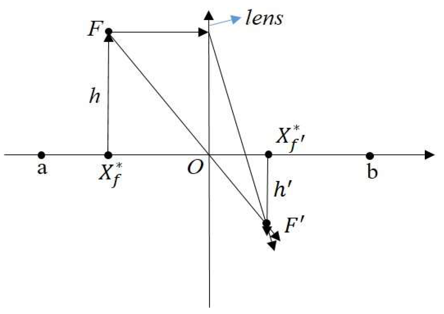
Therefore, the capacity of the algorithm to search in different directions is enhanced by introducing a lens-imaging mapping learning strategy to perturb the positions of emperor penguin individuals caught in local extremes and improve the ability of the optimal emperor penguin individuals to lead the population. The principle of lenticular imaging is shown in Figure 9.

The mathematical mapping formula is:

$$\frac{\left(a+b\right)/2-X_f^{*}}{X_{f^{\prime }}^{*}-\left(a+b\right)/2}=\frac{h}{h^{\prime }}=\mu$$

(23)

where $\mu$ is the scaling factor, collating Equation (23) gives the position of $X_{f^{\prime }}^{*}$ as:

$$X_{f^{\prime }}^{*}=\frac{a+b}{2}+\frac{a+b}{2\mu }-\frac{X_f^{*}}{\mu }$$

(24)

where $X_f^{*}$ in the emperor penguin algorithm then denotes the original optimal individual position of the emperor penguin; and $X_{f^{\prime }}^{*}$ denotes the new optimal position of the emperor penguin individuals generated by lens mapping; the lens imaging strategy can be used to generate new individuals and increase the variety of the population by dynamically adjusting the parameter $\mu$ according to Equation (26):

$$X_{best}\left(new\right)=\frac{ub+lb}{2}+\frac{ub+lb}{2\mu }-\frac{X_{best}}{\mu }$$

(25)

$$\mu =\frac{1}{2}+e^{\frac{10t-5T}{T}}$$

(26)

where $ub$ and $lb$ are the upper and lower bounds of the target area; and $T$ is the maximum quantity of iterations. As can be seen from Equation (26), the scaling factor $\mu$ changes with the number of iterations, showing a state of smaller values in the early part of the process and larger values in the later part of the process, balancing the ability of the algorithm to require a global search in the early part of the process and a local search in the later part of the process of the emperor penguin individuals.

Therefore, the optimized position is updated as follows:

$$X_{ep}^{t+1}\left(new\right)=X_{best}^t\left(new\right)-\Gamma L_{ep}$$

(27)

Algorithm 2 is the algorithm covering the hole repair phase:

Algorithm 2. Repair phase algorithm.

Input: initial position of the set of candidate repair nodes $R_m$

Output: optimal location for repair nodes

1: Initialization: quantity of target points $h$ covered by each mobile node, quantity of mobile nodes in the network $N_m$

2: for (i = 1; $i\le N_m$; i++) do

3: ${Red}_{s_i}=\frac{\sum _{j=1}^h{Cover}_{nei}}{h}\ast 100$//Calculate the coverage redundancy of each mobile node

4: if Coverage redundancy < 90% then

5:  The mobile node is not elected as a candidate for repair

6: else

7:  The mobile node is selected as a candidate for repair

8: end if

9: end for

10: Determine the set of candidate repair nodes $R_m$

11: for (r = 1; $r\le m$; r++) do

12:  $X_{best}\left(new\right)=\frac{ub+lb}{2}+\frac{ub+lb}{2\mu }-\frac{X_{best}}{\mu }; \mu =\frac{1}{2}+e^{\frac{10t-5T}{T}}; X_{ep}^{t+1}\left(new\right)=X_{best}^t\left(new\right)-\Gamma L_{ep}$//Calculate the location of the repair node

13: if the fitness function is higher than the previous then

14:  The current position is the best position to repair the node

15: else

16:  Return 13, recalculate node position

17: end

18: end for

19: return optimal location for repair nodes

4.5. Time Complexity Analysis

For an algorithm, the time complexity measures how fast the algorithm runs and thus reflects the efficiency of the algorithm. $N$ is the population size, $T$ is the maximum quantity of iterations, $M$ is the quantity of area cell bodies, $c$ is the edge length of the cell bodies, $m$ is the quantity of repair nodes, $N_m$ is the quantity of mobile nodes and $d$ is the spatial dimension. The time complexity of unitizing the network region is $O\left(1\right)$, the time complexity of calculating the cell coverage is $O\left(N\times c^3+M\right)$, the time complexity of calculating the mobile node coverage redundancy is $O\left(N_m\right)$, and finally, optimising the emperor penguin algorithm to repair the holes, the time complexity of the initialization calculation is $O\left(m\times d\right)$ and the time complexity of the multi-objective fitness function is $O\left(3\times m\right)$. The time complexity of introducing the lens-imaging mapping learning strategy is $O\left(m\right)$, and the time complexity required for the whole algorithm is $O\left(\mathrm{T}\times \left(1+\left(N\times c^3+M\right)+N_m+\left(m\times d\right)+\left(3\times m\right)+m\right)\right)=O\left(\left(N\times c^3+M+N_m+(d+4)\times m\right)\times T\right)$.

5. Simulation Experiments

This paper uses the MATLAB 2019a platform to perform simulation experiments on the feasibility of the detection and repair algorithms in this paper. DHD-MEPO with 3D-Voronoi partitioning for WSNs (3D-VPCA) proposed in [33], a novel confident information coverage hole-healing algorithm (C-CICHH) proposed in [41], the random algorithm (RA), an enhanced mobile sink-based coverage optimization and link-stability estimation-based routing protocol (EMSCOLER) proposed in [31], and an improved energy-efficient routing protocol (IERP) proposed in [42] were compared. The validation is carried out in the small-scale region $10\times 10\times 10 {\mathrm{m}}^3$ and the large-scale region $100\times 100\times 100 {\mathrm{m}}^3$, respectively. A total of 35 static nodes and 15 mobile nodes are randomly thrown for a target region of $10\times 10\times 10 {\mathrm{m}}^3$, and 70 static nodes and 30 mobile nodes for a target region of $100\times 100\times 100 {\mathrm{m}}^3$. The parameters set in the simulation experiments are presented in

Table 3. List of simulation parameters.

Parameters List	Parameter Values
Scope of the monitoring region	$10\times 10\times 10 {\mathrm{m}}^3$/$100\times 100\times 100 {\mathrm{m}}^3$
Quantity of iterations	200
Quantity of nodes deployed	50/100
Quantity of static nodes	35/70
Quantity of mobile nodes	15/30
Node perception radius	$2 \mathrm{m}$/$15 \mathrm{m}$
Initial energy per node	4 J/33 J
Circuit loss factor in free space	$10 \mathrm{p}\mathrm{J}/\left(\mathrm{b}\mathrm{i}\mathrm{t}/{\mathrm{m}}^2\right)$
Circuit loss factor under multiplex fading	$0.0013 \mathrm{p}\mathrm{J}/\left(\mathrm{b}\mathrm{i}\mathrm{t}/{\mathrm{m}}^4\right)$
Energy consumed to move a unit distance	$0.004 \mathrm{J}/0.033 \mathrm{J}$

.

5.1. Determination of Weighting Parameters

By reading the relevant literature, we set three different sets of weighting parameters, namely ${\omega }_1=0.3 ,{\omega }_2=0.4 ,{\omega }_3=0.3$, ${\omega }_1=0.2 ,{\omega }_2=0.5 ,{\omega }_3=0.3$ and ${\omega }_1=0.35 ,{\omega }_2=0.3 ,{\omega }_3=0.35$. By observing the changes in network coverage brought about by different weighting parameters at different numbers of iterations, the analysis of Figure 10 shows that the network coverage with weighting parameters of ${\omega }_1=0.3 ,{\omega }_2=0.4 ,{\omega }_3=0.3$ is higher than that of other two groups, so we determine that the parameters of the multi-objective fitness function are ${\omega }_1=0.3 ,{\omega }_2=0.4 ,{\omega }_3=0.3$, which can effectively improve the network performance.

5.2. Coverage Analysis

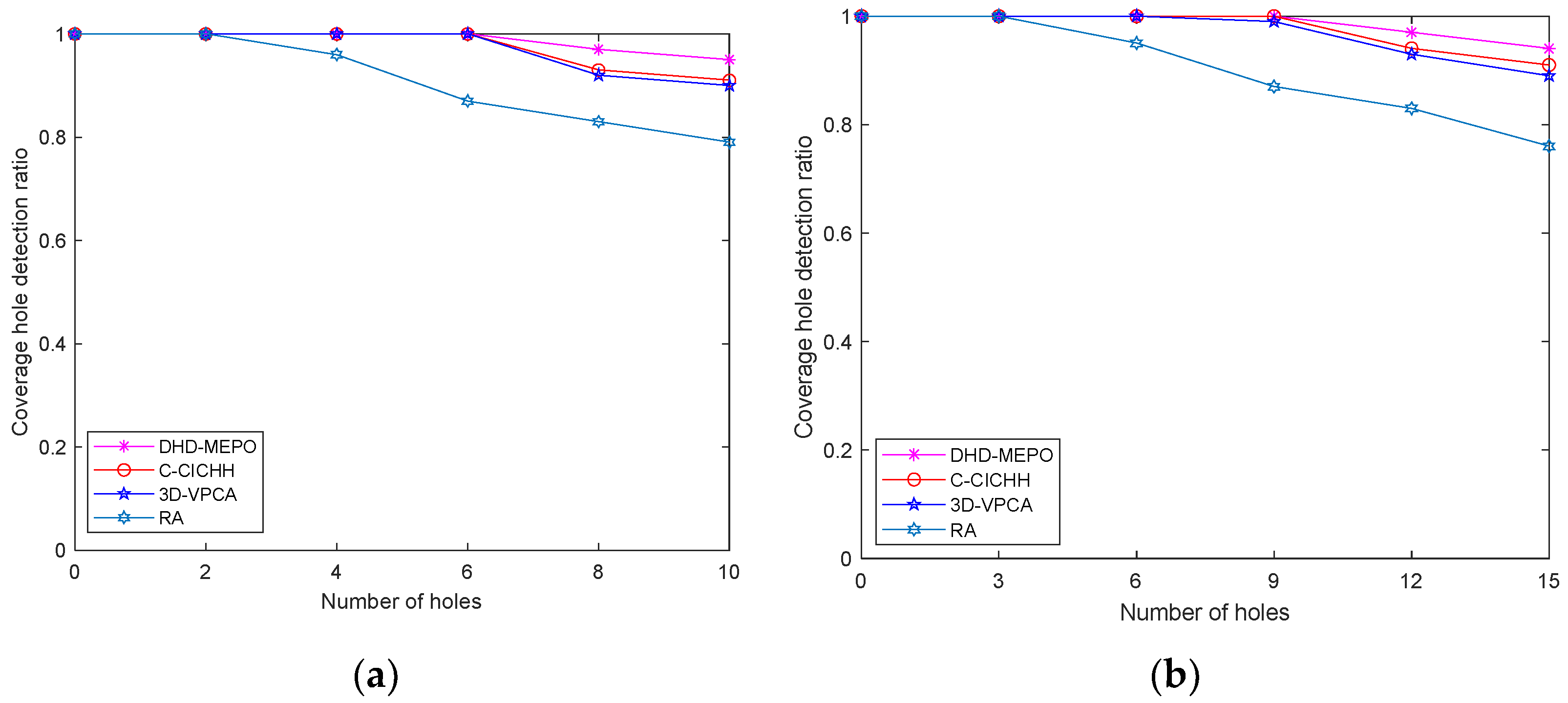
By setting the quantity of nodes in different regions to 50 and 100, respectively, Figure 11 displays the relationship between the quantity of holes and the coverage hole detection rate for the four algorithms in the target regions of $10\times 10\times 10 {\mathrm{m}}^3$ and $100\times 100\times 100 {\mathrm{m}}^3$. The analysis of Figure 11a,b shows that the hole detection rate of the different algorithms varies with the quantity of holes in the region. From Figure 11a, the hole detection ratio of the DHD-MEPO, C-CICHH, and 3D-VPCA algorithms are all 1 when the quantity of holes is up to 6. After the quantity of holes exceeds 6, the detection rates of the algorithms for the holes all decrease, but the DHD-MEPO algorithm decreases slowly compared to the other algorithms. At the quantity of holes of 12, it still has a detection rate of above 0.95 for holes. Similarly, in Figure 11b, the algorithm is in a dominant position for the detection of holes even in a network of $100\times 100\times 100 {\mathrm{m}}^3$. The detection rates of the C-CICHH and 3D-VPCA algorithms are consistently close to each other for holes, while the RA algorithm performs the worst.

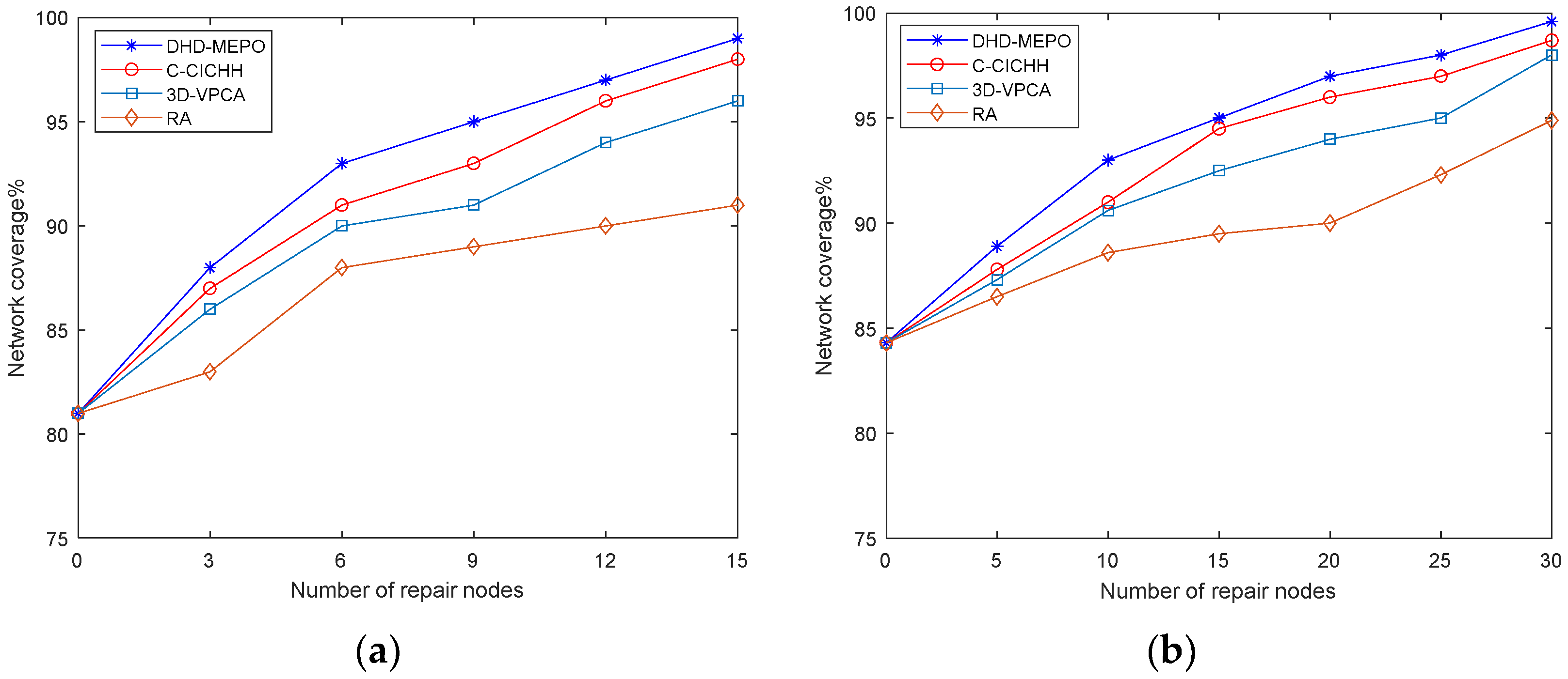
The quantity of covered holes was set to 8 and 12 in different regions. Figure 12 displays the connection between the total quantity of repair nodes and the coverage rate of the four algorithms in the target regions of $10\times 10\times 10 {\mathrm{m}}^3$ and $100\times 100\times 100 {\mathrm{m}}^3$. The analysis of Figure 12a shows that in the $10\times 10\times 10 {\mathrm{m}}^3$ region, as the quantity of repair nodes increases, the location of the blind zones in the region is gradually covered. Using the algorithms in this paper to repair, the coverage rate grows faster than using the other three algorithms and is always in the leading position, and the coverage rate of DHD-MEPO and C-CICHH reaches 95% when the quantity of repair nodes is 12 above. The coverage rates of C-CICHH and 3D-VPCA are close to each other in the interval of 5–10 repair nodes, and the coverage rate of DHD-MEPO is close to 1 in the interval of 30 repair nodes. The reason for DHD-MEPO’s leading coverage rate at different quantity of repair nodes is that the lens-imaging mapping learning strategy in the optimized emperor penguin algorithm is used to perturb the current optimal position of the repair node in the repair phase, which enhances the search capability of the algorithm in different directions and enables the node to find the appropriate optimal position to cover the hole faster.

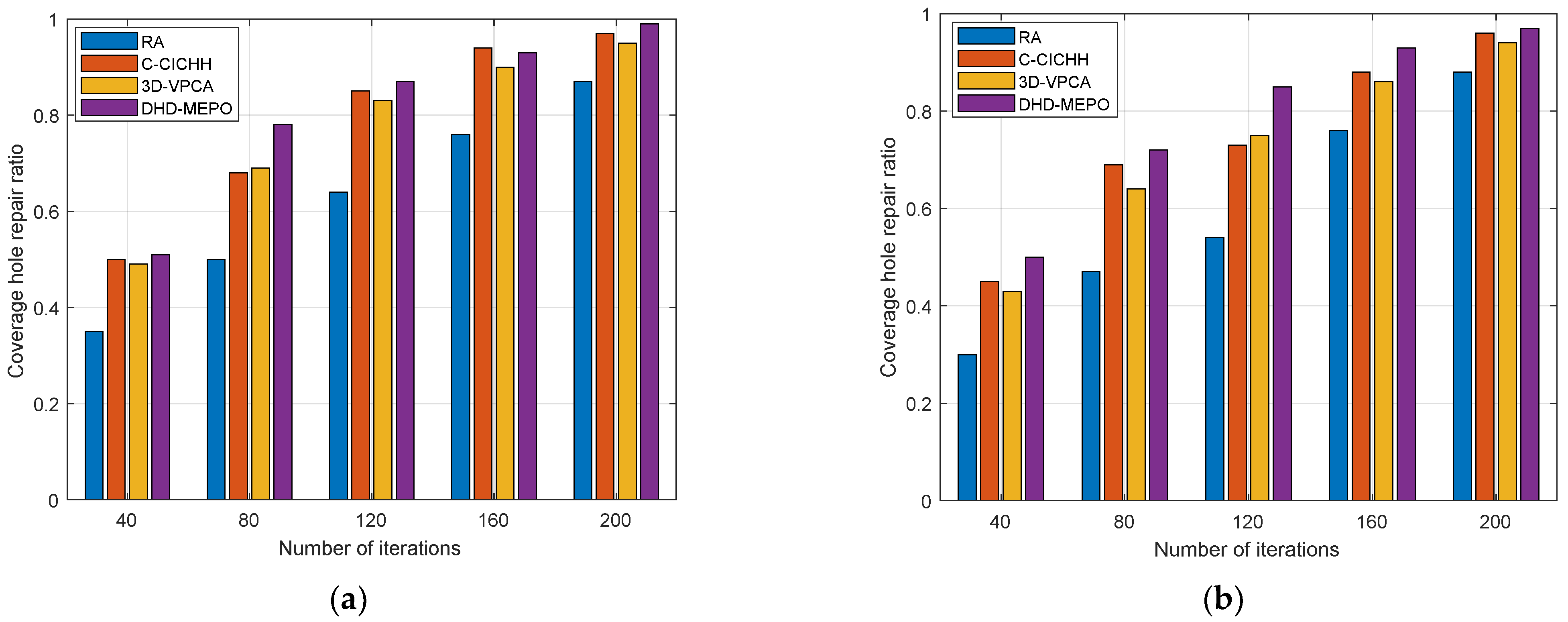
The number of repair nodes is set to 12 and 18 in different regions. Figure 13 shows the relationship between the quantity of iterations and the hole repair ratio for the four algorithms in the target regions of $10\times 10\times 10 {\mathrm{m}}^3$ and $100\times 100\times 100 {\mathrm{m}}^3$. As the quantity of iterations of the algorithm run increases, some of the nodes in the region stop working due to energy depletion, so the quantity of holes as well as their location is constantly changing. The analysis of Figure 13 shows that after 200 rounds of work with all four algorithms, the hole repair rate essentially reaches over 90%. In Figure 13a, at 160 rounds of algorithm work, it can be observed that the C-CICHH hole repair ratio is higher than that of DHD-MEPO. The reason for this analysis may be that the multi-objective fitness function is followed in the process of repairing holes using the algorithms in this paper. In the fitness function, this paper takes the important percentage of the covered hole area as an optimization objective, therefore, the repair of the hole. Even though the current size of the hole region is small, it has a high regional importance rating, so priority is given to repair the hole region. The other algorithms choose to prioritize repairing a large hole region within the acceptable movement range of the mobile node so as to achieve the actual need for repairing the hole. In Figure 13b, at 120 rounds of work, 3D-VPCA has a slightly higher repair ratio than C-CICHH, mainly because the 3D-VPCA algorithm sets the uncovered target point as the source of attraction for the repair node during the repair process, using virtual forces to increase this gravitational influence between the node and the target point and forcing the accelerated node to move to cover the blind zone.

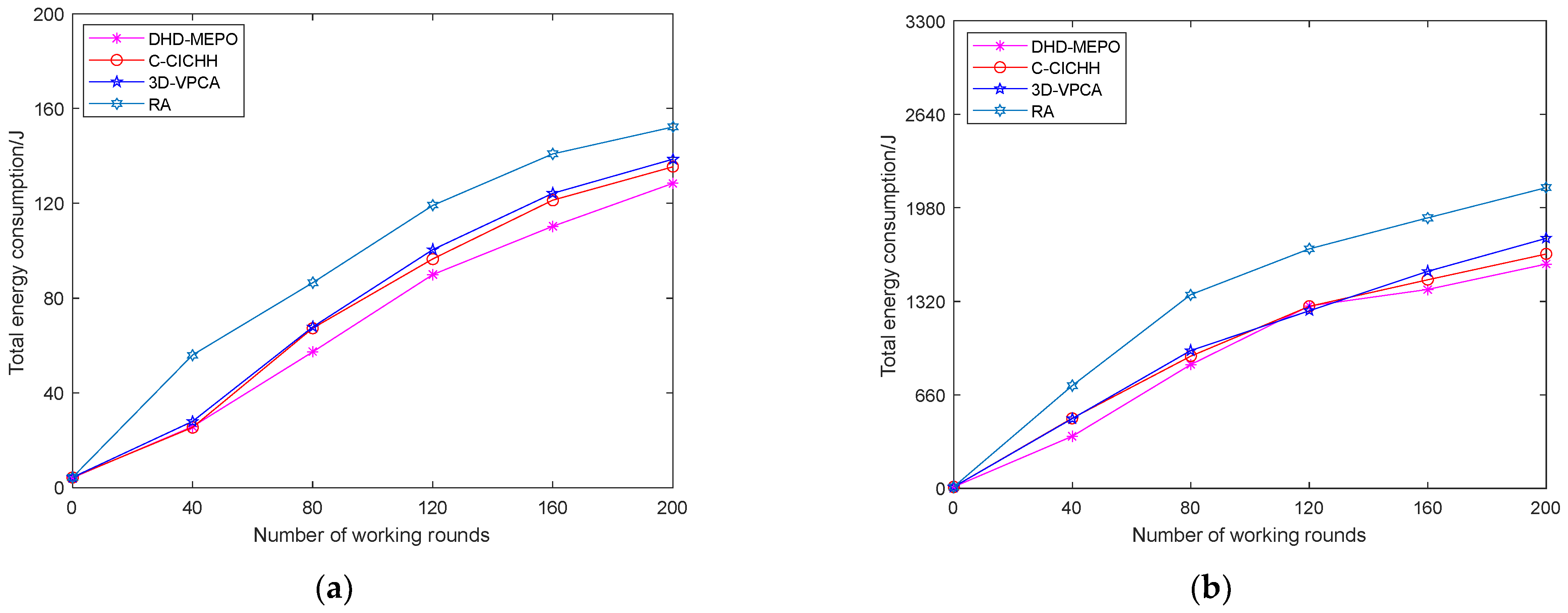
5.3. Energy Consumption Analysis

Each of the four algorithms is subjected to several independent experiments under the same conditions to obtain the graph in Figure 14 between the quantity of working rounds and the total energy consumed in a target area of $10\times 10\times 10 {\mathrm{m}}^3$ and $100\times 100\times 100 {\mathrm{m}}^3$. The analysis of Figure 14a shows that the nodes’ overall energy consumption using the RA algorithm is more than that consumed by the other three algorithms, and the nodes’ overall energy consumption reaches 152.3 J after 200 rounds of operation. The nodes’ overall energy consumption using the DHD-MEPO and C-CICHH and 3D-VPCA methods is approximately equal before the algorithm has been run 40 times. Because the main source of the sensor nodes’ energy consumption in the current network is receiving and sending data information, and the repair nodes have not all started to work yet, the energy consumed by moving the distance to repair the hole is not obvious. The analysis of Figure 14a,b shows that after 200 rounds of work using the DHD-MEPO algorithm, the total node consumption is 128.4 J and 1584 J, respectively, which is a significant saving of energy for the nodes compared to the energy consumed using other algorithms, improving the energy efficiency and extending the lifecycle of hybrid WSNs. The reason for this is that by dividing the network into cells and selecting groups of nodes to manage other nodes within the cell and aggregate data information during the hole detection process, the coordination avoids the unnecessary energy consumed by all nodes to send information to the center of the BS. The analysis of the 120 rounds of algorithm work in Figure 14b displays that DHD-MEPO is slightly higher than C-CICHH and 3D-VPCA, mainly because in the process of repairing holes, DHD-MEPO will give priority to the hole regions with a high importance level, even though there are hole regions near the current repair node that are a shorter distance to repair. However, the level degree of these hole regions is not high, so it will move a longer distance to repair the region with a higher importance level within the longest distance to which this node can move according to the multi-objective fitness value, so the energy consumed will be high.

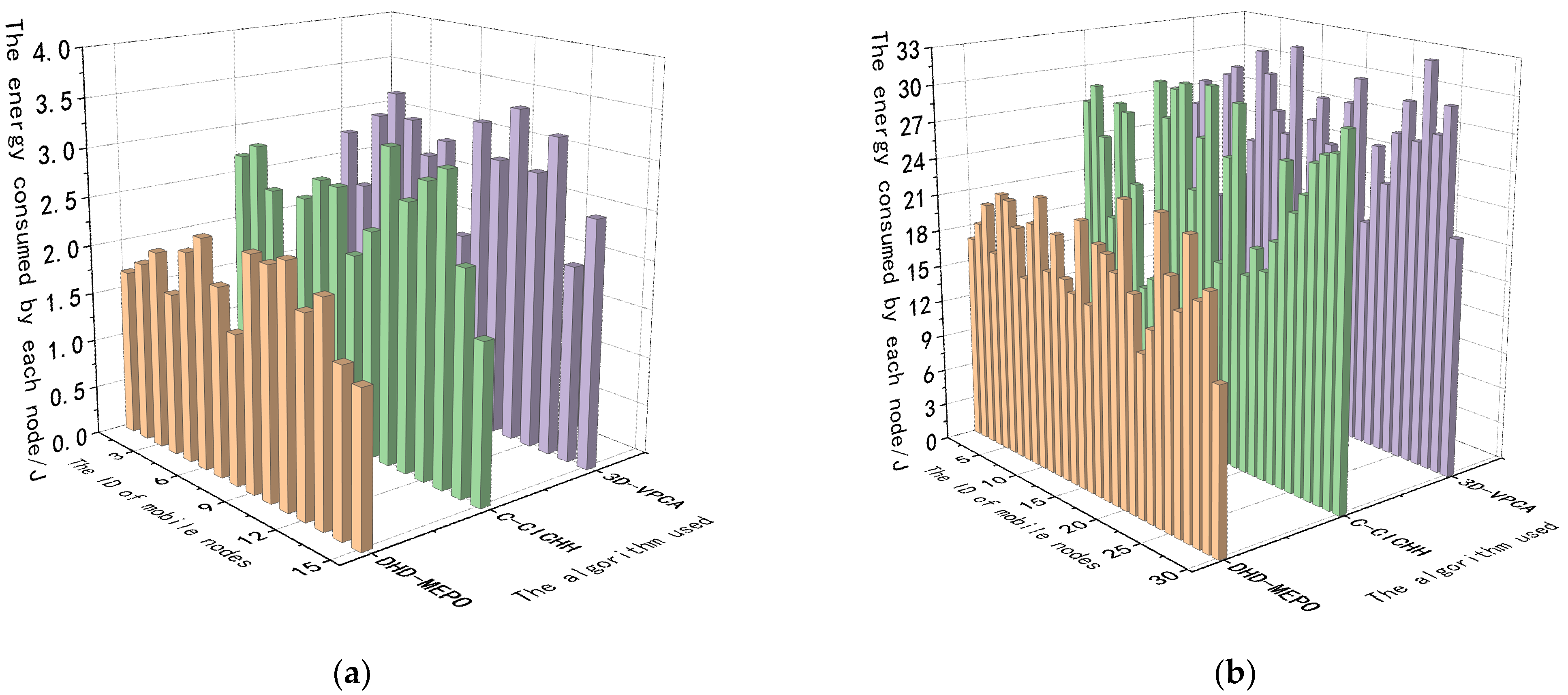
The relationship between the DHD-MEPO and C-CICHH, 3D-VPCA algorithms in terms of each mobile node ID and energy consumed in a target region of $10\times 10\times 10 {\mathrm{m}}^3$ and $100\times 100\times 100 {\mathrm{m}}^3$ is analyzed. From Figure 15a,b, it can be seen that 3D-VPCA performs the worst, C-CICHH slightly outperforms 3D-VPCA, and DHD-MEPO significantly outperforms 3D-VPCA and C-CICHH when considering the overall energy consumption and the uniformity of the mobile node energy consumption. Compared with C-CICHH and 3D-VPCA, a single node’s maximum energy consumption and the nodes’ uniformity of the overall energy consumption are effectively reduced by the inclusion of the energy balance coefficient of the repair nodes as a measure in the multi-objective function setting process, so that all repair nodes will maintain a certain level of energy balance to repair the holes. In contrast, 3D-VPCA and C-CICHH minimize the nodes’ overall energy consumption to some extent, but do not allow for the optimization of the uniformity of energy consumption of the mobile nodes, which leads to the performance differences shown in Figure 15.

5.4. Mobile Node Utilization Analysis

Analyze the connection between mobile node utilization and the quantity of mobile nodes in a target region of $10\times 10\times 10 {\mathrm{m}}^3$ and $100\times 100\times 100 {\mathrm{m}}^3$ for the DHD-MEPO. By setting the proportion of mobile nodes to 20%, 40%, and 60% of the total quantity of nodes in hybrid WSNs in different monitoring regions, the mobile node utilization of the DHD-MEPO is observed for a different quantity of working rounds. The analysis of Figure 16 shows that at the beginning when the algorithm works for 40 rounds, the utilization rate of mobile nodes is not high, especially when mobile nodes account for 60% of the total quantity of nodes. Even after 200 rounds of the algorithm, the proportion of mobile nodes effectively repairing holes is less than 50%, so if a large amount of mobile nodes is thrown in hybrid WSNs, not only are the resources of mobile nodes not effectively used, i.e., most nodes will act as static nodes responsible for receiving and sending messages, but there will also be an increase in the network’s cost. After the comparative analysis of the mobile node ratio in Figure 16, we chose to deploy 15 mobile nodes initially in the experimental area of $10\times 10\times 10 {\mathrm{m}}^3$ and 30 mobile nodes initially in the area of $100\times 100\times 100 {\mathrm{m}}^3$, which can ensure that the mobile nodes are used effectively as fully as possible and can improve the energy efficiency of the nodes.

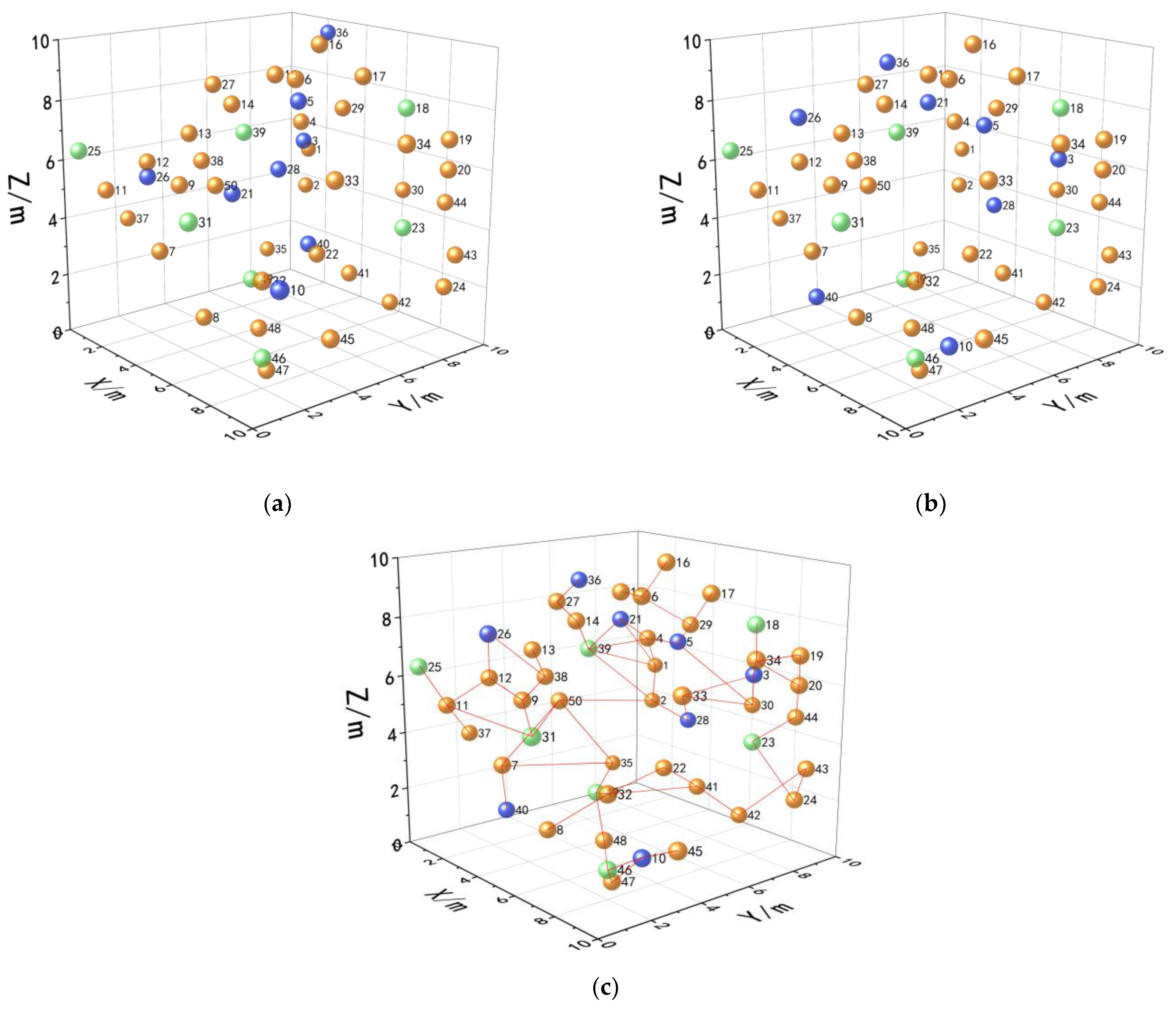
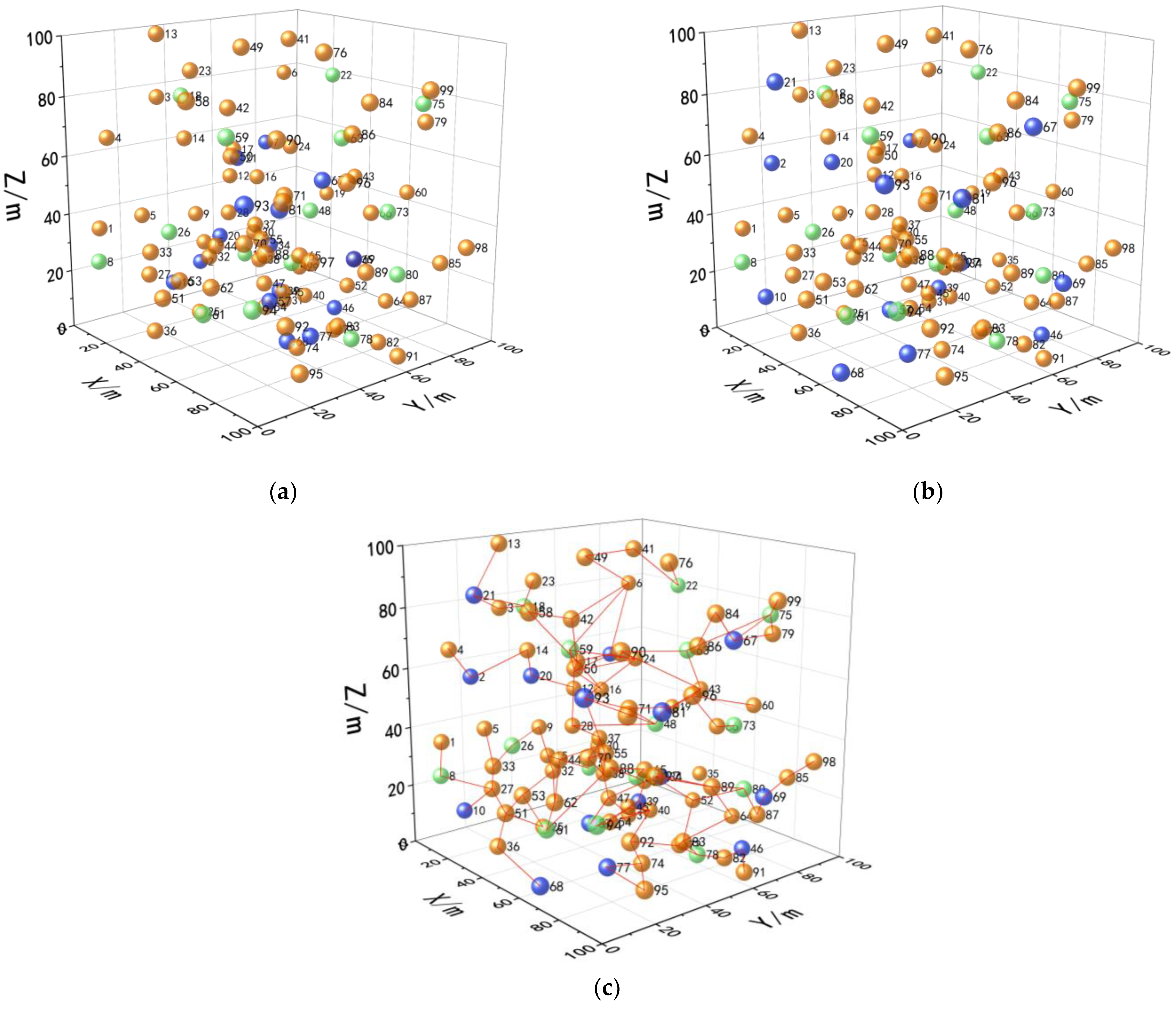
5.5. Connectivity Analysis

After using the detection and repair method of the DHD-MEPO, the connection between the connectivity of the sensor nodes is analyzed. The orange ball in the figure is the static node, the green ball is the mobile node, and the blue ball is the node for repairing the hole. The candidate repair nodes for the target region of $10\times 10\times 10 {\mathrm{m}}^3$ and $100\times 100\times 100 {\mathrm{m}}^3$ are selected by the DHD-MEPO, and the initial location maps are shown in Figure 17a and Figure 18a. The repair nodes use the emperor penguin optimized repair algorithm, which uses the lens-imaging mapping learning principle to perturb the position of the repair node to enhance the ability to search for the hole region in different directions. The position after repairing the hole is shown in Figure 17b and Figure 18b, the optimal position of the repair node is found according to the multi-objective function as well as the constraints and Figure 17c and Figure 18c verify the network connectivity after the repair node completes the task of repairing the hole. According to Equation (18), $AM\left(s_i,s_j\right)=1$ represents the network connection between two nodes and the Kruskal method is used to construct the minimal spanning tree. The algorithm is proven to satisfy the condition that the nodes in the network repair the hole to meet the coverage requirement while also ensuring network connectivity, so that the repair node can instantly send the data information sensed in the hole area to the neighbor nodes and eventually hand over to the BS center for processing.

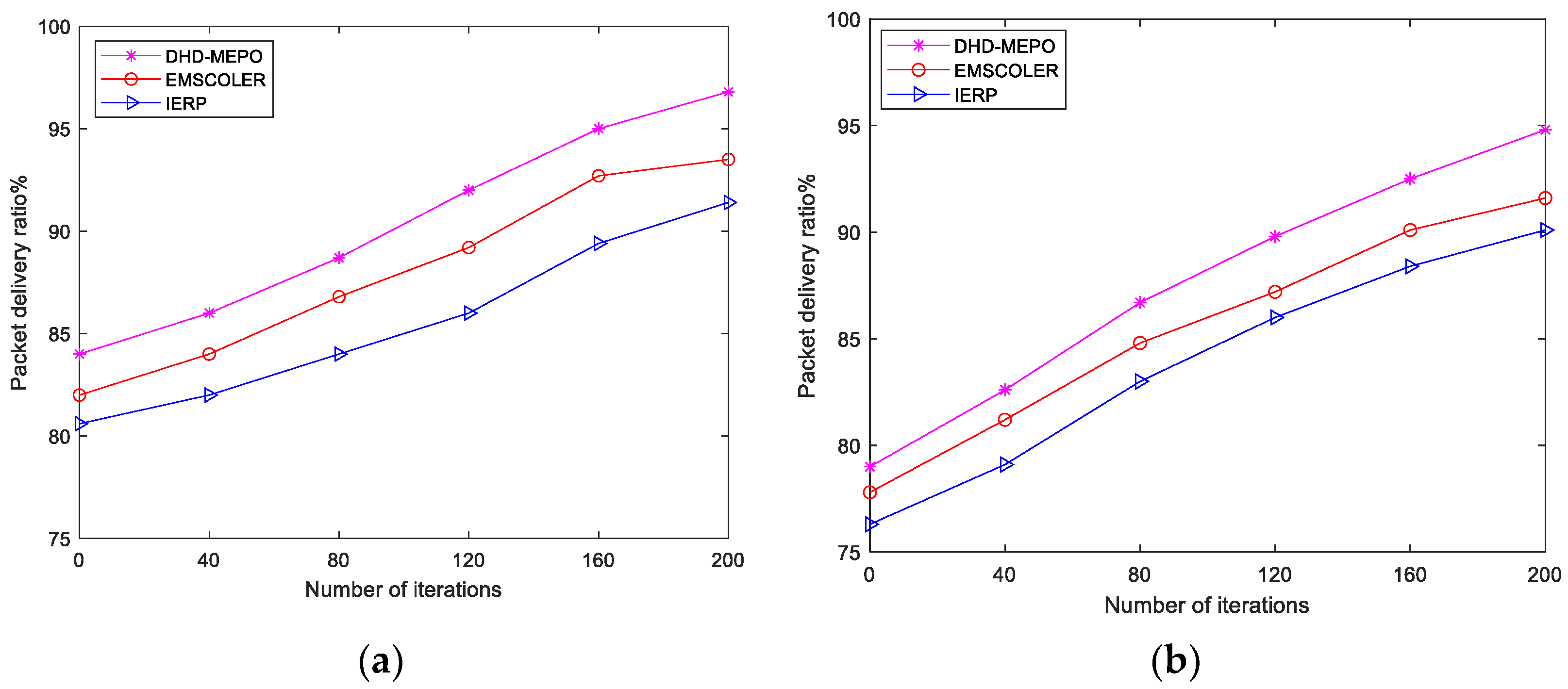
5.6. Packet Delivery Ratio Analysis

We explore the packet delivery ratio of DHD-MEPO versus EMSCOLER and IERP, experimenting for two network environments of each size. The packet delivery ratio is defined as the ratio of the quantity of packets received by the BS to the total quantity of packets sent. The analysis of Figure 19a,b shows that the packet delivery rate using the DHD-MEPO algorithm is always in the leading position. The reason for this is that in the initial stage of the algorithm, the network is divided into cells and group nodes are selected for the group management of the cells, and the group nodes are responsible for collecting and aggregating the data information within the cells they manage before sending it to the BS center for further processing. IERP and EMSCOLER do not take into account this aspect of the packet management network area, but the reason why the packet delivery rate is higher with EMSCOLER than with IERP is that EMSCOLER uses a grid concept and selects relay nodes for data transmission in the steady state of the link.

By comparing it with other algorithms, we demonstrate that DHD-MEPO performs well in the aspect of coverage and uniformity of energy consumption. (1) In the aspect of energy performance, the deficiencies of 3D-VPCA, a derivative algorithm of the Virtual Force Algorithm (VFA), affect the virtual movement of mobile nodes and the energy consumption of the movement. Meanwhile, the C-CICHH’s total energy consumption is slightly worse than that of DHD-MEPO, because C-CICHH transforms it into a maximum weighted exact-match matter by designing a weighted complete dichotomous chart, with the aim of finding the allocation strategy that minimizes the total energy consumption while solving the network coverage problem. Furthermore, 3D-VPCA and C-CICHH only take maximizing coverage and minimizing total energy consumption as the optimization objectives, ignoring the uniformity of the remaining energy of the nodes. In contrast, DHD-MEPO optimizes the remaining energy equalization as the major factor in the process of repairing holes. Therefore, the algorithm in this paper outperforms 3D-VPCA and C-CICHH in the performance of residual energy equalization. (2) In terms of coverage enhancement, the essence of 3D-VPCA and DHD-MEPO is to separate redundant mobile nodes to fill the unmonitored region. However, the final movement effect of the repair nodes in 3D-VPCA will inevitably be affected by the attraction between the nodes and the uncovered points being monitored threshold, the repulsive force threshold between the nodes, as well as the step distance during each round of virtual movement. Although these parameters are iteratively adjusted to ensure optimal performance, the results are not significantly improved. This is the reason why the final coverage after the 3D-VPCA repair is lower than the algorithm in this paper.

6. Conclusions and Future Work

Previous research into coverage holes in wireless sensor networks mainly focus on two-dimensional planar environments, but we propose a detection and repair approach suitable for three-dimensional hybrid wireless sensor networks so as to effectively improve the QoS. The DHD-MEPO is distributed and organized into two parts: detection and repair. In the detection part, the target region is partitioned based on the quantity of nodes distributed and their sensing range. The group nodes are campaigned to manage information about relevant nodes within their own cells, which ensures network stability and lengthens the network lifecycle. The group nodes also count the sources of hole information based on the calculated cell coverage. In the repair part, the set of candidate repair nodes is selected by calculating the redundancy of the mobile nodes to cover the target point. Then, it uses a multi-objective emperor penguin optimization algorithm, which determines the best location for the repair node.

In real scenarios, the sensing range of the sensor node is also affected by environmental changes and multiple obstacle obstructions, as well as the fact that its sensing range is variable over time in complex scenarios. Therefore, in subsequent work, we will take a broader perspective in comparison with advanced work to further validate the advancement of the method in complex underwater or mountainous terrain scenarios.