Improving the Performance of the Single Shot Multibox Detector for Steel Surface Defects with Context Fusion and Feature Refinement

Abstract

Strip surface defects have large intraclass and small interclass differences, resulting in the available detection techniques having either a low accuracy or very poor real-time performance. In order to improve the ability for capturing steel surface defects, the context fusion structure introduces the local information of the shallow layer and the semantic information of the deep layer into multiscale feature maps. In addition, for filtering the semantic conflicts and redundancies arising from context fusion, a feature refinement module is introduced in our method, which further improves the detection accuracy. Our experimental results show that this significantly improved the performance. In particular, our method achieved 79.5% mAP and 71 FPS on the public NEU-DET dataset. This means that our method had a higher detection accuracy compared to other techniques.

1. Introduction

For various reasons, including continuous casting billets and the production equipment and process, strip steel surfaces may have defects, such as surface pitting, rolled scale, scratches, and so on. These defects seriously affect the strip steel quality and may even destroy the subsequent production object. Therefore, the efficient detection of surface defects is pivotal for strip steel production.

Surface defect detection is essentially a kind of target detection, to which various convolutional neural network methods have been applied. Nonetheless, the surface defects of a strip steel differ significantly from other types of target. They are usually characterized by large intraclass and small interclass differences, resulting in the existing convolutional neural network methods failing to achieve a good balance between detection accuracy and efficiency.

To solve this problem, we propose a single-stage target detection method based on the single-shot multibox detector (SSD) [1]. The method consists of three stages, as follows: The first is the feature extraction stage. As the residual structure helps to build a deep network that can extract high-dimensional semantic features, ResNet50 [2] is used as the feature extraction network, and the feature maps extracted from its fourth residual block are sequentially downsampled by five additional layers, to construct five feature maps of different scales to detect defective targets of different sizes.

The second is the encoding stage. A context fusion structure was designed to introduce more contextual information for the multiscale feature maps, which increases the inference speed, while improving the ability of the model to capture defects.

The third is a decoding stage. A feature refinement module is added to the predicted feature map. Via the channel and spatial attention mechanisms, the model is guided to better integrate the context information, which solves the semantic conflict and redundancy caused by the context fusion, and the detection accuracy of the model is thus further improved. Finally, six simple predictors are used to predict the six predicted feature maps, respectively. We evaluated our method with the NEU-DET [3] dataset. The results showed that our method significantly outperformed the other methods. Moreover, our method achieved a better balance between accuracy and efficiency.

We summarize our contributions below:

• We propose a novel method based on the framework of the SSD, which achieves a better balance between detection accuracy and efficiency. For instance, on the NEU-DET dataset, our method achieved an accuracy of 79.5% mAP at a speed of 71 FPS, thereby outperforming other methods.
• We designed a context fusion structure for the framework, which is able to more closely capture the surface defects, while maintaining the inference speed. Our structure is simpler than that in [4,5], as we only use a dilated convolution to transfer location information from the bottom to the top and a deconvolution to transfer semantic information from the top to the bottom.
• We introduced a feature refinement module into the framework, which efficiently rules out the semantic conflicts and redundancies that result from context fusion. This improved the resulting detection accuracy. This idea stemmed from [6,7], where we combine the channel and spatial attention mechanisms for adaptive feature refinement and replace the fully connected layer in channel attention with 1 × 1 convolution.

2. Related Works

Early rolling steel enterprises generally used manual methods to detect defects. These methods obviously had a poor efficiency [8,9,10] and could suffer from poor performance caused by fatigue. However, nondestructive testing technologies have been used to detect surface defects (e.g., ultrasonic flaw detection), these methods present shortcomings, such as a high equipment installation cost and energy consumption and slow detection speed. With the combination of computer technology and vision, detection methods based on machine vision have been proposed [11,12,13,14,15]. However, their defect features need to be manually extracted and the resulting low-dimensional artificial features are difficult to generalize to complex strip surface defects. Therefore, the application of these methods needs to be combined with specific scenarios [15,16].

With the increase of computing power, detection methods based on convolutional neural networks have gradually become mainstream and can mainly be divided into two categories: The first is a two-stage target detection method, and the second is a single-stage target detection method. The two-stage target detection method includes a region proposal stage and a target bounding box regression and classification stage. While this has high accuracy, it generally has slow inference, because of its complex structure. Typical examples include the RCNN [17], Fast R-CNN [18], and Faster R-CNN [19]. The single-stage target detection method has a higher inference speed and integrates these two stages into an end-to-end network. Thus, its accuracy is slightly lower than that of a two-stage target detection method. Typical examples of single-stage target detection methods include the SSD [1], RetinaNet [20], YOLOv3 [21], YOLOv4 [22], YOLOv5 [23], YOLOX [24] and so on.

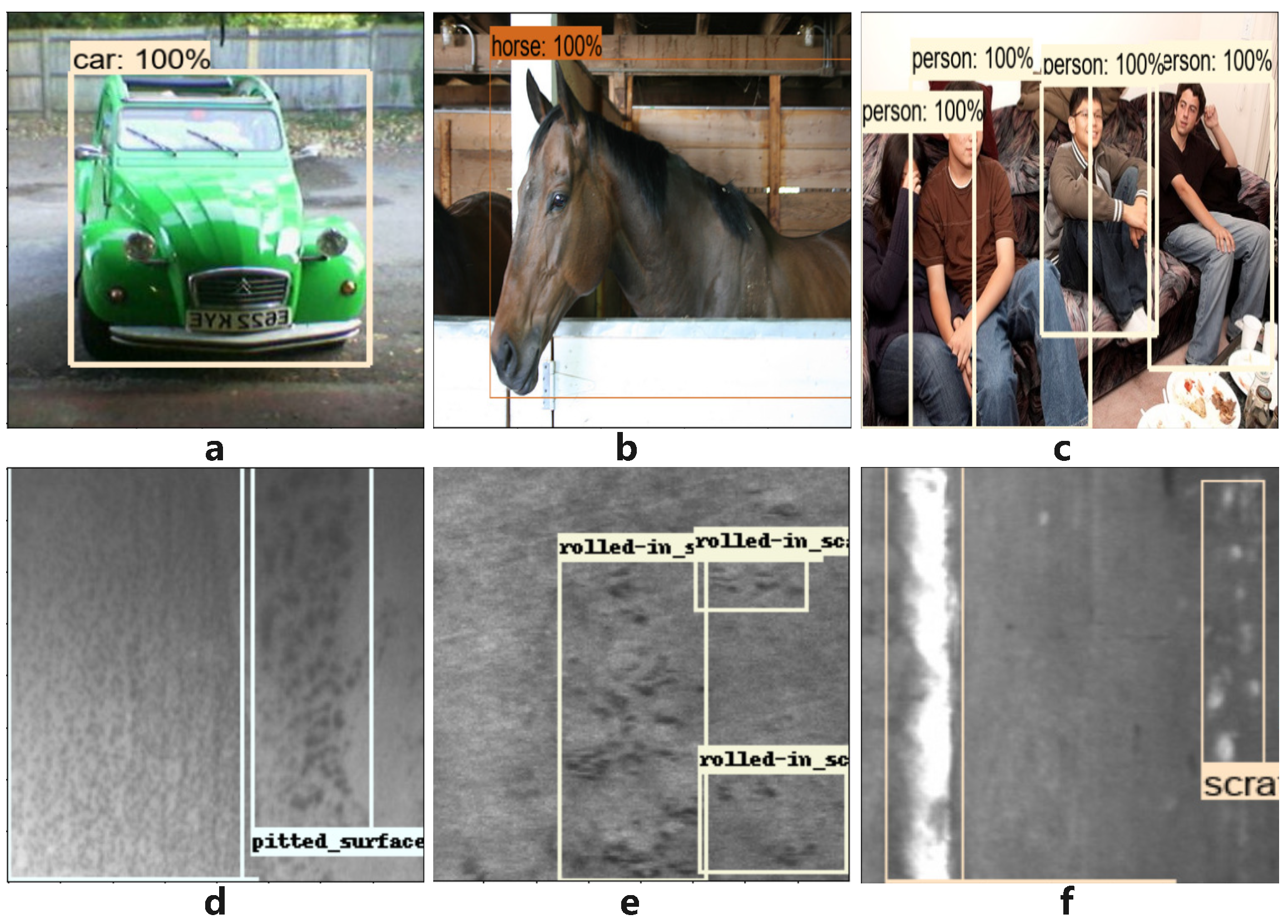
Since surface defects are characterized by large intraclass and small interclass differences, these classic target detection methods cannot usually be applied directly, as the targets in applications differ significantly from the surface defects in this study, as shown in Figure 1.

While these classic methods cannot be applied directly, they provide deep insights for detecting the surface defects of strip steel. We direct the readers to references [25,26,27,28,29] for detailed introductions to these methods.

To improve the performance of the Faster-RCNN in surface defect detection, Zhao et al. [25] proposed a refined Faster-RCNN method, which is a two-stage target detection model that first extracts the target region with a RPN network and achieved 75% mAP on the NEU-DET dataset. While this performance is excellent, the detection speed is still slow and insufficient to cope with practical demands. Moreover, Hatab et al. [26] designed a defect detection method based on the YOLO network and obtained 70.66% mAP on the NEU-DET dataset. Thereafter, Kou et al. [27] proposed a defect detection model based on anchor-free YOLO-v3 and achieved 72.2% mAP. He et al. [28] then proposed a two-stage defect detection model based on multifeature map fusion and achieved 82.3% mAP. However, when the model increased the detection speed to 20 FPS, the mAP dropped to 70%. In addition, Cheng et al. [29] recently proposed a single-stage defect detection method based on RetinaNet, which exhibited 78.25% mAP. Although the accuracy has been improved with these models, their detection speed cannot meet the requirements of an actual production line.

While there are various methods for strip surface defect detection, they are still unable to achieve a good balance between detection accuracy and efficiency. Thus, this remains an open technical problem. The method proposed in this study provides insights into this challenge, by achieving a good balance when using the NEU-DET dataset.

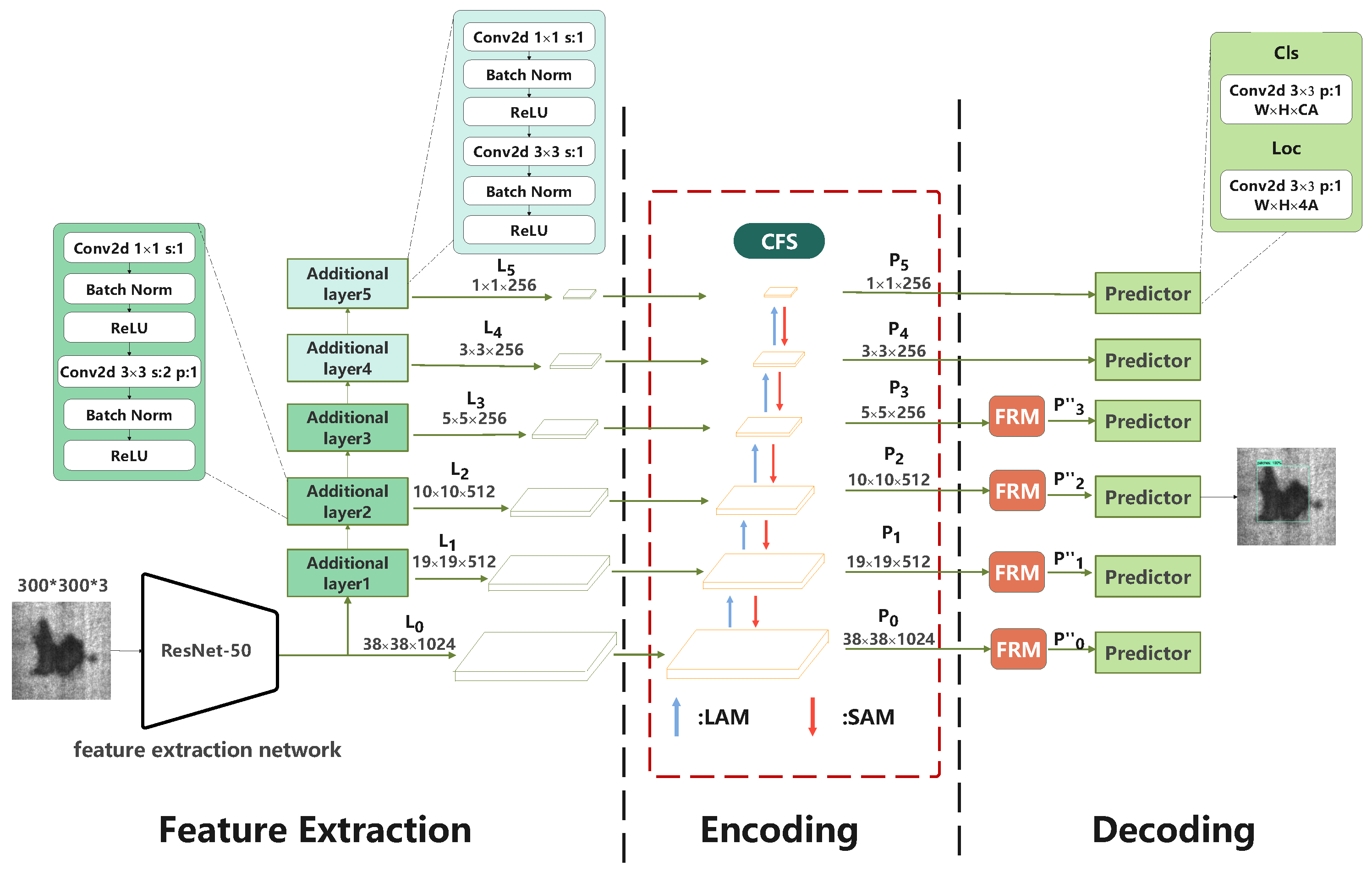
3. Model

We use the SSD as the overall framework. Compared to the Faster R-CNN, RetinaNet, YOLOv3, YOLOv4, YOLOv5, YOLOX, and so on, the SSD has a simple structure and fast detection speed. In particular, it is easy to deploy and integrate with industrial equipment.

Our model consists of three stages. The first stage is a feature extraction stage, which includes a feature extraction network with additional layers, as shown in Figure 2. From this network, six feature maps of different scales can be obtained ($L_0$∼$L_5$ layer feature maps in Figure 2). The second stage is a coding stage, which builds a context fusion structure (CFS) based on six feature maps and introduces more contextual information into the model through a location augmentation module (LAM) and semantic augmentation module (SAM), to obtain the final predicted feature maps ($P_0$∼$P_5$ layer feature maps in Figure 2). The third stage is a decoding stage, which adds a feature refinement module (FRM) after the first four predicted feature maps ($P_0$∼$P_3$ layer feature maps in Figure 2), to filter out the semantic conflicts and redundancy caused by contextual feature fusion. Finally, we use six predictors to regress the offset of the defect target location and classify the defect targets.

3.1. Feature Extraction Stage

The feature extraction stage first extracts a high-dimensional feature map from a 300 × 300 image using a feature extraction network and then obtains five different scales of feature maps ($L_1$∼$L_5$ layer feature maps in Figure 2) using five additional layers on this high-dimensional feature map, before finally sending this to the encoding stage. It should be noted that we use ResNet50 [2] instead of VGG16 [30] in the feature extraction network. ResNet50 is better than VGG16 in terms of its computational power and characterization ability. We only use the first seven layers of ResNet50 as the feature extraction network. Moreover, we refer readers to NVIDIA’s code (available online at https://github.com/NVIDIA/DeepLearningExamples/tree/master/PyTorch/Detection/SSD (accessed on 8 December 2021)), where the stride of the first residual block of the Conv-4x layer is modified to 1 to improve the resolution.

Although multiscale feature maps can improve the performance for detecting targets of different sizes, these predictive feature maps ($L_0$∼$L_5$ layer feature maps in Figure 2) can only be obtained with a series of additional layers of recursive relationships on top of the feature extraction network. Therefore, they differ only in the size of the receptive fields and cannot make good use of the multiscale features, whose receptive field sizes are defined as:

$$R_{\mathit{L}}=R_{\mathit{L}-1}+\left[F_{\mathit{L}-1}\times \prod _{i=1}^{L-1}{S}_i\right]$$

(1)

where L represents the number of layers ($0\le L\le 5$); $R_L$ denotes the receptive field size of the $L_{th}$ layer, which is related to the receptive field size of the preceding layer; $F_L$ denotes the size of the pooling or convolution kernel of the L-th layer; and $S_i$ denotes the stride of the $i_{th}$ layer.

According to the definition of the receptive field size, we assume that the receptive field size of the $L_0$ layer is 1. We can then derive the receptive field expansion multipliers of the feature maps extracted from the additional layers ($L_1$∼$L_5$ layer feature maps in Figure 2), as shown in

Table 1. Expansion of receptive field relative to the $L_0$ layer.

Feature Map	${\mathit{L}}_1$	${\mathit{L}}_2$	${\mathit{L}}_3$	${\mathit{L}}_4$	${\mathit{L}}_5$
Multiplier	4	10	22	40	58

. It can be seen that the receptive field size of the last layer is 58-times larger than that of the first layer and it can therefore extract richer and more concise semantic features compared to the $L_0$ layer and detect large targets better. However, it also weakens the ability to perceive more local information compared to the $L_0$ layer, thus influencing the detection of small targets.

3.2. Encoding Stage

As shown in Section 3.1, the $L_0$∼$L_5$ layer feature maps do not make good use of the contextual information. For this, Fu et al. [4] used deconvolution and skip connections on the basis of SSD to transfer the semantic information of deep layers to shallow layers using element-wise multiplication. Meanwhile, Jeong et al. [5] not only used deconvolution to directly connect the semantic information of deep layers with the shallow feature map in a stacked manner in the channel dimension, but also used the pooling layers to stack the local information of shallow layers to the deep feature map in the same way.

To introduce context information, our method not only transfers the semantic information of deep layers to shallow layers, but also transfers the local information of shallow layers to deep layers. At the same time, in the process of transmitting local information, we do not use pooling layers, as in [5], but replace them with dilated convolution.

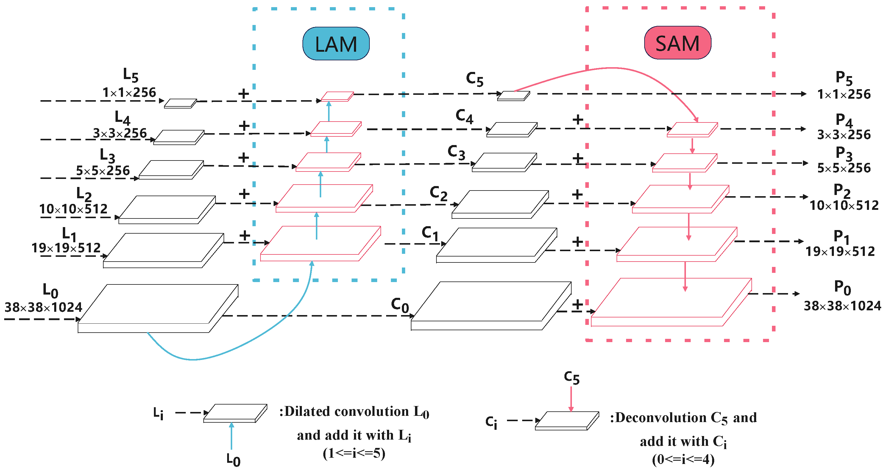
We therefore designed a CFS that contains a LAM and a SAM, as shown in Figure 3. The CFS fuses the rich and concise semantic information in the deep layer together with the relatively accurate local position details in the shallow layer into the predicted feature map. This improves the ability to capture the surface defects, while maintaining the inference speed.

As shown in Figure 3, the LAM transfers the relatively accurate local position information in the $L_0$ layer to the deep layer. This makes the feature map size of the $L_0$ layer consistent with the $L_1$ layer through a downsampling operation. The $L_1$ layer then joins to obtain the $C_1$ layer. After that, the $L_0$ layer continues to downsample and the $L_2$ layer joins to obtain $C_2$. By repeating this, we eventually obtain $\{C_3$∼$C_5\}$. Note that the $C_0$ layer is obtained by the $L_0$ layer without any other operations. Although traditional downsampling (pooling or convolution) can increase the receptive field, it might raise the problem of spatial resolution degradation, which does not transfer the rich position information of the $L_0$ layer to subsequent layers well. Therefore, we use dilated convolution with kernels of size $3\times 3$, a stride size of 2, and a dilation rate of 2 for downsampling. For the last two downsampling operations, the stride size is adjusted to 1, since the feature map is small and a larger stride size may lead to information loss.

The SAM transfers the rich and concise semantic information from the $C_5$ layer to the shallow layer, which makes the feature map size of the $C_5$ layer consistent with the $C_4$ layer through a upsampling operation. The $C_4$ layer is then summed, to obtain the $P_4$ layer, after which the $C_5$ layer continues to be upsampled and summed with the $C_3$ layer to obtain the $P_3$ layer. By repetition, we eventually obtain $\{P_0$∼$P_2\}$. Note that the $P_5$ layer is obtained from the $C_5$ layer without any operations. Here, we do not use the same nearest-neighbor upsampling as the feature pyramid network [31]. In its place, a deconvolution operation with learning capability is applied, which has a stronger ability to reduce the resolution than nearest-neighbor upsampling and has shown effectiveness in detection and segmentation [4,32,33,34]. All deconvolution kernels have a size of $3\times 3$ and a stride size of 2. For the first two upsampling operations, we use a stride size of 1.

3.3. Decoding Stage

The decoding stage contains a FRM and a predictor. After passing through the FRM, the predicted feature maps are fed into six predictors that do not share parameters and are independent. Here, each predictor contains two branches. One is for regressing the offset of the defect target location and the other classifies the defect target.

In context fusion, although the CFS introduces more contextual information for predicting feature maps, directly fusing feature information of different scales will result in semantic conflicts. This reduces the characterization ability of multiscale feature maps and influences the resulting defect detection.

For this, Woo et al. [6] used an spatial attention mechanism and a channel attention mechanism for adaptive feature refinement. However, in the channel attention mechanism, two of these fully connected layers were used as features after average pooling and maximum pooling, to learn a set of mappings. At the same time, in order to reduce the parameters of the fully connected layers, the dimensions of these two fully connected layers were reduced. In [7], it was found that the dimensionality reduction of these fully connected layers had a negative impact on the channel attention mechanism, and $1\times 1$ convolution was used to solve this problem.

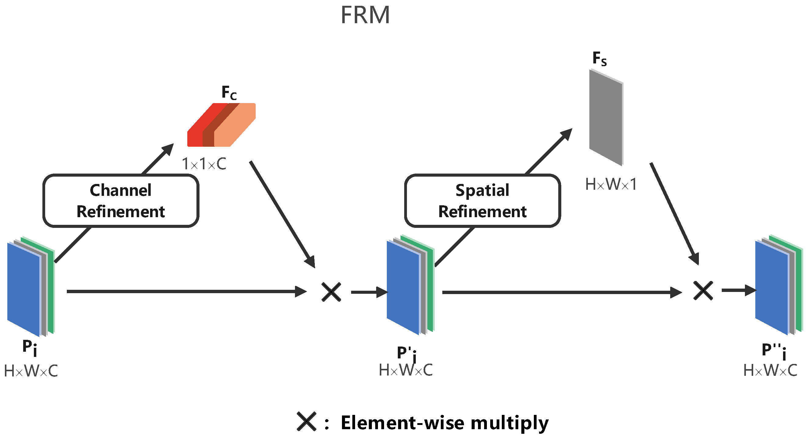
Inspired by CBAM [6] and ECANet [7], we add a FRM after $\{P_0$∼$P_3\}$ to refine the channel and spatial information of the predicted feature maps fused with the contextual information, and use $1\times 1$ convolution to replace the fully connected layers in the channel attention mechanism, so as to guide the contextual fusion and filter out the semantic conflicts and redundancies brought by direct information fusion of different scales.

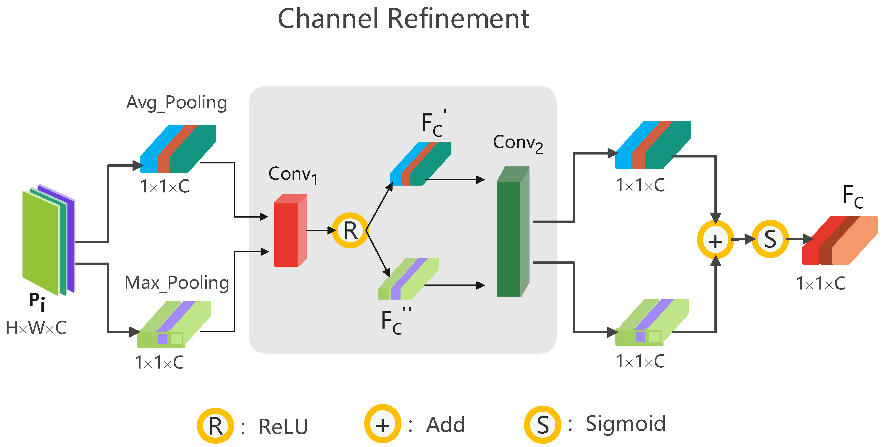
As shown in Figure 4, given the prediction feature map $P_i\in R^{H\times W\times C},(0\le i\le 3)$ as input, the channel and spatial refinements $F_c\in R^{1\times 1\times C}$ and $F_s\in R^{H\times W\times 1}$ are obtained in turn and then the final prediction feature map $P_i^{″}\in R^{H\times W\times C}$ using the following steps:

$$P_i^{\prime }=F_c\times P_i$$

(2)

$$P_i^{″}=F_s\times P_i^{\prime }$$

(3)

where × is the element-wise multiplication, and $F_c$ and $F_s$ can be regarded as weights in the channel and space dimensions, respectively.

As shown in Figure 5, channel feature refinement uses the channel attention mechanism to obtain the weights of the feature maps, so that the model gives more attention to the information that should be learned and filters out the semantic conflicts and redundancies. Given a prediction feature map $P_i\in R^{H\times W\times C},(0\le i\le 3)$ as input, the feature map is squeezed into two feature longs with dimensions $1\times 1\times C$ by global average and global maximum pooling operations, respectively. These two feature longs are then fed into $Con{v}_1$ with a convolution kernel size of $1\times 1$, compressing its channel number to $C\times \frac{1}{ratio}$, and activated by the activation function $\varphi :ReLU\left(\right)$ to obtain $F_c^{\prime }\in R^{1\times 1\times C\times \frac{1}{ratio}}$ and $F_c^{″}\in R^{1\times 1\times C\times \frac{1}{ratio}}$:

$$F_c^{\prime }=\varphi \left(Con{v}_1\left(AvgPooling\left(P_i\right)\right)\right)$$

(4)

$$F_c^{″}=\varphi \left(Con{v}_1\left(MaxPooling\left(P_i\right)\right)\right)$$

(5)

Finally, $F_c^{\prime }$ and $F_c^{″}$ are fed into $Con{v}_2$ with a convolution kernel of size $1\times 1$ and their channel numbers are reduced back to $1\times 1\times C$. These two are then summed to obtain $F_c\in R^{1\times 1\times C}$ using the activation function $\theta :Sigmoid\left(\right)$:

$$F_c=\theta (Con{v}_2\left(F_c^{\prime }\right)+Con{v}_2\left(F_c^{″}\right))$$

(6)

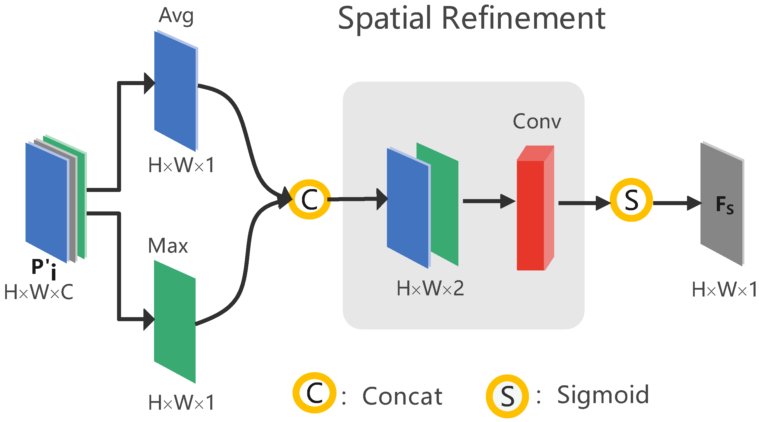
As shown in Figure 6, the spatial feature refinement uses a spatial attention mechanism to obtain the weights of the feature maps in the spatial dimension, so that the model gives more attention to the information learned in the spatial dimension and filters out the semantic conflicts and redundancies brought by the direct fusion of the feature maps in the spatial dimension. Given a prediction feature map $P_i^{\prime }\in R^{H\times W\times C},(0\le i\le 3)$ as input, this is squeezed into two eigenfaces of dimensions $H\times W\times 1$ using an averaging operation and a maximizing operation in the channel dimension, respectively. Moreover, the process stacks them together in the channel dimension, restores the number of channels using a convolution kernel of size $3\times 3$, and then activates them again using $\theta :Sigmoid\left(\right)$ to obtain $F_s\in R^{H\times W\times 1}$:

$$F_s=\theta \left(Conv\left(Concat(Avg\left(P_i^{\prime }\right),Max\left(P_i^{\prime }\right))\right)\right)$$

(7)

4. Experiments

4.1. Experimental Settings and Dataset

4.1.1. Experimental Platform

Pytorch v1.7, 4-core CPU and 2 NVIDIA RTX 3090 GPUs.

4.1.2. Training Parameter Setting

The input image size was $300\times 300$ and the total iteration number was set at 1500. The first 500 iterations were trained by freezing the feature extraction layer and the additional layer, with a batch setting of 8 and a learning rate of 0.01. We then thawed the additional layer for another 500 training sessions, with a batch setting of 16 and a learning rate of 0.001. Finally, we thawed the feature extraction layer for global fine-tuning training, with a batch setting of 32 and a learning rate 0.0001. To optimize the training process, the momentum method was used, with a momentum parameter of 0.9 and a weight decay parameter of 0.3. The decay frequency was once per 30 iterations. To prevent overfitting, image augmentation methods, such as random cropping and flipping, were also used.

4.1.3. Evaluation Metrics

In classification tasks, Params is the total number of parameters that need to be trained during model training, and floating point operations (FLOPs) were used to measure the computational performance of the model, with the smaller the better. Accuracy was used to measure the prediction accuracy of the model, as shown in

Table 2. Model prediction results.

		True Value
		Positive	Negative
Predicted value	Positive	TP	FP
	Negative	FN	TN

. Taking the classification result of the binary classification model as an example, the calculation formula of accuracy was as follows:

$$Accuracy=\frac{TP+TN}{TP+TN+FP+FN}$$

(8)

For the target detection task, not only the classification accuracy, but also the accuracy of the target frame positioning must be considered. This study considered the IoU coincidence degree between the target frame predicted by the model and the real frame as a measure. When the IoU threshold between the target frame and the real frame was greater than 0.5, the model prediction was positive (TP); otherwise, it was negative (TP). The precision and recall were then calculated as follows:

$$Precision=\frac{TP}{TP+FP}$$

(9)

$$Recall=\frac{TP}{TP+FN}$$

(10)

Precision and recall were then calculated according to different classification probabilities, by taking recall as the abscissa and precision as the ordinate and plotting the obtained values to obtain the P-R curve. The area under this curve is the average precision (AP). Finally, the mAP was obtained by averaging the AP of each class.

4.1.4. Dataset

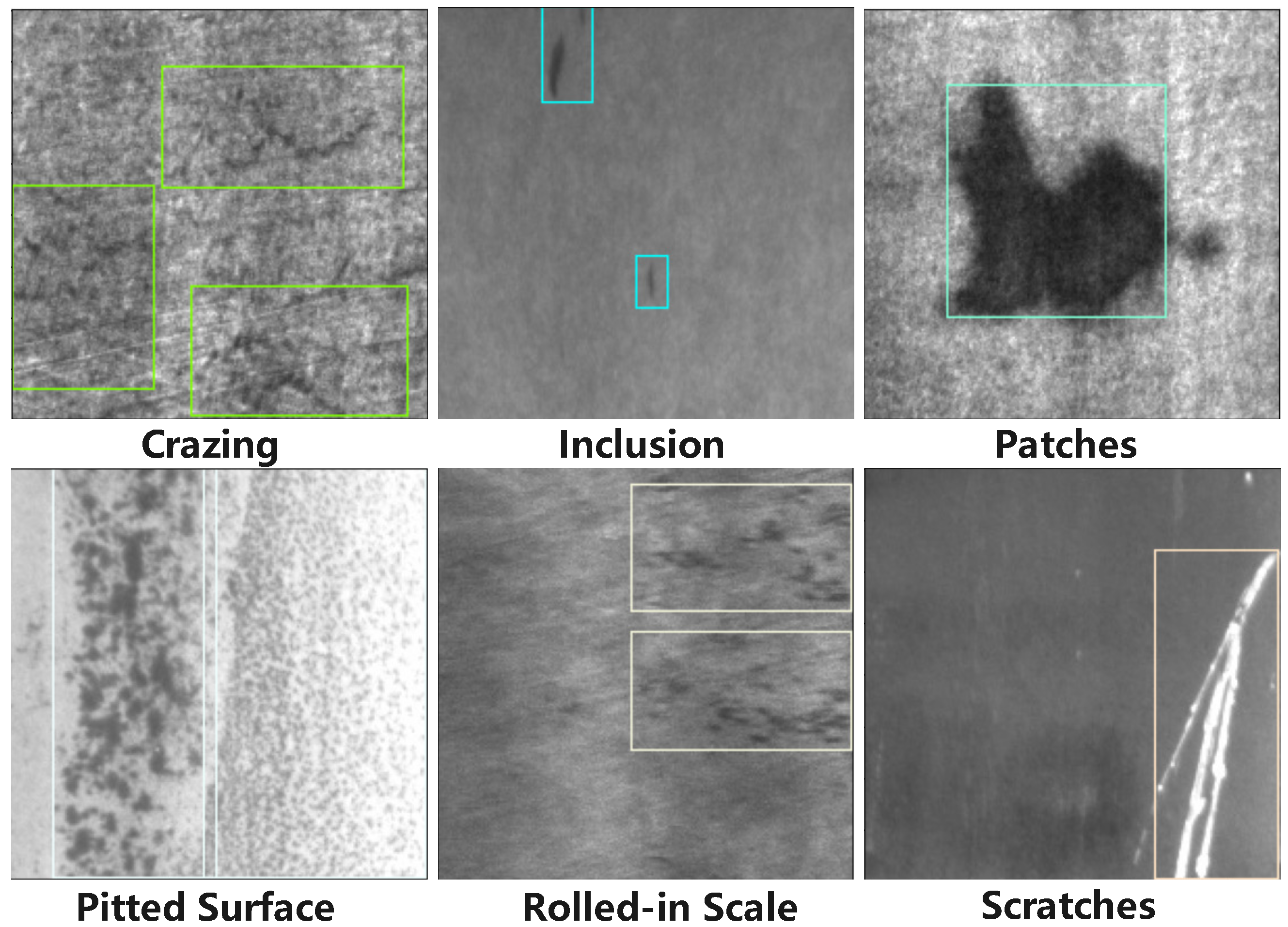
We used the NEU-DET [3] steel surface defect detection dataset created by Northeastern University, China. As shown in Figure 7, this dataset contains six types of hot-rolled strip steel surface defects; namely, crazing (Cr), inclusion (In), patches (Pa), pitted surface (Ps), rolled-in scale (Rs), and scratches (Sc). Each of these classes has 300 images. The dataset thus has 1800 images in total. For each target detection task in this study, we randomly chose 80% of the images as the training set (i.e., 1440 images) and 20% of the images as the test set (i.e., 360 images).

4.1.5. Experiment Design

Our experiment consisted of three steps. In first step, we used an extensive experimental study to show why we used ResNet50 as our feature extraction network. The corresponding experiment results are reported in Section 4.2.

We then report the experimental performance of our framework in Section 4.3. The results showed that our framework outperformed the other methods in detection accuracy and efficiency.

In the third step, we reported a more detailed comparison with other methods. The corresponding experiment showed that our method achieved a much better average performance (Section 4.4).

Finally, we performed an ablation experiment. In our ablation analysis, we showed the impacts of distinct components of the CFS and FRM on the performance of our framework. With this experiment, we eventually chose dilated convolution and deconvolution as the respective downsampling and upsampling methods, and used element-by-element addition to fuse the two feature maps, which, together with FRM and a compression ratio of 32 in layers $P_0$∼$P_3$, achieved an optimal balance between the detection accuracy and efficiency. The details regarding the ablation experiment are presented in Section 4.5.

4.2. Selection of Feature Extraction Network

A good feature extraction network is very important for the performance of a defect detection model. We divided the NEU-DET dataset, according to the defect categories, into six classes, with 10% of the images in each class selected for the test set. This resulted in a steel defect classification dataset with 1620 images in the training set and 180 images in the test set. Different classification models were then applied to classify this steel defect classification dataset, and all models were trained using weights loaded with pretrained weights on the ImageNet [35] dataset. The results are shown in

Table 3. Performance of the different classification models.

Models	VGG16 [30]	Resnet50 [2]	Resnet101 [2]	Resnetxt50 [36]
Accuracy(%)	97.2	100	99.4	98.9
Params(M)	138.36	25.56	44.5	25.03
FLOPs(G)	15.61	4.14	7.87	4.29

. Only Resnet50 [2] achieved 100% accuracy. Although Params was 0.53M larger than Resnetxt50 [36], it had the smallest computational effort (FLOPs).

We used Resnet50 and VGG16 for the feature extraction network, where the details are described in Section 3.1 for Resnet50 and in the original study of the SSD [1] for VGG16.

Table 4. Depth of feature maps composed of VGG and Resnet.

	${\mathit{L}}_0$	${\mathit{L}}_1$	${\mathit{L}}_2$	${\mathit{L}}_3$	${\mathit{L}}_4$	${\mathit{L}}_5$
Resolution	$38\times 38$	$19\times 19$	$10\times 10$	$5\times 5$	$3\times 3$	$1\times 1$
VGG	13	20	22	24	26	27
Resnet50	41	43	45	47	49	51

shows the depths of the feature maps (i.e., the $L_0$∼$L_5$ layer feature maps in Figure 2) in the network derived from the feature extraction stage. Here, only the convolutional and pooling layers were considered when we calculated the depths. The results show that the feature map had the deepest network depth at the same resolution while using Resnet50. This means that the semantic information characterized by Resnet50 was stronger than VGG16, while the improvement in the prediction performance was greater.

In summary, both the Params and FLOPs of Resnet50 were smaller, and the resulting semantic information at the same resolution was stronger. Thus, we used Resnet50 in this study as the feature extraction network.

4.3. Detection Performance of the Model

4.3.1. Detection Accuracy of Model

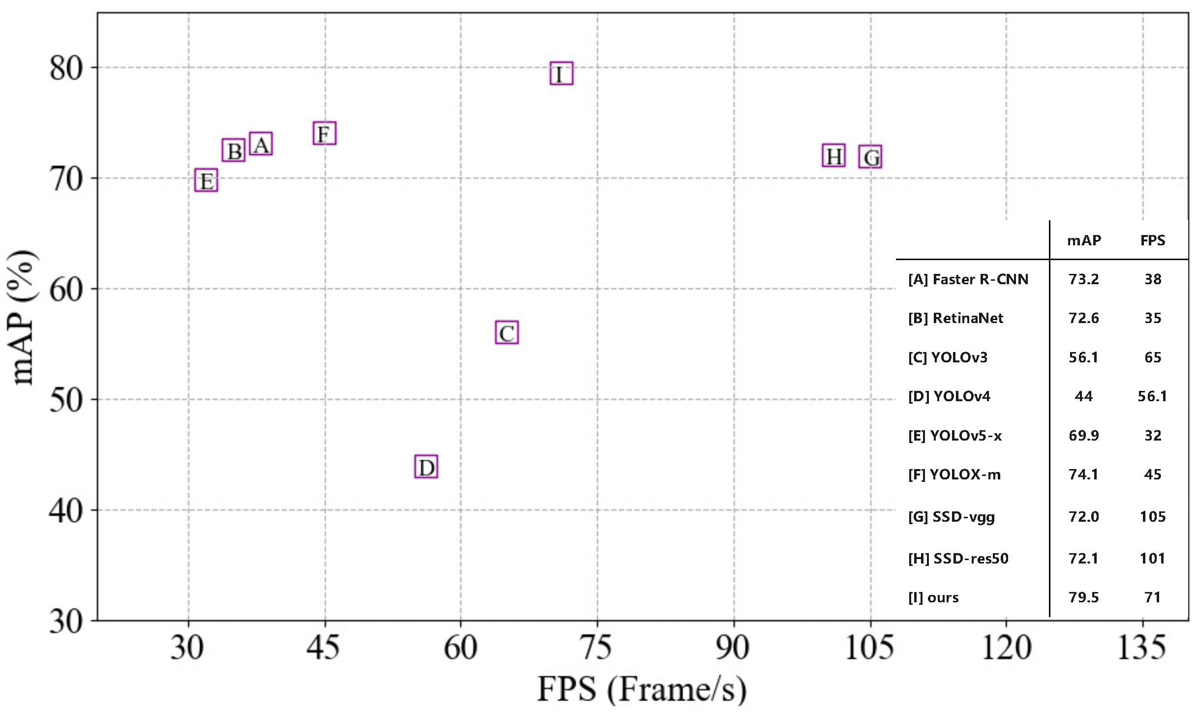
As mentioned above, we used the SSD as the overall framework and Resnet50 as the feature extraction network. In addition, a CFS was used in the encoding stage to introduce more contextual information into the multiscale feature map. This ensured a higher inference speed and improved the characterization ability of the multiscale feature map. Furthermore, in the decoding stage, in order to filter out the semantic conflicts and redundancies brought by feature fusion, a FRM was added after the first four layers of predicted feature maps, to further improve the detection accuracy. The results are shown in Figure 8.

Our model achieved 79.5% mAP and 71 FPS on the NEU-DET dataset. Our accuracy outperformed those of SSD-resnet50 and SSD-vgg16 at rates of 7.4/72.1 and 7.5/72.0, respectively. Compared to the other methods, our model achieved the best accuracy (mAP) and had a sufficient detection speed (FPS).

4.3.2. Efficiency

The inference of the image, including the execution of non-maximum suppression, took only 0.014 s and the detection speed reached 71 FPS. In a real production line, a single camera has a range of 50–100 cm and the maximum production speed is usually 30 m/s, which requires a detector speed of at least 30∼60 FPS [37]. Therefore, the detection speed of our model meets such requirements of practical applications.

4.4. Detailed Comparison with Other Models

To further evaluate its effectiveness, we compared our model with several existing methods using the NEU-DET dataset. For a comprehensive comparison, we considered both two- and single-stage target detection methods. We used Faster R-CNN [19] as an example two-stage target detection method, which uses a region proposal network to generate candidate target frames. For the single-stage target detection method, we chose RetinaNet [20] configured with the feature pyramid network and different YOLO methods, namely YOLOv3 [21], YOLOv4 [22], YOLOv5 [23], YOLOX [24], YOLOv8 [38], and SSD [1]. The comparison results are shown in

Table 5. Comparison results with other models.

Methods	Backbone	mAP(%)	FPS	Cr(%)	In(%)	Pa (%)	Ps(%)	Rs(%)	Sc(%)
Faster R-CNN [19]	Resnet50+FPN	73.2	38	33	79	92	84	54	95
RetinaNet [20]	Resnet50+FPN	72.6	35	38	78	94	85	54	84
YOLOv3 [21]	Darknet53	67.4	65	29	73	89	79	50	85
YOLOv4 [22]	CSPDarknet53	23.9	44	5	24	43	46	5	20
YOLOv5-s [23]	CSPDarknet	59.6	68	17	72	86	68	37	77
YOLOv5-m [23]	CSPDarknet	63.8	50	19	73	89	75	46	81
YOLOv5-l [23]	CSPDarknet	69.6	44	32	75	91	75	58	88
YOLOv5-x [23]	CSPDarknet	69.9	32	28	76	92	76	57	90
YOLOX-s [24]	CSPDarknet	71.2	60	35	73	92	82	56	90
YOLOX-m [24]	CSPDarknet	74.1	45	38	80	91	84	57	96
YOLOX-l [24]	CSPDarknet	73.8	41	39	76	92	86	57	93
YOLOX-x [24]	CSPDarknet	73.5	30	37	78	93	84	58	93
YOLOv8-n [38]	CSPDarknet	72.0	144	33.7	78.1	89.9	79.7	56.7	93.6
YOLOv8-s [38]	CSPDarknet	69.8	116	28.0	74.8	89.9	80.6	54.5	91.0
YOLOv8-m [38]	CSPDarknet	71.8	103	35.6	78.1	91.2	77.6	57.3	91.1
YOLOv8-x [38]	CSPDarknet	72.3	56	35.9	77.8	90.8	79.3	59.5	90.2
SSD [1]	VGG16	72.0	105	37	76	91	86	61	77
SSD	Resnet50	72.1	101	37	76	91	81	60	86
Ours	Resnet50	79.5	71	48	82	94	86	73	92

. Compared to these existing methods, our model again achieved the best accuracy. Moreover, the detection speed was only poorer than the SSD and YOLOv8.

4.5. Ablation Experiments

Finally, we conducted ablation experiments for further evaluation of the CFS and FRM.

4.5.1. CFS

The CFS involves information fusion of two feature maps of different sizes and needs to use upsampling and downsampling to adjust the sizes of the feature maps. We designed two different strategies for upsampling and downsampling. One was dilated convolution and deconvolution with a LAM and a SAM, as discussed in Section 3.2. These are self-adaptive and so can optionally fuse two feature maps during training. The other was a combination of a LAM-S and a SAM-S. As in the method in [5], the LAM-S uses a maximum pooling as downsampling, so as to pass the local position detail information to the rest of the layers. The SAM-S uses a nearest neighbor interpolation as upsampling, to pass the semantic information to the rest of the layers. In addition, we needed a suitable fusion approach to fuse feature maps after their sizes become identical. 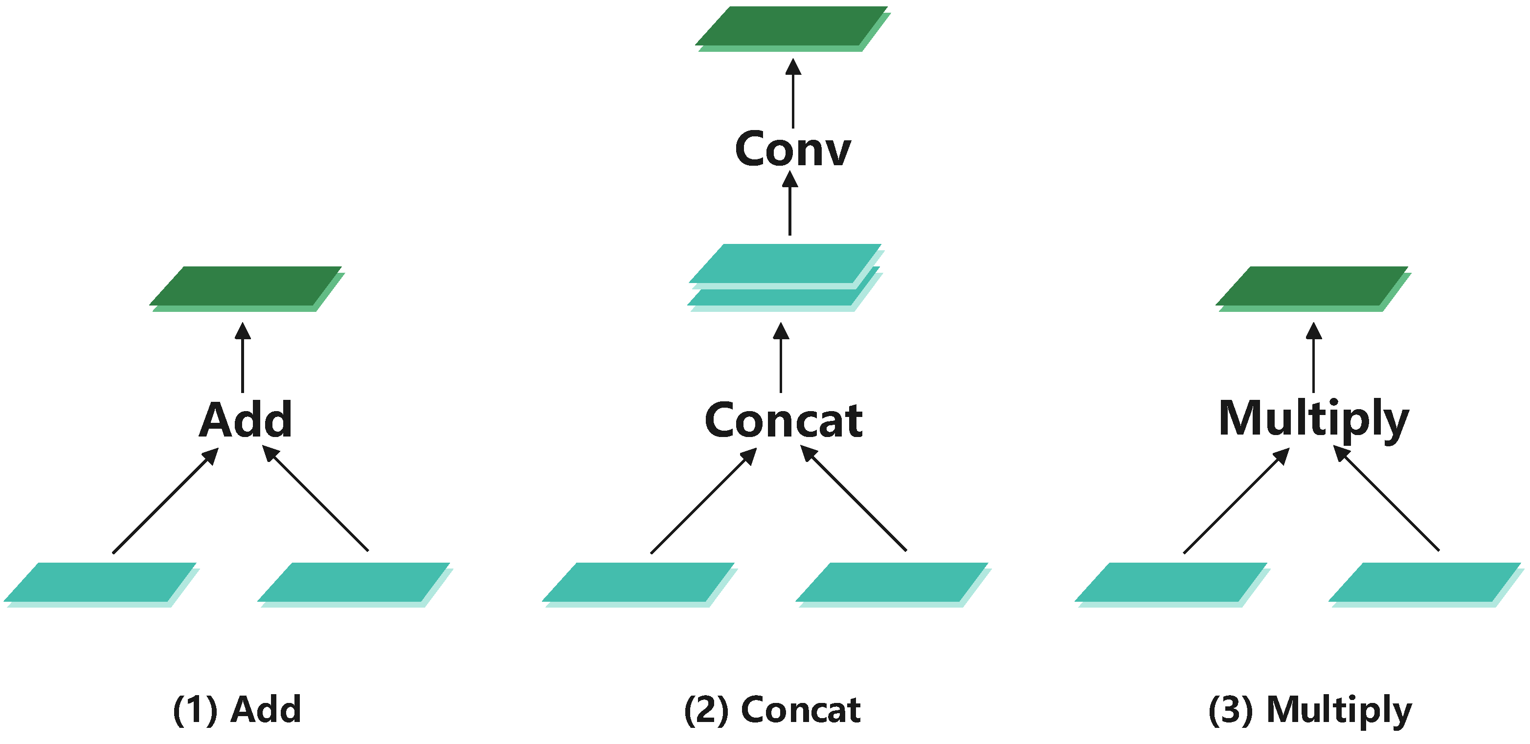Figure 9 shows the performance of three fusion methods in the CFS. The first was element-by-element addition (Add) fusion. The second was element-by-element multiplication (Multiply) fusion. The third stacks two feature maps in the channel dimension and then downscales them to the original channel number using $1\times 1$ convolution and is usually shorted as Concat.

Table 6. Three types of feature map fusion and two strategies of downsampling and upsampling. ✓ represents the use of this module.

Module	Add	Concat	Multiply	mAP
LAM	✓			76.8
LAM		✓		55.0
LAM			✓	76.5
LAM-S	✓			75.7
LAM-S		✓		71.6
LAM-S			✓	39.3
SAM	✓			76.2
SAM		✓		47.5
SAM			✓	73.9
SAM-S	✓			55.7
SAM-S		✓		46.2
SAM-S			✓	53.4

shows the experimental results. Add achieved the best performance for both upsampling and downsampling. Furthermore, the performance of LAM and SAM was better than the LAM-S and SAM-S. Hence, the combination of Add with upsampling and downsampling with a learning capability was a good choice.

We eventually choose the combination of Add with LAM and SAM as the two optional components of the CFS.

Table 7. Components of the CFS module. ✓ represents the use of this module.

LAM	SAM	mAP	FPS
		72.1	101
✓		76.4	90
	✓	76.2	91
✓	✓	78.5	89

shows the resulting effectiveness of the four possible combinations of these two components in terms of mAP and FPS.

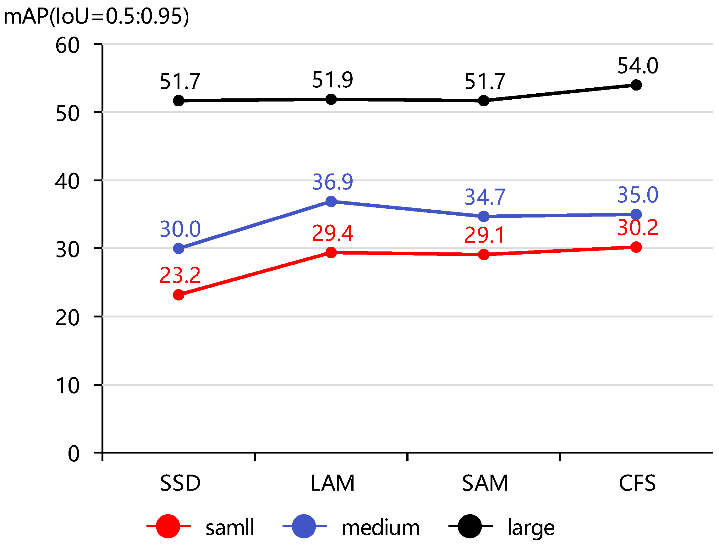
Without the LAM and SAM, our method degenerated to the baseline model SSD-resnet50, which had a detection accuracy of 72.1 mAP on the NEU-DET dataset. With only the LAM or the SAM, the detection accuracy was improved by 4.3 and 4.1 percentage points, respectively. Moreover, the LAM improved the performance more significantly, especially for small instances, see, for example, Figure 10.

When the LAM and SAM were used together, the mAP was improved by 6.4 percentage points compared to the baseline model and the detection accuracy of small targets was improved by 7 percentage points. This means that introducing contextual information into the prediction feature maps indeed improved the detection accuracy, especially for small targets. In particular, the inference speed reached 89 FPS and was still comparable with that of the baseline model.

4.5.2. FRM

Our model used the CFS to introduce more contextual information to the multiscale feature map, to improve its detection capability. Then, we validated the effectiveness of the FRM in filtering out semantic conflicts and redundancies.

Table 8. CFS and FRM modules. ✓ represents the use of this module.

CFS	FRM	CBAM	mAP	FPS
			72.1	101
✓			78.5	89
✓		✓	75.6	71
✓	✓		79.5	71

shows that we obtained a 1 percentage point improvement when we combined the CFS with the FRM. This achieved a 7.4 percentage point improvement compared to the baseline model (without the CFS and FRM).

We also implemented a comparative experimental study to show the effectiveness of using $1\times 1$ convolutional layers to replace the fully connected layers in CBAM, see the results in Table 8. With $1\times 1$ convolution, the detection accuracy of our model was considerably improved.

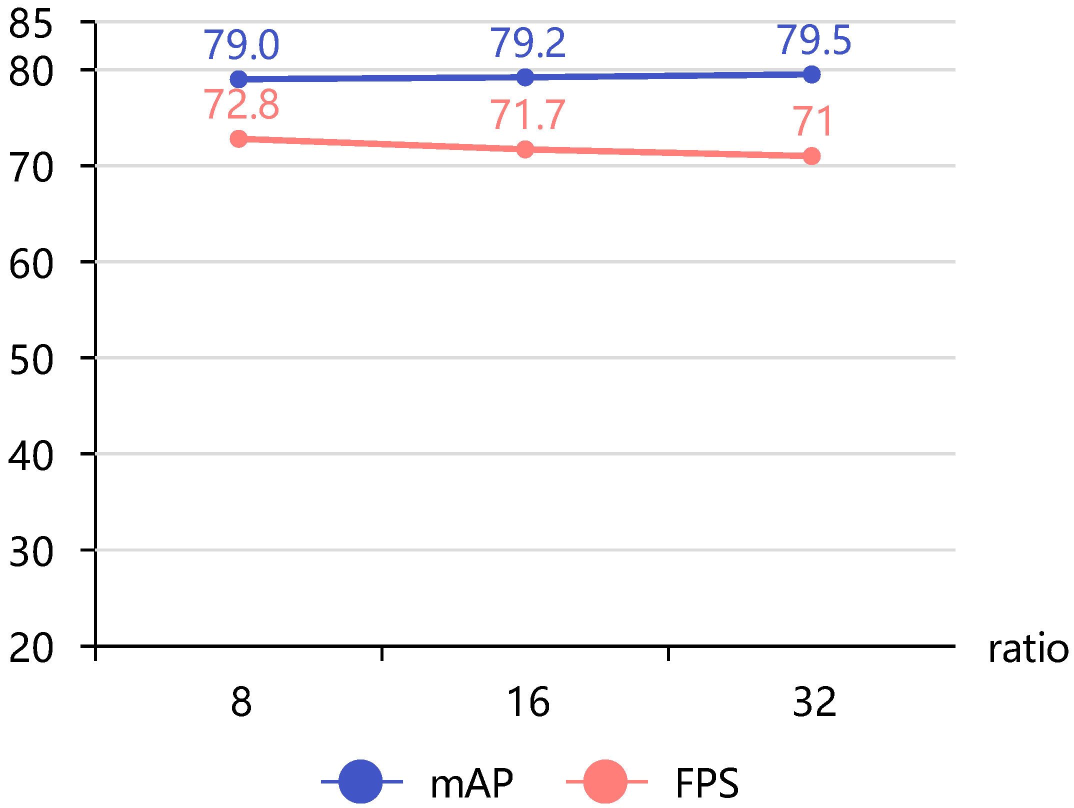
In the channel refinement part of the FRM, we had to feed the channel weights obtained from pooling into $Con{v}_1$ to compress the number of channels and then reduced them in $Con{v}_2$. The choice of compression ratio thus affected the detection performance. Figure 11 shows a plot of accuracy over compression ratio. The detection accuracy gradually increased but the detection speed decreased. Therefore, a different ratio can be chosen according to the actual production needs. To balance accuracy and speed, a final ratio of 32 was chosen here, which was compressed to 1/32 of the original.

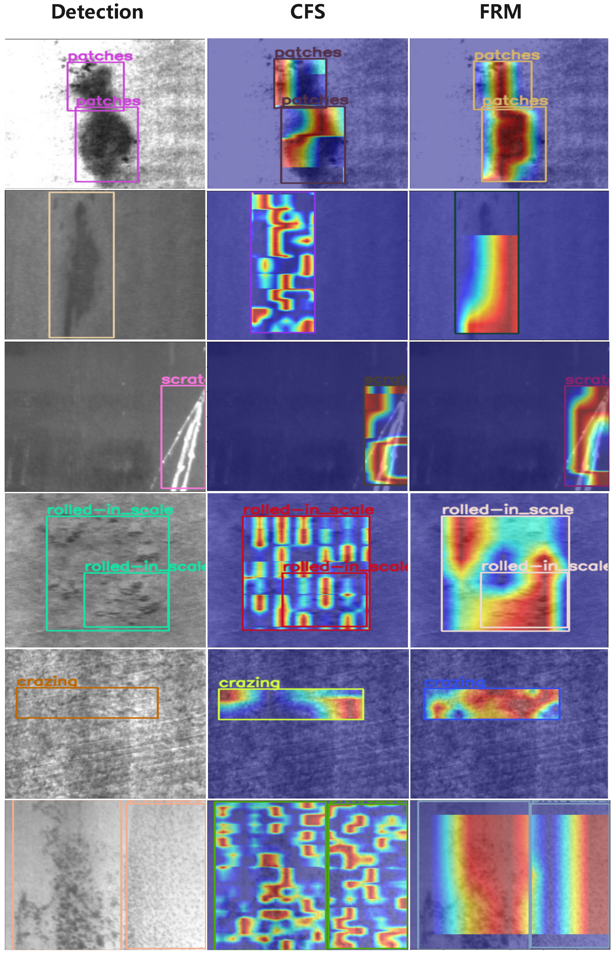
As shown in Figure 12, we extracted the same layers in the CFS and FRM to generate the feature class activation map Eigen-CAM [39] and visualize the features learned by both. We can see that the features learned by CFS were more scattered, due to the semantic conflict and redundancy brought by the fusion of different scale feature maps and the features learned by the FRM being more focused after filtering and guiding, which also proved the effectiveness of our FRM.

Our model only adds the FRM in layers $P_0$∼$P_3$ (as shown in Figure 2), while the FRM is not applied in layers $P_4$ and $P_5$, since the feature maps of these two layers are small ($3\times 3$ and $1\times 1$, respectively) and they do not have much conflict and redundant information by themselves. If the FRM was added in this case, then it would reduce the detection performance. As shown in

Table 9. Results of adding FRM in order from $P_0$ to $P_5$ layers.

Layer	Ratio	mAP	FPS
$P_0$∼$P_3$	8	79.0	72.8
$P_0$∼$P_4$	8	78.7	70
$P_0$∼$P_5$	8	78.8	67
$P_0$∼$P_3$	16	79.2	71.7
$P_0$∼$P_4$	16	78.7	69
$P_0$∼$P_5$	16	78.9	67
$P_0$∼$P_3$	32	79.5	71.3
$P_0$∼$P_4$	32	78.8	68
$P_0$∼$P_5$	32	78.3	65

, we added the FRM to $P_4$ and $P_5$ layers after adding the FRM to $P_0$∼$P_3$ but the results became worse.

5. Discussion

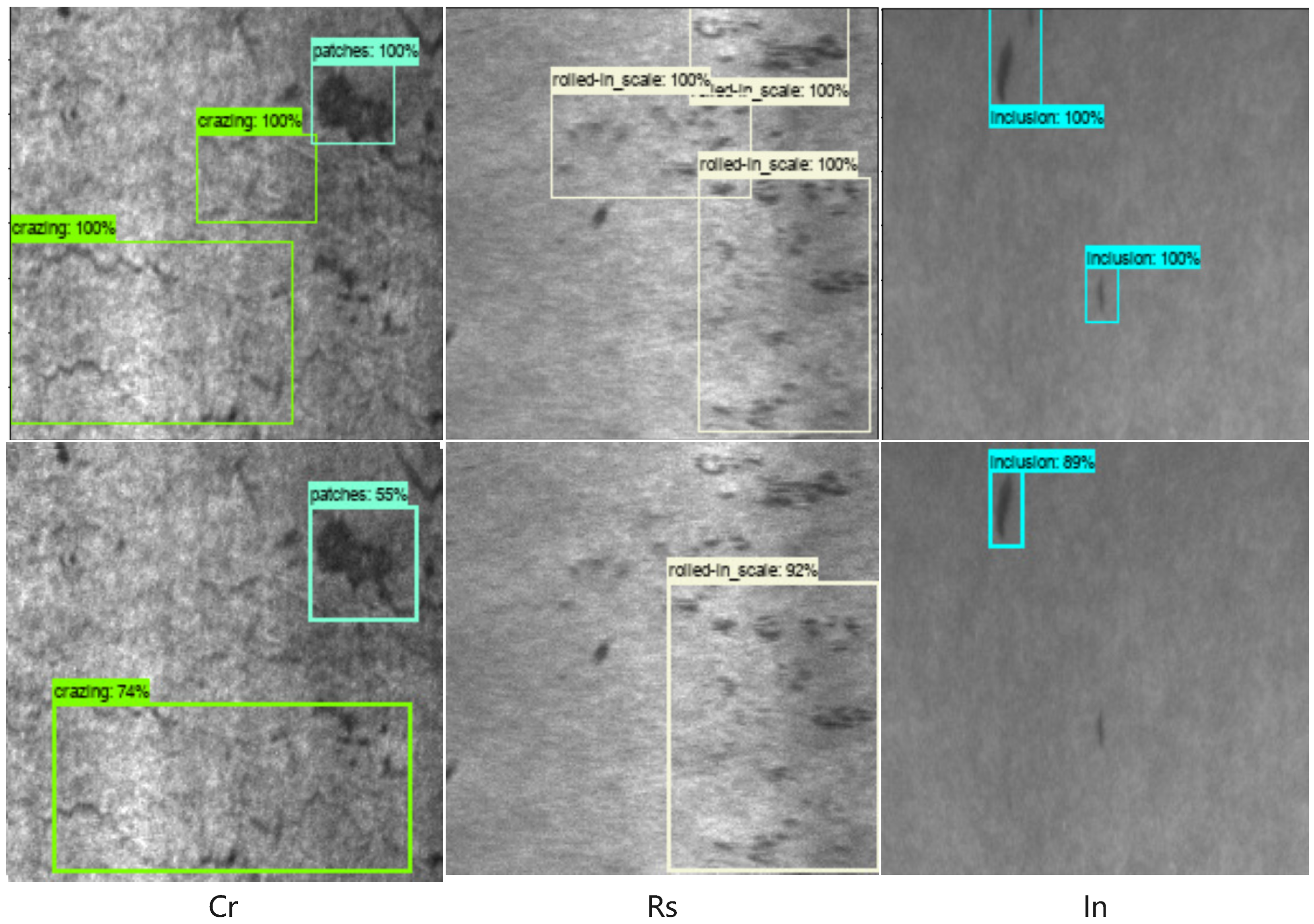
While our model achieved a very good average performance on NEU-DET, there were still a few cases of detection failure. In Table 5, the accuracy of Cr and Rs was the lowest, followed by In. In particular, the accuracy of Cr was only 47%. Therefore, the model had different degrees of detection errors in these categories, as shown in Figure 13. The main reason for this was that with a low resolution and low contrast, the objects are smaller and widely scattered, which is difficult for anchor-based models to detect. In particular, the shape of crazing is very thin and widely distributed, which caused great difficulties for the target positioning of the model.

Some possible methods we can develop to improve the performance include the following: First, expand the data set, to enable the model to learn more information. Second, use anchor-free techniques for detection. Third, combine a transformer model to extract global features, which would help the model to better locate target defects.

6. Conclusions

Steel defects with small interclass and large intraclass differences and the high requirement for detection speed in industrial production raise significant challenges regarding their detection. These are the two main problems that hinder the development of strip steel surface defect detection. In order to solve these issues, this study proposed a new detection method, which is a lightweight model with high detection accuracy and speed. We followed the classic frame of the SSD. We design a CFS in the encoding stage, which introduced more contextual information for the multiscale feature map and improved the detection accuracy, while maintaing the speed. In the decoding stage, a FRM was used after the predicted feature map, in order to filter out the semantic conflicts and redundancies brought by the feature map fusion of different scales. This further improved the detection accuracy. Our experiments validated our method. In particular, our experiments showed that our method achieved a comparatively better performance than the other methods, in terms of both accuracy and efficiency.

References

- Liu, W.; Anguelov, D.; Erhan, D.; Szegedy, C.; Reed, S.; Fu, C.Y.; Berg, A.C. SSD: Single Shot MultiBox Detector. In Proceedings of the Computer Visio (ECCV 2016), Amsterdam, The Netherlands, 11–14 October 2016; Leibe, B., Matas, J., Sebe, N., Welling, M., Eds.; Springer International Publishing: Cham, Switzerland, 2016; pp. 21–37. [Google Scholar] [CrossRef]
- He, K.; Zhang, X.; Ren, S.; Sun, J. Deep Residual Learning for Image Recognition. In Proceedings of the IEEE Conference on Computer Vision and Pattern Recognition (CVPR), Las Vegas, NV, USA, 27–30 June 2016. [Google Scholar] [CrossRef]
- Song, K.; Yan, Y. A noise robust method based on completed local binary patterns for hot-rolled steel strip surface defects. Appl. Surf. Sci. 2013, 285, 858–864. [Google Scholar] [CrossRef]
- Fu, C.Y.; Liu, W.; Ranga, A.; Tyagi, A.; Berg, A.C. Dssd: Deconvolutional single shot detector. arXiv 2017, arXiv:1701.06659. [Google Scholar] [CrossRef]
- Jeong, J.; Park, H.; Kwak, N. Enhancement of SSD by concatenating feature maps for object detection. arXiv 2017, arXiv:1705.09587. [Google Scholar] [CrossRef]
- Woo, S.; Park, J.; Lee, J.Y.; Kweon, I.S. CBAM: Convolutional Block Attention Module. In Proceedings of the European Conference on Computer Vision (ECCV), Munich, Germany, 8–14 September 2018. [Google Scholar] [CrossRef]
- Wang, Q.; Wu, B.; Zhu, P.; Li, P.; Zuo, W.; Hu, Q. Supplementary material for ‘ECA-Net: Efficient channel attention for deep convolutional neural networks. In Proceedings of the 2020 IEEE/CVF Conference on Computer Vision and Pattern Recognition, Seattle, WA, USA, 14–19 June 2020; IEEE: Seattle, WA, USA, 2020; pp. 13–19. [Google Scholar] [CrossRef]
- Di, H.; Ke, X.; Peng, Z.; Dongdong, Z. Surface defect classification of steels with a new semi-supervised learning method. Opt. Lasers Eng. 2019, 117, 40–48. [Google Scholar] [CrossRef]
- Li, Z.; Wu, C.; Han, Q.; Hou, M.; Chen, G.; Weng, T. CASI-Net: A Novel and Effect Steel Surface Defect Classification Method Based on Coordinate Attention and Self-Interaction Mechanism. Mathematics 2022, 10, 963. [Google Scholar] [CrossRef]
- Fu, G.; Sun, P.; Zhu, W.; Yang, J.; Cao, Y.; Yang, M.Y.; Cao, Y. A deep-learning-based approach for fast and robust steel surface defects classification. Opt. Lasers Eng. 2019, 121, 397–405. [Google Scholar] [CrossRef]
- Tang, l.B.; Kong, J.; Wu, S. Review of surface defect detection based on machine vision. J. Image Graph. 2017, 22, 1640–1663. [Google Scholar]
- Luo, Q.; Sun, Y.; Li, P.; Simpson, O.; Tian, L.; He, Y. Generalized completed local binary patterns for time-efficient steel surface defect classification. IEEE Trans. Instrum. Meas. 2018, 68, 667–679. [Google Scholar] [CrossRef]
- Liu, K.; Wang, H.; Chen, H.; Qu, E.; Tian, Y.; Sun, H. Steel surface defect detection using a new Haar–Weibull-variance model in unsupervised manner. IEEE Trans. Instrum. Meas. 2017, 66, 2585–2596. [Google Scholar] [CrossRef]
- Mei, S.; Yang, H.; Yin, Z. An unsupervised-learning-based approach for automated defect inspection on textured surfaces. IEEE Trans. Instrum. Meas. 2018, 67, 1266–1277. [Google Scholar] [CrossRef]
- Luo, Q.; Fang, X.; Sun, Y.; Liu, L.; Ai, J.; Yang, C.; Simpson, O. Surface defect classification for hot-rolled steel strips by selectively dominant local binary patterns. IEEE Access 2019, 7, 23488–23499. [Google Scholar] [CrossRef]
- Li, H.; Fu, X.; Huang, T. Research on surface defect detection of solar pv panels based on pre-training network and feature fusion. In Proceedings of the IOP Conference Series: Earth and Environmental Science; IOP Publishing: Bristol, UK, 2021; Volume 651, p. 022071. [Google Scholar] [CrossRef]
- Girshick, R.; Donahue, J.; Darrell, T.; Malik, J. Rich feature hierarchies for accurate object detection and semantic segmentation. In Proceedings of the IEEE Conference on Computer Vision and Pattern Recognition, Columbus, OH, USA, 23–28 June 2014; pp. 580–587. [Google Scholar] [CrossRef]
- Girshick, R. Fast r-cnn. In Proceedings of the IEEE International Conference on Computer Vision, Santiago, Chile, 7–13 December 2015; pp. 1440–1448. [Google Scholar] [CrossRef]
- Ren, S.; He, K.; Girshick, R.; Sun, J. Faster r-cnn: Towards real-time object detection with region proposal networks. IEEE Trans. Pattern Anal. Mach. Intell. 2017, 39, 1137–1149. [Google Scholar] [CrossRef] [PubMed]
- Lin, T.Y.; Goyal, P.; Girshick, R.; He, K.; Dollár, P. Focal loss for dense object detection. In Proceedings of the IEEE International Conference on Computer Vision, Venice, Italy, 22–29 October 2017; pp. 2980–2988. [Google Scholar] [CrossRef]
- Redmon, J.; Farhadi, A. Yolov3: An incremental improvement. arXiv 2018, arXiv:1804.02767. [Google Scholar] [CrossRef]
- Bochkovskiy, A.; Wang, C.Y.; Liao, H.Y.M. Yolov4: Optimal speed and accuracy of object detection. arXiv 2020, arXiv:2004.10934. [Google Scholar] [CrossRef]
- Jocher, G.; Stoken, A.; Borovec, J.; Chaurasia, A.; Changyu, L.; Laughing, A.; Hogan, A.; Hajek, J.; Diaconu, L.; Marc, Y.; et al. ultralytics/yolov5: v5. 0-YOLOv5-P6 1280 models AWS Supervise. ly and YouTube integrations. Zenodo 2021, 11, 4679653. [Google Scholar]
- Ge, Z.; Liu, S.; Wang, F.; Li, Z.; Sun, J. Yolox: Exceeding yolo series in 2021. arXiv 2021, arXiv:2107.08430. [Google Scholar] [CrossRef]
- Zhao, W.; Chen, F.; Huang, H.; Li, D.; Cheng, W. A new steel defect detection algorithm based on deep learning. Comput. Intell. Neurosci. 2021, 2021, 5592878. [Google Scholar] [CrossRef] [PubMed]
- Hatab, M.; Malekmohamadi, H.; Amira, A. Surface defect detection using YOLO network. In Proceedings of the SAI Intelligent Systems Conference, London, UK, 3–4 September 2020; pp. 505–515. [Google Scholar] [CrossRef]
- Kou, X.; Liu, S.; Cheng, K.; Qian, Y. Development of a YOLO-V3-based model for detecting defects on steel strip surface. Measurement 2021, 182, 109454. [Google Scholar] [CrossRef]
- He, Y.; Song, K.; Meng, Q.; Yan, Y. An end-to-end steel surface defect detection approach via fusing multiple hierarchical features. IEEE Trans. Instrum. Meas. 2019, 69, 1493–1504. [Google Scholar] [CrossRef]
- Cheng, X.; Yu, J. RetinaNet with difference channel attention and adaptively spatial feature fusion for steel surface defect detection. IEEE Trans. Instrum. Meas. 2020, 70, 1–11. [Google Scholar] [CrossRef]
- Simonyan, K.; Zisserman, A. Very deep convolutional networks for large-scale image recognition. arXiv 2014, arXiv:1409.1556. [Google Scholar] [CrossRef]
- Lin, T.Y.; Dollár, P.; Girshick, R.; He, K.; Hariharan, B.; Belongie, S. Feature pyramid networks for object detection. In Proceedings of the IEEE Conference on Computer Vision and Pattern Recognition, Honolulu, HI, USA, 21–26 July 2017; pp. 2117–2125. [Google Scholar] [CrossRef]
- Long, J.; Shelhamer, E.; Darrell, T. Fully convolutional networks for semantic segmentation. In Proceedings of the IEEE Conference on Computer Vision and Pattern Recognition, Boston, MA, USA, 7–12 June 2015; pp. 3431–3440. [Google Scholar] [CrossRef]
- Noh, H.; Hong, S.; Han, B. Learning deconvolution network for semantic segmentation. In Proceedings of the IEEE International Conference on Computer Vision, Santiago, Chile, 11–18 December 2015; pp. 1520–1528. [Google Scholar] [CrossRef]
- Zeiler, M.D.; Fergus, R. Visualizing and understanding convolutional networks. In Proceedings of the European Conference on Computer Vision, Zurich, Switzerland, 6–12 September 2014; pp. 818–833. [Google Scholar] [CrossRef]
- Russakovsky, O.; Deng, J.; Su, H.; Krause, J.; Satheesh, S.; Ma, S.; Huang, Z.; Karpathy, A.; Khosla, A.; Bernstein, M.; et al. Imagenet large scale visual recognition challenge. Int. J. Comput. Vis. 2015, 115, 211–252. [Google Scholar] [CrossRef]
- Xie, S.; Girshick, R.; Dollár, P.; Tu, Z.; He, K. Aggregated residual transformations for deep neural networks. In Proceedings of the IEEE Conference on Computer Vision and Pattern Recognition, Honolulu, HI, USA, 21–26 July 2017; pp. 1492–1500. [Google Scholar] [CrossRef]
- Li, J.; Su, Z.; Geng, J.; Yin, Y. Real-time detection of steel strip surface defects based on improved yolo detection network. IFAC-PapersOnLine 2018, 51, 76–81. [Google Scholar] [CrossRef]
- Jocher, G.; Chaurasia, A.; Qiu, J. YOLO by Ultralytics, 2023. Available online: https://doi.org/10.5281/zenodo.7347926 (accessed on 17 May 2023).
- Muhammad, M.B.; Yeasin, M. Eigen-cam: Class activation map using principal components. In Proceedings of the 2020 International Joint Conference on Neural Networks (IJCNN), Glasgow, UK, 19–24 July 2020; pp. 1–7. [Google Scholar] [CrossRef]
Figure 1.
Samples of targets: (a–c) are sample Classic dataset. (d–f) are sample steel surface defects.
Figure 2.
Model structure.
Figure 3.
Context fusion structure.
Figure 4.
Feature refinement module.
Figure 5.
Channel refinement.
Figure 6.
Spatial refinement.
Figure 7.
NEU-DET dataset.
Figure 8.
Model detection performance.
Figure 9.
Three types of feature map fusion in CFS.
Figure 10.
Detection accuracy of multiscale targets.
Figure 11.
Different compression ratios.
Figure 12.
Comparison of the effects of the class activation map of FRM and CFS.
Figure 13.
Examples of failed detection with our model on NEU-DET, where the first line is the ground truth. Cr: crazing, Rs: rolled-in scale, In: inclusion.