Research on High-Quality Control Technology for Three-Phase PWM Rectifier

Abstract

With the development of power-electronics technology, PWM rectifiers are widely used in many fields. They are especially suitable for high-precision- and high-efficiency-application scenarios, such as communication and industrial control. Although it has many advantages, overshoot control during startup is a challenge. Therefore, this paper first derives the input–output mathematical model through equation establishment and dq-coordinate transformation. Next, a voltage and current double closed-loop simulation model is established in MATLAB/Simulink, and its control effect is analyzed. On this basis, a new voltage-setting strategy is designed to reduce the output-voltage overshoot of the PWM rectifier when starting. The simulation results demonstrate that the strategy has a good application effect and can contain starting-voltage overshooting from 12.88% to 0.925%. Moreover, the principle of this strategy is simpler and easier to understand and implement compared with traditional strategies.

1. Introduction

Rectification, as an indispensable part of the field of power electronics, is undoubtedly of great importance. With the development of technology, the types of rectifier are increasing in number. According to the basic circuit structures they use, they can be roughly divided into single-phase half-wave rectification, single-phase whole-wave rectification, three-phase half-wave rectification, and three-phase whole-wave rectification.

In particular, the advantages of single-phase half-wave rectifiers comprise simplicity and low cost, whereas their output ripple is relatively large [1]. Although single-phase whole-wave rectifiers have a small output ripple and high efficiency, they require two diodes for rectification [2]. The advantage of three-phase half-wave rectifiers is that the output voltage is relatively stable, while it requires more diodes and capacitors [3]. Finally, the output voltage of three-phase whole-wave rectifiers is stable and efficient, with the only drawback being the need for more components.

Different types of rectifier are applicable in different scenarios. Considering the multiple factors above, the use of three-phase whole-wave rectification circuits is common. In particular, PWM (pulse-width modulation) rectifiers have the advantages of good sinusoidal input current, low harmonic content, and a high power factor [4,5]. These PWM rectifiers use an amplifier element to provide amplification and regulation while rectifying. Although passive rectifiers that make it possible to reach low THD already exist [6,7], PWM rectifiers offer the advantages of stable output voltage and output waveforms with high accuracy, while passive rectifiers cannot provide these functions. With the increasingly strict working standards of electrical equipment, the range of use of PWM rectifiers is becoming increasingly widespread, including the following situations:

• Power converters: The PWM rectifiers can convert AC/DC power into DC of various voltages in the application of power conversion [8,9].
• Motor controllers: A PWM rectifier can be used to control the speed and output power of the motor, as well as the forward and reverse rotation of the motor [10,11,12,13].
• Energy-feedback systems: in applications such as new-energy vehicles and wind turbines, PWM rectifiers can feed energy back to the power grid [14,15,16].
• Chargers: a PWM rectifier can control the current within a certain range to achieve safe and fast charging and control the output voltage of the charger through the PWM duty cycle [17,18].

A three-phase PWM rectifier is an electronic circuit that is adopted to convert three-phase alternating currents into direct currents with pulse-width modulation. Its working principle is to achieve current control and conversion by controlling the conduction and cutoff of three groups of switch tubes in a three-phase bridge rectifier. The PWM controller adjusts the conduction time of each switch tube based on the amplitude and phase of the input signal. The longer the conduction time of the switch tube, the higher the output voltage, and vice versa. When the conduction time is adjusted, its average voltage value throughout the entire cycle reaches the setting value. After it is filtered by a capacity, the output is a smooth DC.

The open-loop control of the three-phase PWM rectifier controls the output voltage of the rectifier by modulating the three-phase power supply with the PWM. Open-loop control indicates that there is no feedback loop with which to adjust the PWM signal, and the control signal is fixed. In other words, open-loop control is not accurate. Thus, direct-current control methods and double closed-loop control structures are generally used in the dq rotating coordinate system in the control of PWM rectifiers. In this control strategy, the controller immediately detects the change through the feedback loop and adjusts it when the output voltage changes, allowing the DC side to track back to the given value in a short period of time. This control method can improve the stability and accuracy of PWM rectifiers, making it suitable for application scenarios with high precision and good stability requirements for output voltage [19].

The outer voltage loop is utilized to control the output voltage of the rectifier, and the inner current loop realizes the waveform and phase control of the grid-side current [19]. The control signal is modulated into a trigger signal after reverse transformation. The overall model construction is illustrated in Figure 1.

The system designed in [20] has high efficiency in tracking the maximum power point and has a low THD value, demonstrating the significant potential of PWM rectifiers in the field of renewable energy. The single-phase open-line fault of a three-phase PWM rectifier was theoretically analyzed and a corresponding diagnosis scheme was proposed so as to improve improves the stability and reliability of the three-phase PWM rectifier [21]. A capacitive energy-storage feedback-control strategy with a current inner loop and DC-side capacitive energy storage as the outer loop was presented [22] to overcome slow output-voltage regulation when the load changes and to improve the dynamic characteristics of the system. Similarly, a different control strategy with voltage squared as the outer loop and model-predicted current as the inner loop was designed to address the same problem [23]. The results of the latter study reinforced the fast-tracking ability of the system to DC output voltage. The impact current at the start-up of the rectifier was lowered [24], although, in that study, the output-voltage overshoot was neglected.

In this paper, the coordinate-transformation process from an abc three-phase static coordinate system is introduced to a dq rotating coordinate system. Furthermore, the input–output mathematical model of the PWM rectifier is deduced. Next, the widely used double-closed-loop control system of voltage and current is simulated and validated, and a new stepped voltage-setting strategy is designed to tackle the problem of excessive startup-voltage overshoot. Instead of inputting the full voltage as the given voltage directly, the given voltage value is inputted in the form of step increase. The simulation results reveal that the problem of excessive voltage overshoot is significantly relieved with this new strategy. Compared with traditional methods, such as fuzzy-algorithm control and voltage-square-loop control, the control effect of this strategy is slightly better, and the design of its control system is much simpler.

This article is organized as follows. In Section 2, the input–output mathematical model of the PWM rectifier is established, and the controller-design scheme is provided. In Section 3, the simulation results are analyzed, and an optimization plan is proposed to deal with the excessive overshoot of the starting voltage on the DC side. Finally, the conclusions are drawn in Section 4. In addition, for the convenience of readers’ understanding, the abbreviations in this article can be found in the Abbreviations.

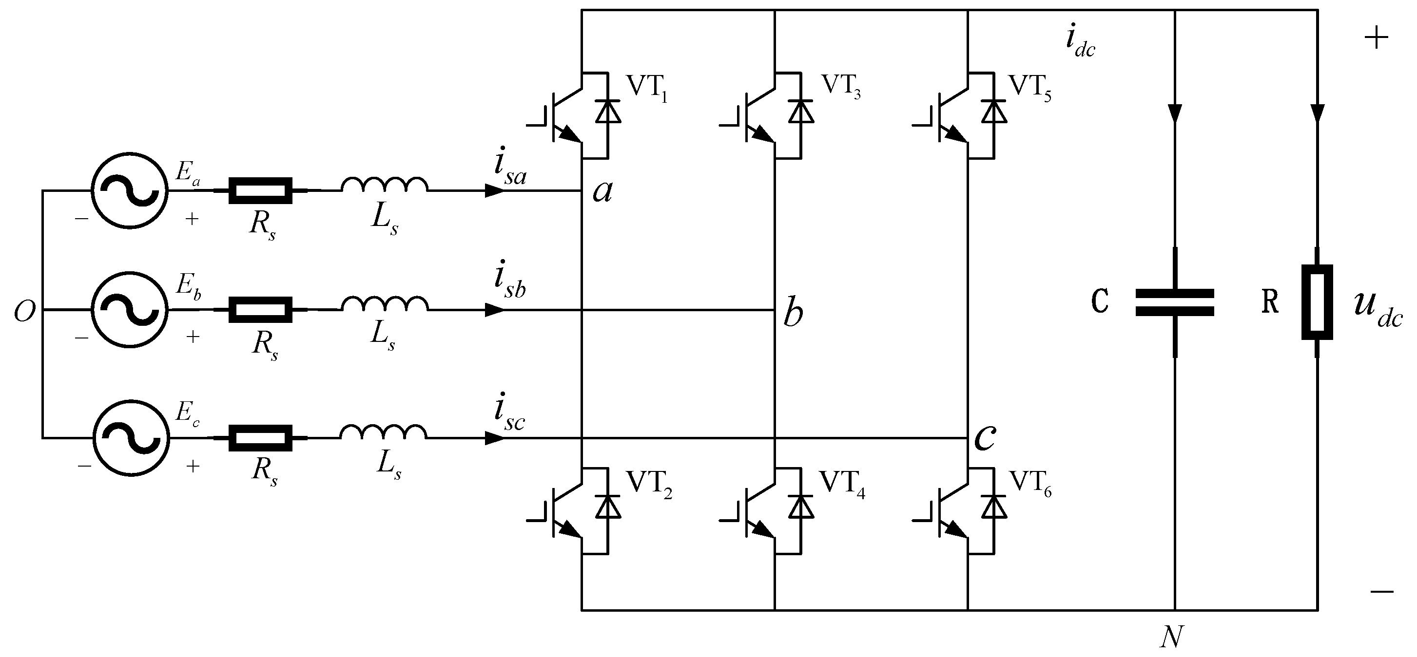
2. Mathematical Modeling of Three-Phase VSR

The main circuit of the three-phase PWM rectifier circuit is depicted in Figure 2, where $E_a,E_b,E_c$ represent the power-supply voltage of each phase grid-side, $i_{sa},i_{sb},i_{sc}$ denote the input current of each phase grid-side, $L_s$ indicates the filter inductance, $R_s$ signifies the sum of the filter-inductance equivalent resistance and the switching-tube-loss equivalent resistance, C represents the DC-side capacitor, $u_{dc}$ is the DC-side output voltage, $i_{dc}$ is the DC-side output current, R stands for the load resistance, and ${\mathrm{VT}}_{1-6}$ denotes the IGBT with freewheeling diodes.

The input–output mathematical model of the three-phase PWM rectifier should be derived to understand its operating principle and facilitate its control. First, KVL and KCL equations are written for the circuit list to obtain:

$$\{\begin{array}{l}-E_a+R_s{i}_{sa}+L_s\frac{d{i}_{sa}}{dt}+u_{ao}=0\\ -E_b+R_s{i}_{sb}+L_s\frac{d{i}_{sb}}{dt}+u_{bo}=0\\ -E_c+R_s{i}_{sc}+L_s\frac{d{i}_{sc}}{dt}+u_{co}=0\\ C\frac{d{u}_{dc}}{dt}+\frac{u_{dc}}{R}=i_{dc}\end{array}$$

(1)

If the switching value $S_j(j=a,b,c)$ is used to replace $u_{jo}(j=a,b,c)$ in the formula ($S_j=1$ represents upper bridge arm conduction in j phase; $S_j=0$ indicates lower bridge arm conduction), the following conclusions can be drawn regarding the characteristics of a three-phase power supply $E_a+E_b+E_c=0$.

$$\{\begin{array}{l}{L}_s\frac{d{i}_{sa}}{dt}=E_a-R_s{i}_{sa}-\left[S_a-\frac{1}{3}(S_a+S_b+S_c)\right]U_{dc}\\ L_s\frac{d{i}_{sb}}{dt}=E_b-R_s{i}_{sb}-\left[S_b-\frac{1}{3}(S_a+S_b+S_c)\right]U_{dc}\\ L_s\frac{d{i}_{sc}}{dt}=E_c-R_s{i}_{sc}-\left[S_c-\frac{1}{3}(S_a+S_b+S_c)\right]U_{dc}\\ C\frac{d{u}_{dc}}{dt}=i_a{S}_a+i_a{S}_a+i_a{S}_a-\frac{u_{dc}}{R}\end{array}$$

(2)

This is the mathematical model of a PWM rectifier in a three-phase stationary coordinate system. However, the equation system has four equations, making it excessively complex to design a control system. Therefore, mathematical simplification is still needed. Next, the transformation of the abc three-phase stationary-coordinate system is introduced to the dq rotating-coordinate system.

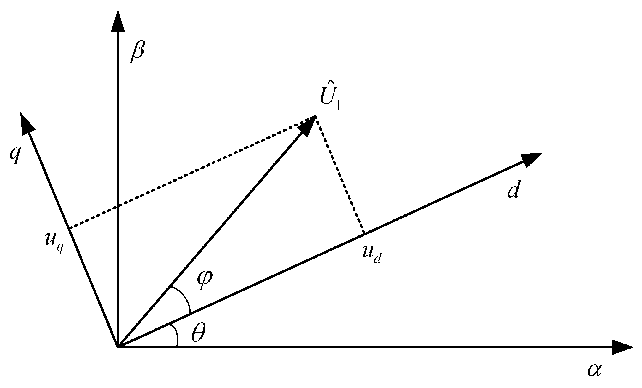
2.1. Coordinate Transformation and Establishment of the dq Model

For the general mathematical model of a three-phase PWM rectifier, the control is more difficult, since the variables on the AC side are time-varying, though the physical significance is clear. On this basis, a solution is proposed. Specifically, the transformation is coordinated into a synchronous rotation-coordinate system (d,q) to achieve simplified control requirements [25]. The process of the transformation is described below.

Before the introduction of the concrete transformation process, the basic concept and some formulas of coordinate transformation should be introduced first.

2.1.1. Three-Phase Stationary Coordinate System to Two-Phase Stationary Coordinate System

The three-phase voltage or current can be adopted to synthesize a space-vector equivalent, called a universal vector or composite vector. Concerning the convenience of expression, the moment $u_b=0$ is taken. Thus, the relationships between $u_a,u_b,u_c$ and $U$ are illustrated in Figure 3.

Since the resulting voltage vector is a rotation vector, it is difficult to describe it in the three-phase static coordinate system. Therefore, the introduction of the $\alpha$-$\beta$ coordinate system (two static coordinate systems) is necessary. Figure 3 presents its relation to the original coordinate system.

As shown in the figure, the space vectors d and e in the two-phase static coordinate system and the original vectors $u_a$ and $u_c$ can synthesize the same rotation vector, in order to complete the transformation from the three-phase static coordinate system to the two-phase static coordinate system. Nonetheless, coefficient 2/3 is introduced into the transformation, since the amplitude of d and e is 3/2 times that of $u_a$ and $u_c$. When there is an unbalanced component in the three-phase voltage:

$$u_0=\frac{1}{3}\left(u_a+u_b+u_c\right)$$

(3)

Two matrices are set as:

$$U_{\beta \alpha 0}={\left(\begin{array}{ccc}{u}_{\beta }& u_{\alpha }& u_0\end{array}\right)}^{\tau },U_{abc}={\left(\begin{array}{ccc}{u}_a& u_b& u_c\end{array}\right)}^{\tau }$$

Next, a matrix $M$ is set to satisfy:

$$U_{\beta \alpha 0}=M{U}_{abc}$$

(4)

The transformation matrix $M$ and its inverse matrix $M^{-1}$ are expressed as:

$$M=\frac{2}{3}\left(\begin{array}{ccc}1& -\frac{1}{2}& -\frac{1}{2}\\ 0& -\frac{\sqrt{3}}{2}& \frac{\sqrt{3}}{2}\\ \frac{1}{2}& \frac{1}{2}& \frac{1}{2}\end{array}\right)M^{-1}=\left(\begin{array}{ccc}1& 0& 1\\ -\frac{1}{2}& -\frac{\sqrt{3}}{2}& 1\\ -\frac{1}{2}& \frac{\sqrt{3}}{2}& 1\end{array}\right)$$

(5)

2.1.2. Two-Phase Stationary Coordinate System to Two-Phase Rotation Coordinate System

Although the two-phase stationary coordinate system can describe the resultant voltage vector, it cannot achieve the goal of transforming into the time-invariant. Hence, a new rotating coordinate system is introduced, and it is regarded as a fixed value if it is rotated synchronously with the synthesized voltage.

The two-phase rotating coordinate system is divided into a d-axis and a q-axis. The d-axis is orthogonal to the q-axis, and the rotational angular velocity is the three-phase voltage angular frequency $\omega$. As demonstrated in Figure 4, the initial position of the d-axis is the same as that of the $\alpha$-axis in the two-phase stationary coordinate system; the q-axis advances the d-axis by $90$°. The angle $\theta$ between the d-axis and the $\alpha$-axis can be used to characterize the current position of the dq coordinate axis. The angle of rotation is satisfied:

$$\theta =\omega t$$

(6)

Next, its voltage vector is decomposed into the d-axis and the q-axis to obtain:

$$\{\begin{array}{l}{u}_{\alpha }=u_d\cos \theta +u_q\cos \left(\frac{\pi }{2}+\theta \right)\\ u_{\beta }=u_d\cos \left(\frac{\pi }{2}-\theta \right)+u_q\cos \theta \end{array}$$

(7)

It is written in a matrix form, as follows:

$$\left(\begin{array}{c}{u}_{\alpha }\\ u_{\beta }\end{array}\right)=\left(\begin{array}{cc}\cos \theta & \sin \theta \\ -\sin \theta & \cos \theta \end{array}\right)\left(\begin{array}{c}{u}_d\\ u_q\end{array}\right)$$

(8)

2.1.3. Three-Phase Stationary Coordinate System to Two-Phase Rotation Coordinate System

In the case of the unbalanced component $u_0$, the three-phase voltage is converted twice to obtain Equation (9) based on the results of Section 2.1.1 and Section 2.1.2.

$$\left(\begin{array}{c}{u}_d\\ u_q\end{array}\right)=\frac{2}{3}\left(\begin{array}{ccc}\cos \theta & \cos \left(\theta -\frac{2\pi }{3}\right)& \cos \left(\theta +\frac{2\pi }{3}\right)\\ -\sin \theta & -\sin \left(\theta -\frac{2\pi }{3}\right)& -\sin \left(\theta +\frac{2\pi }{3}\right)\end{array}\right)\left(\begin{array}{c}{u}_a\\ u_b\\ u_c\end{array}\right)$$

(9)

The coefficient matrix is added to the widely reversible matrix:

$$u_0=\frac{1}{3}\left(u_a+u_b+u_c\right)$$

(10)

$$\left(\begin{array}{c}{u}_d\\ u_q\\ u_0\end{array}\right)=\frac{2}{3}\left(\begin{array}{ccc}\cos \theta & \cos \left(\theta -\frac{2\pi }{3}\right)& \cos \left(\theta +\frac{2\pi }{3}\right)\\ -\sin \theta & -\sin \left(\theta -\frac{2\pi }{3}\right)& -\sin \left(\theta +\frac{2\pi }{3}\right)\\ \frac{1}{2}& \frac{1}{2}& \frac{1}{2}\end{array}\right)\left(\begin{array}{c}{u}_a\\ u_b\\ u_c\end{array}\right)$$

(11)

Inverting Equation (11) yields:

$$\left(\begin{array}{c}{u}_a\\ u_b\\ u_c\end{array}\right)=\frac{2}{3}\left(\begin{array}{ccc}\cos \theta & -\sin \theta & 1\\ \cos \left(\theta -\frac{2\pi }{3}\right)& -\sin \left(\theta -\frac{2\pi }{3}\right)& 1\\ \cos \left(\theta +\frac{2\pi }{3}\right)& -\sin \left(\theta +\frac{2\pi }{3}\right)& 1\end{array}\right)\left(\begin{array}{c}{u}_d\\ u_q\\ u_0\end{array}\right)$$

(12)

2.1.4. dq Model of Three-Phase VSR

The switching-function model of three-phase VSR [25] is:

$$\{\begin{array}{l}C\frac{d{u}_{dc}}{dt}={\displaystyle \sum _{k=a,b,c}{i}_k{s}_k-i_L}\\ L\frac{d{i}_k}{dt}+R_s{i}_k=e_k-u_{dc}\left(s_k-\frac{1}{3}{\displaystyle \sum _{j=a,b,c}{X}_j}\right)\\ {\displaystyle \sum _{k=a,b,c}{e}_k}={\displaystyle \sum _{k=a,b,c}{i}_k}=0\end{array}$$

(13)

where $s_k$ denotes the logic switching function, and $i_L$ represents the DC-side load current. Based on the discussion in Section 2.1.1, there are:

$$\left(\begin{array}{c}{x}_a\\ x_b\\ x_c\end{array}\right)=\frac{2}{3}\left(\begin{array}{cc}1& 0\\ -\frac{1}{2}& -\frac{\sqrt{3}}{2}\\ -\frac{1}{2}& \frac{\sqrt{3}}{2}\end{array}\right)\left(\begin{array}{c}{x}_{\alpha }\\ x_{\beta }\end{array}\right)$$

(14)

Substituting Equation (14) into Equation (13) yields:

$$\{\begin{array}{l}C\frac{d{u}_{dc}}{dt}=\frac{3}{2}\left(i_{\beta }{s}_{\beta }+i_{\alpha }{s}_{\alpha }-i_L\right)\\ L_s\frac{d{i}_{\beta }}{dt}+R_s{i}_{\beta }=e_{\beta }-u_{dc}{s}_{\beta }\\ L_s\frac{d{i}_{\alpha }}{dt}+R_s{i}_{\alpha }=e_{\alpha }-u_{dc}{s}_{\alpha }\end{array}$$

(15)

where $s_{\alpha }$ and $s_{\beta }$ indicate the logical switching functions in the $\alpha$-$\beta$ coordinate system.

The complex vector $X_{\alpha \beta }$ is constructed to satisfy:

$$X_{\alpha \beta }=x_{\beta }-j{x}_{\alpha }$$

$$X_{\alpha \beta }\in \{E_{\alpha \beta },I_{\alpha \beta },S_{\alpha \beta }\}$$

The complex vector form of Equation (15) is:

$$\{\begin{array}{l}C\frac{d{u}_{dc}}{dt}=\frac{3}{2}\mathrm{Re}\{I_{\alpha \beta }{\overline{S}}_{\alpha \beta }\}-i_L\\ L_s\frac{d{I}_{\alpha \beta }}{dt}+R_s{I}_{\alpha \beta }=E_{\alpha \beta }-u_{dc}{S}_{\alpha \beta }\end{array}$$

(16)

where ${\overline{S}}_{\alpha \beta }$ signifies a conjugate vector.

After introducing rotation factor ${\mathrm{e}}^{\mathrm{j}\theta }$, the synthetic complex vector can be expressed as:

$$\{\begin{array}{l}{e}^{j\theta }{X}_{dq}=X_{\alpha \beta }\\ \theta ={\displaystyle \int \omega dt}\\ \omega =2\pi f\end{array}$$

(17)

Thus, the complex vector equation is obtained, as follows:

$$\{\begin{array}{l}C\frac{dy}{dx}=\frac{3}{2}\mathrm{Re}\{I_{dq}{\overline{S}}_{dq}\}-i_L\\ L_s\frac{d{I}_{dq}}{dt}+j\omega I_{dq}+R_s{I}_{dq}=E_{dq}-u_{dc}{S}_{dq}\end{array}$$

(18)

After decomposition in the direction of d and q, it can be observed that:

$$\{\begin{array}{l}C\frac{d{u}_{dc}}{dt}=\frac{3}{2}\left(i_q{s}_q+i_d{s}_d\right)-i_L\\ L_s\frac{d{i}_q}{dt}+\omega L_s{i}_d+R{i}_q=e_q-u_{dc}{s}_q\\ L_s\frac{d{i}_d}{dt}-\omega L_s{i}_q+R{i}_d=e_d-u_{dc}{s}_d\end{array}$$

(19)

Additionally, the output voltage on the d- and q-axes, called $u_d$ and $u_q$, on the three-phase AC side are:

$$u_d=s_d{u}_{dc}{u}_q=s_q{u}_{dc}$$

(20)

Substituting into Equation (19) yields:

$$\{\begin{array}{l}{e}_d=i_d{R}_s-\omega i_q{L}_s+L_s\frac{d{i}_d}{dt}+u_d\\ e_q=i_q{R}_s+\omega i_d{L}_s+L_s\frac{d{i}_q}{dt}+u_q\end{array}$$

(21)

By taking the Laplace transform of Equation (21), it can be observed that:

$$\{\begin{array}{l}{e}_d=(R_s+s{L}_s)i_d-\omega i_q{L}_s+u_d\\ e_q=(R_s+s{L}_s)i_q+\omega i_d{L}_s+u_q\end{array}$$

(22)

With $u_d$, $u_q$ as the input and $i_d$, $i_q$ as the output, the input–output mathematical model of a three-phase PWM rectifier can be obtained by Equation (22), as depicted in Figure 5.

The $\omega L_s$ in this figure intersect with each other, indicating the coupling between the d-axis and q-axis in the mathematical model of the three-phase PWM rectifier in the dq coordinate system. On the d-axis, $u_d$ is subtracted from $e_d$, after which the coupling is added and, finally, it is multiplied by a certain gain to obtain $i_d$. The same applies to the q-axis to obtain $i_q$, but the sign of the coupling involved in the q-axis calculation is opposite to the d-axis.

According to this input–output model, a controller needs to be designed next. Considering the coupling, a feedforward decoupling strategy should be adopted to eliminate it [26,27].

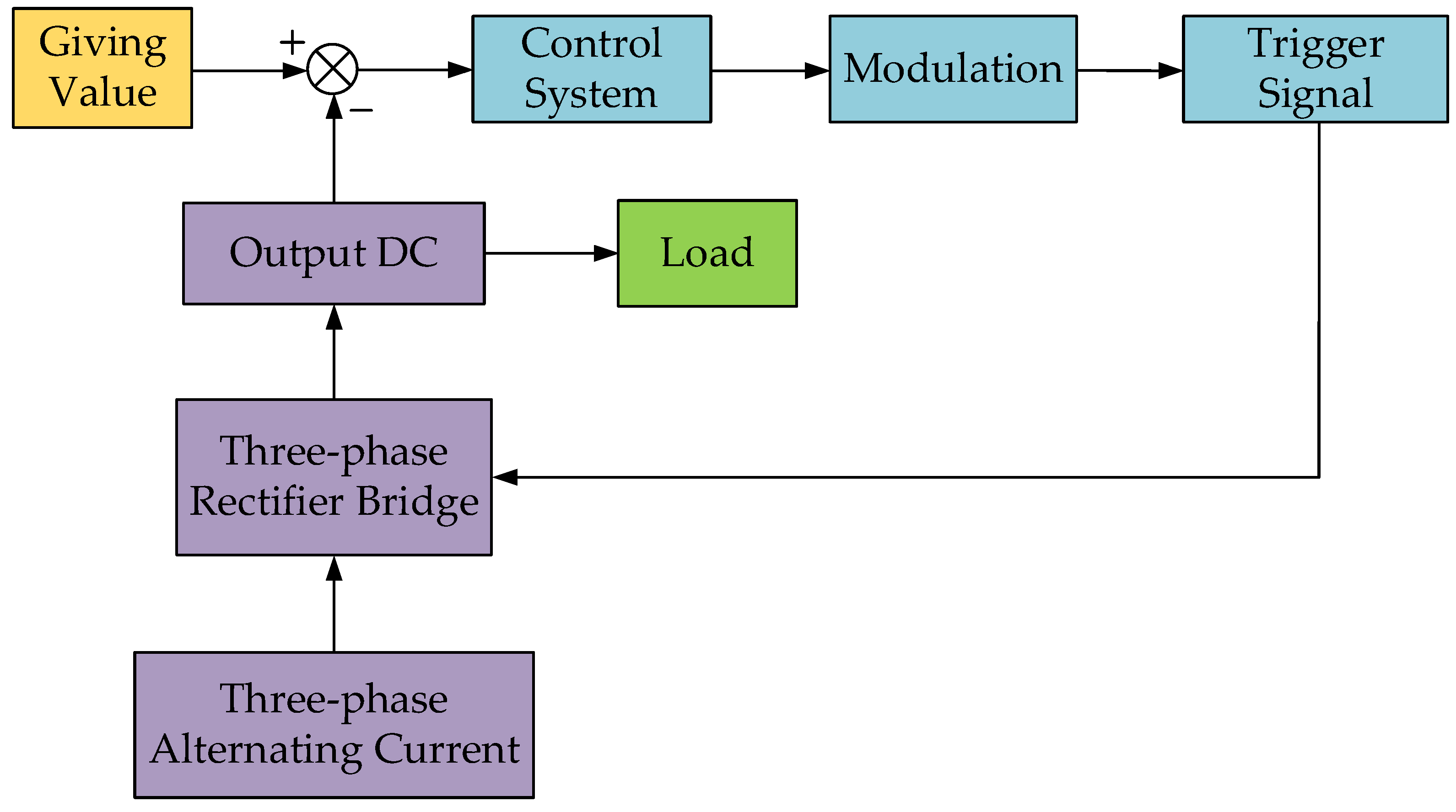
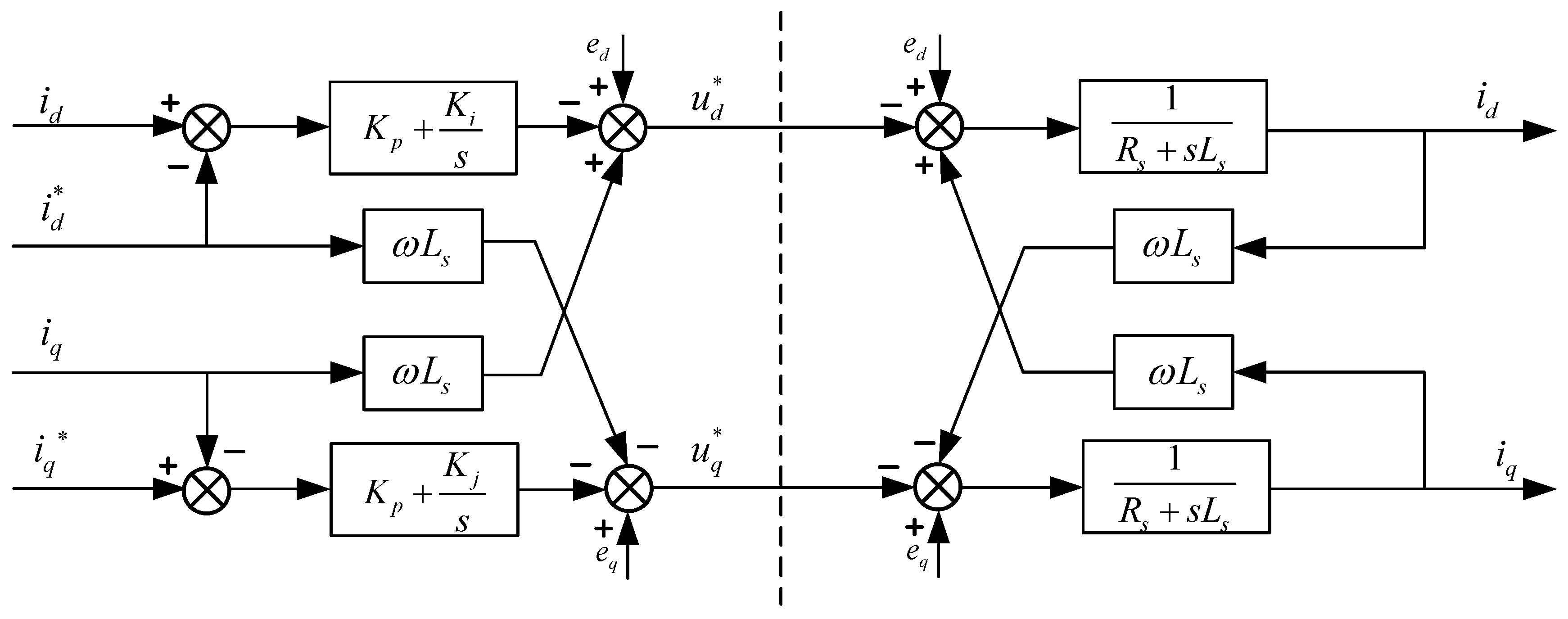
2.2. Controller Design

With $u_d$, $u_q$ as output and $i_d$, $i_q$ as input, the PI controller is used for control. Considering the need for feedforward decoupling, it can be derived by combining Equation (22) so that:

$$\{\begin{array}{l}{u}_d=(i_d-i_d^{*})(K_p+\frac{K_i}{s})+\omega L_s{i}_q+e_d\\ u_q=(i_q-i_q^{*})(K_p+\frac{K_i}{s})-\omega L_s{i}_d+e_q\end{array}$$

(23)

where $K_p$ and $K_i$ represent the coefficient of proportion and integration for the PI controller, respectively.

Following Equation (23), a controller with an inner-current loop can be designed. The system-block diagram at this point is detailed in Figure 6:

As demonstrated in the figure, the current $i_d$ and $i_q$ constitute a closed loop of the system at this point. Nevertheless, the control system does not interact with the output voltage on the DC side. In other words, the voltage fluctuations on the DC side cannot be adjusted by the control system for the time being. Thus, a voltage-closed loop needs to be designed.

The voltage-closed loop also adopts the PI controller, with $i_d$ as output, the expected voltage $u_{dc}^{*}$ on the DC side as input, and the actual voltage $u_{dc}$ on the DC side as feedback. Therefore,

$$i_d=(K_p{}^{\prime }+\frac{K_i{}^{\prime }}{s})(u_{dc}^{*}-u_{dc})$$

(24)

The voltage-closed loop is the largest and outermost control loop, which encloses the current-closed loop. Thus, it is called the outer-voltage loop, while the current-control change derived above is called the inner-current loop. The entire system diagram of the three-phase PWM rectifier is exhibited in Figure 7.

The outer-voltage loop is used to keep the DC-side voltage of the rectifier constant. Since the rectifier needs to maintain unit-power-factor operation, the reactive current ($i_q$) is set as 0. Next, $i_d$ (active current) and $i_q$ are compared with the feedback values of the current component on the dq-axis, respectively. Subsequently, the output performs a vector transformation after passing through the PI regulator. The result of the transformation is controlled by a space-vector modulator to control the switching tubes in the rectifier. Hence, the AC-side current waveform of the rectifier is sinusoidal, and the control effect can achieve unit-power-factor operation.

This control strategy has advantages such as its fast dynamic response, good steady-state performance, and built-in current-limiting protection. Since it can also eliminate current-steady-state errors and achieve unit-power factor [28], it can be applied across an extensive field of applications.

Additionally, a new stepped voltage-setting strategy is designed in this paper to achieve a better control effect. Detailed content is introduced in the control-strategy-improvement section of the report on the simulation analysis.

3. Simulation Analysis

Subsequently, a simulation in the MATLAB Simulink simulation module was established to verify whether the establishment of the above model was correct. The load in the DC side was 30 $\mathsf{\Omega }$, and it mutated to 15 $\mathsf{\Omega }$ at 0.25 s.

The most commonly used control method is to adopt voltage outer-loop and current inner-loop control. Through the current inner loop, the open-loop-transfer function of the current loop can be obtained, followed by the PI parameters. The open-loop transfer function of the voltage outer loop can be realized through the closed-loop-transfer function of the current inner loop, and the PI parameters of the voltage outer loop can be calculated [29]. Based on this parameter, further fine-tuning is performed to obtain the optimal parameters. The PI parameters in this paper are also tuned using this method. However, the calculated parameters can only serve as the initial values of the controller. It is crucial to further adjust the PI parameters to derive the desired results according to the issues in the output DC-voltage response. With the initial values calculated, the PI parameters are further fine-tuned by comparing the simulation results under different parameters to obtain a more ideal DC-voltage waveform. Relevant circuit parameters are listed in

Table 1. Circuit parameters.

Serial Number	Circuit Parameter	Value	Serial Number	Circuit Parameter	Value
1	Effective voltage value	380 V	6	Voltage outer loop $K_p$	0.85
2	Voltage frequency	50 Hz	7	Voltage outer loop $K_i$	50
3	${\mathrm{R}}_s$	40 $\mathrm{m}\mathsf{\Omega }$	8	Current inner loop $K_p$	10
4	${\mathrm{L}}_s$	1 mH	9	Current inner loop $K_i$	25
5	DC-side capacitance	6800 uF	10	Run time	0.4 s

.

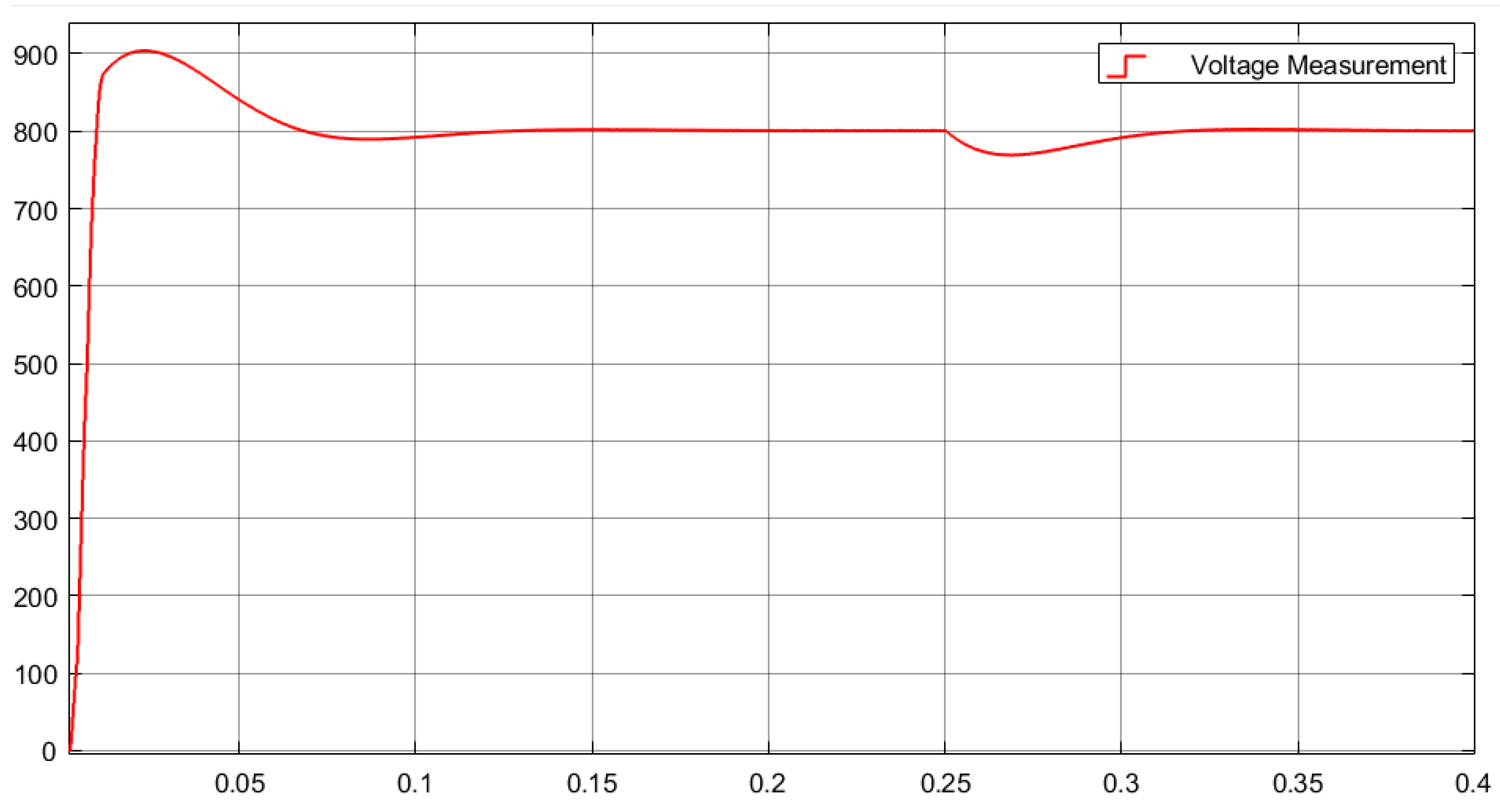
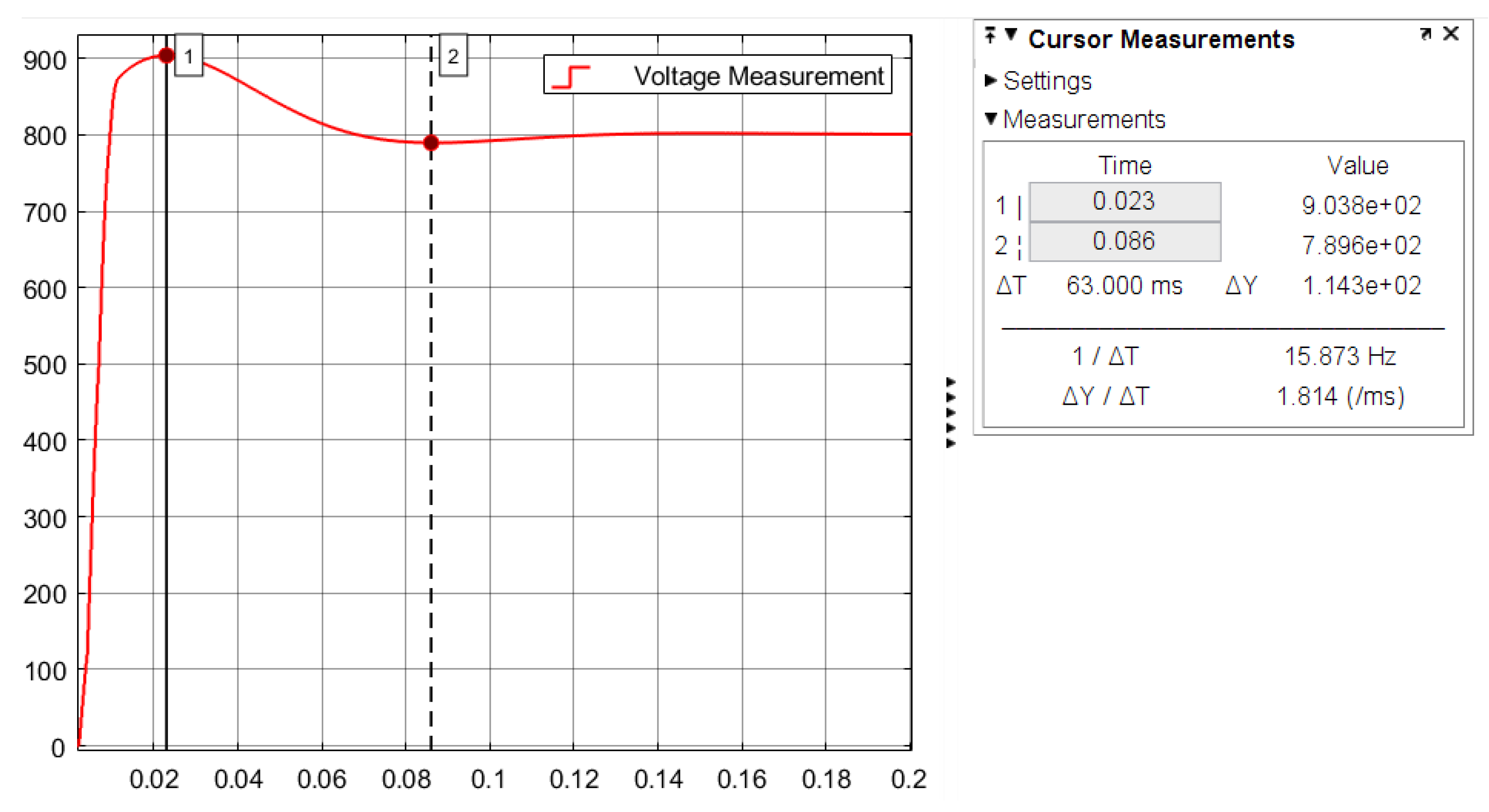
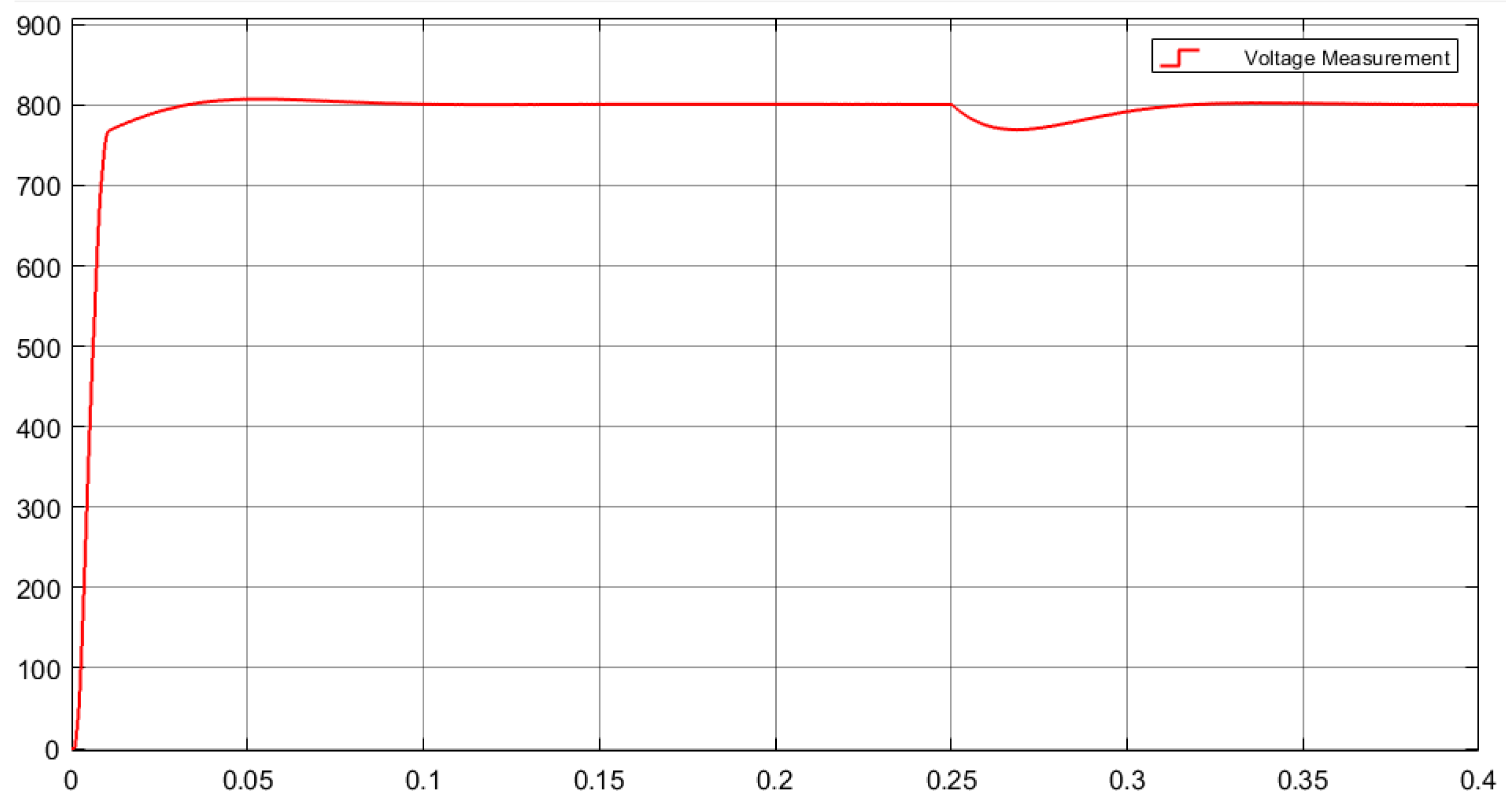
3.1. DC-Side Voltage Waveform

The output voltage waveform of the DC side obtained after running the simulation is drawn in Figure 8. The figure demonstrates that the DC side voltage can enter the 3% error band (800 ± 24 V) within 0.058 s and maintain stable operation when the output voltage of the derived double-closed-loop control system is given as 800 V and the PID parameter is selected as the value set above. The output voltage was affected when the load-resistance value changed abruptly at 0.25 s while automatically adjusting to the given value within 0.052 s and continuing to run statically. The overall control effect was ideal, in line with our expectations.

3.2. Analysis of Voltage and Current Waveform on the Grid-Side

An oscilloscope was employed to observe the single-phase voltage and current waveform on the grid side, as presented in Figure 9. At 0.25 s of simulation, the load-resistance value suddenly decreased by half, leading to an increase in the current amplitude. However, the current waveform on the grid side was very close to the sine wave, and the distortion degree was very low. Meanwhile, the voltage and current of the grid side almost always remained in the same phase, indicating that the unit-power-factor operation was maintained, resulting in slight pollution on the grid side. This also verified the advantages of the PWM rectifier described at the beginning of this article.

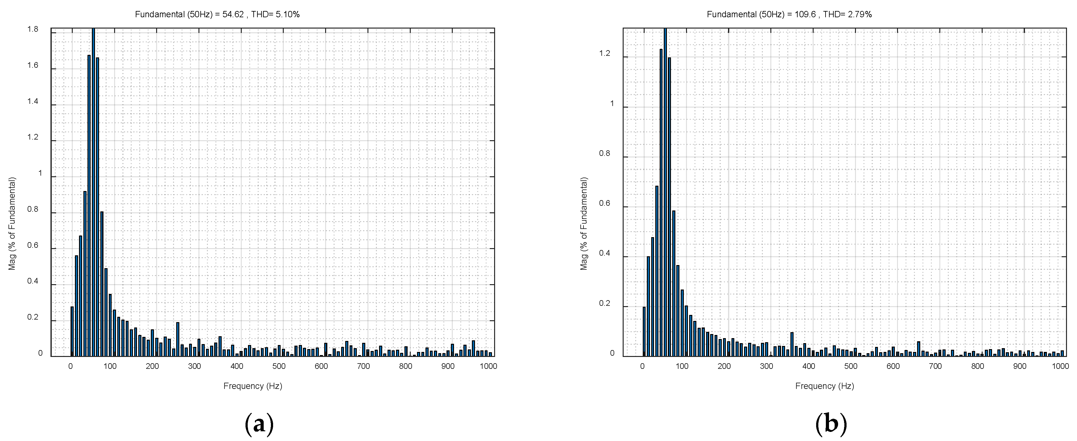
3.3. Analysis of Harmonic Content of Grid-Side Current

Although it is difficult to observe the distortion of the current waveform on the grid side in Figure 10, the resistance value was completely different under positive and reverse voltages due to the physical characteristics of the rectifier device. Hence, the current drawn by the rectifier from the power grid was also non-sinusoidal. The non-sinusoidal degree of the grid-side current varied from high to low owing to different circuit parameters, rectifier phase numbers, and other conditions. Such non-sinusoidal current waveforms can be decomposed into the fundamental wave and a series of harmonics with different frequencies and amplitudes. The total content of these harmonics represents not only the distortion degree of the whole waveform but also the performance of the rectifier. Therefore, the FFT-analysis module in Simulink was utilized to measure the THD (total harmonic distortion) of the current at the grid side.

The grid-side current with load-resistance changes after 0.25 s was taken as the typical current, and the THD-measurement results are presented in Figure 10. The simulation results under more load conditions are detailed in

Table 2. THD values under different loads.

Serial Number	$\mathbf{Load} \mathbf{Value}/\mathsf{\Omega }$	THD	Serial Number	$\mathbf{Load} \mathbf{Value}/\mathsf{\Omega }$	THD
1	10	1.86%	5	30	5.10%
2	15	2.79%	6	35	5.66%
3	20	3.58%	7	40	6.48%
4	25	4.02%	8	50	8.15%

. The results revealed that the THD value increased with the increase in the load-resistance value, exceeding 5% at a load of 30 $\mathsf{\Omega }$. Methods such as improving the coordinate-rotation algorithm can be employed to curtail the harmonic content [30].

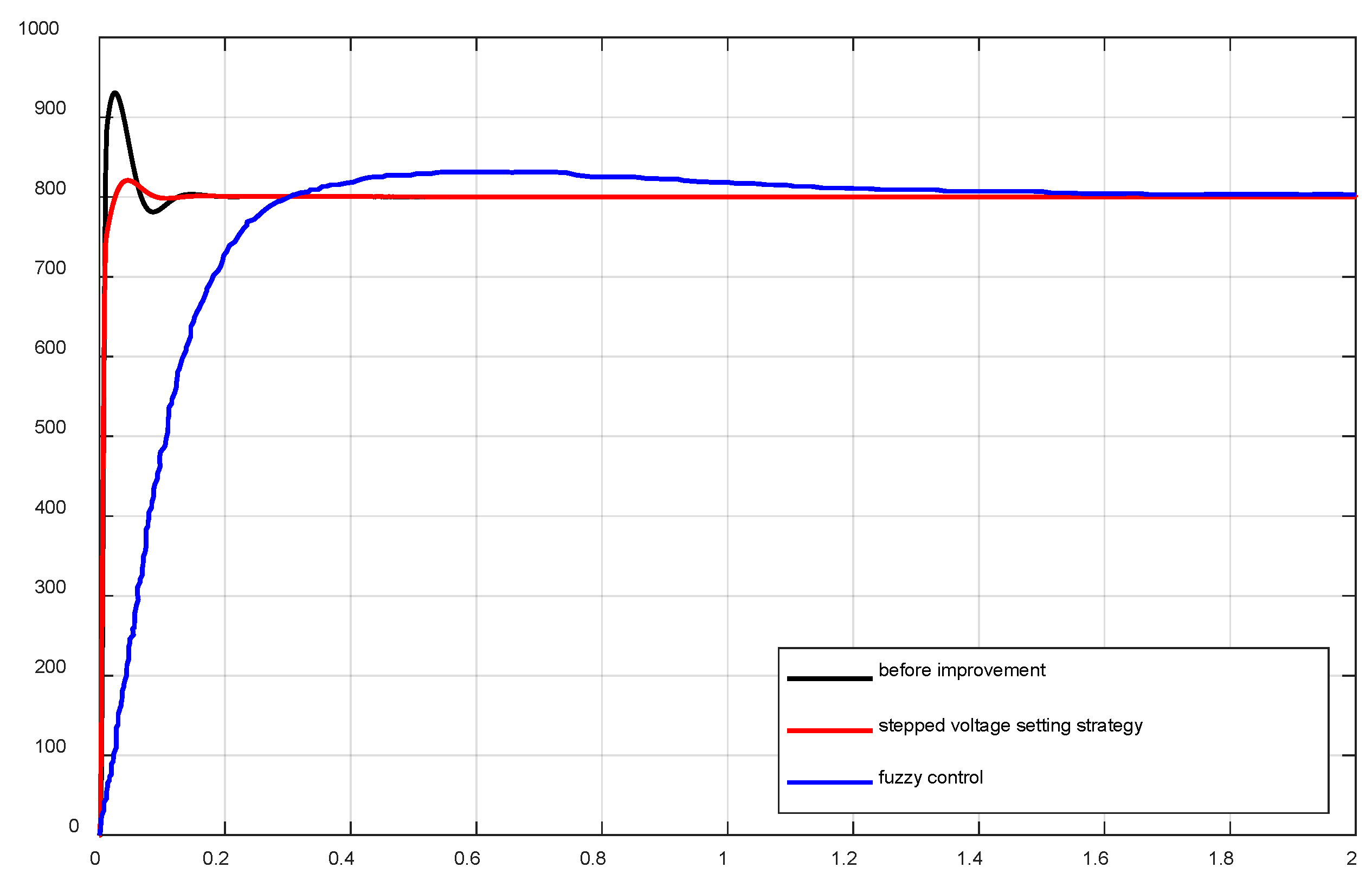
3.4. Control-Strategy Improvement

Figure 11 illustrates that although the overall control effect was consistent with expectations, there was an excessive overshoot in the start-up stage. When using the measurement function in the Simulink oscilloscope, the peak voltage was about 903 V at peak time $t_p=0.023\mathrm{s}$. Therefore, the system overshoot was:

$$\sigma \%=\frac{c_{\max }-c(\infty )}{c(\infty )}\times 100\%=\frac{903-800}{800}\times 100\%=12.88\%$$

(25)

Since the overshoot is large, the control strategy should be improved. At present, many strategies offer ideal improvement effects, involving the use of a voltage square ring as the outer ring and the adoption of the capacitor current on the DC side started by the rectifier as the reactive current-control method [31]. Furthermore, the fuzzy algorithm is utilized to enhance the dynamic performance and system robustness [32,33]. However, the control-system structure in this method is complicated, the readability is poor, and the maintenance cost of the rectifier is increased. Therefore, a simple and easy-to-control starting method is designed in this paper to tackle the problem of overshooting when the rectifier starts.

When starting, the analysis implies that the rectifier is in an uncontrollable rectifier state, and its maximum output voltage on the DC side is:

$$u_{dc}=\frac{3}{\pi }{\displaystyle {\int }_{\frac{\pi }{3}}^{\frac{2\pi }{3}}\sqrt{6}{U}_m\sin (\omega t)d(\omega t)}=2.34U_m$$

(26)

The $U_m$ denotes the effective value of the phase voltage on the side of the grid.

In normal operations, the minimum output voltage is:

$$u_{dc}=\sqrt{6}{U}_m=2.45U_m$$

(27)

Given the large capacitor on the DC side, the voltage cannot mutate, and the rectifier inevitably modulates excessively, resulting in an overshoot of the output voltage [20].

Therefore, the stepped voltage-setting strategy is adopted in this paper. Specifically, the given voltage of the DC side of the rectifier is input in the form of a step increase, rather than direct full-voltage input. The electrical impact caused by the sudden switch from a stationary state to a high-voltage state can be reduced by giving the voltage value in steps. Specifically, although the feedback voltage on the DC side at the starting moment is 0, the given voltage at this point is also a small value. As a result, the input-error value is not excessively large, and the intensity of the regulation of the control system is not excessively high. In a short period of time, if no other actions are undertaken, the output voltage of the rectifier will reach the given small voltage and then exceed this value, reach the peak value, and finally fall back to the given small voltage. Nevertheless, this part of the overshoot can be utilized as long as the given voltage value is controlled in a timely manner so that it changes from a small voltage to the original full voltage at the appropriate time. In this way, the rectifier can smoothly track the given voltage value without a noticeable overshoot.

The selection of the point at which the given voltage jump occurs should follow two principles. Firstly, the rectifier output voltage should reach its peak before the value is small. Second, if the peak output voltage at a given value of low voltage exceeds the actual full voltage, it should jump before reaching full voltage. In the latter case, the low voltage value can be adjusted first. If the full voltage is exceeded within the range of $20\%~50\%U_{*}$, the jump time can be adjusted.

With the same simulation model, the parameters above were given by the MATLAB programming function to join a stepwise growth module, so as to validate the control effect and the feasibility of a given strategy. Its initial value was set as $0.4U_{*}$ and the jump into $U_{*}$ occurred at 0.0057 s ; in other words, the jump into total voltage occurred after 0.0057 s. The DC-output-voltage waveform is depicted in Figure 12.

Figure 12 demonstrates that the waveform of the rectifier startup was much more stable than that before the improvement, and that the overshoot was significantly suppressed. The starting point was locally magnified, and its peak voltage was measured with the measuring function of the oscilloscope. The results are presented in Figure 13.

The figure suggests that the peak voltage was 807.4 V. The overshoot at this point is expressed as:

$$\sigma \%=\frac{c_{\max }-c(\infty )}{c(\infty )}\times 100\%=\frac{807.4-800}{800}\times 100\%=0.925\%$$

(28)

Compared with the 12.88% before the strategy was improved, the control effect was significantly better.

In addition to the two-layer growth shown in this paper, a given voltage can also be increased in multiple layers. Specifically, multiple jumps occur in a given voltage , with values a little larger than the previous values each time; finally, the actual total voltage is reached. A function can be utilized to control a given voltage for changes over time. However, the simulation revealed that the control effect of these strategies was not considerably improved, and some methods even led to an overshoot increase instead of a decrease. Therefore, the simplest and most effective second-order jump was employed in this paper.

At present, there are many improvement strategies for starting overvoltage, such as fuzzy control and voltage-square loop, which are widely used. Nonetheless, the control method of voltage-square loop increases the harmonic content of the system (using the method in [28], the THD value reaches 13.93%), as well as the complexity and cost of the system. Given its small voltage range, which is different from the applicable range of this article, it is not compared in Figure A1. Fuzzy control is often used in PV systems to achieve maximum power. The authors of [16] improved fuzzy control, enabling the controller to show more stable behavior. These findings all indicate the enormous potential of fuzzy control in certain specific fields. Furthermore, many studies also apply fuzzy control to three-phase PWM rectifiers, but the results demonstrate that it cannot handle rapidly changing systems, and it is also difficult to explain and understand the operating mechanism of fuzzy control. A comparison of the simulation results obtained after changing the load to the same value as in [29] is exhibited in Figure A1. It can be observed that the stepped voltage-setting strategy proposed in this paper has a fast response speed, small voltage overshoot, and better control effect.

4. Conclusions

The three-phase PWM rectifier has a wide range of applications in the field of power electronics, and the improvement of its control strategy has long been a research focus. In this paper, we deduced the input-and-output mathematical model of a three-phase PWM rectifier, established its simulation model in Simulink, and then simulated and validated the widely used dual voltage-and-current closed-loop control strategy. By analyzing the simulation results, the following conclusions can be drawn:

(1)

The control strategy has a short start-up time and good dynamic performance, and it can automatically and quickly track back to a given value when the load changes;

(2)

The control strategy can sinusoidize the network-side current, reduce the harmonic pollution on the network side, and operate in the state of unit-power factor;

(3)

The DC-side output-voltage overshoot was large at startup, and the simulation result was 12.88%.

To solve this problem, a stepped voltage-setting strategy was proposed, and its validity in starting-voltage-overshoot suppression was verified by a simulation. The strategy reduced the overshoot to 0.925%. Compared with traditional control strategies, such as fuzzy control, this method is more operable, its use is more flexible, and it has a shorter start-up time.

However, there are still shortcomings in the current research on the double-closed-loop control of PWM rectifiers. For example, the system-response time is overly long when the given voltage is less than approximately 600 V; furthermore, the voltage overshoot is excessively large and almost uncontrollable when the given voltage is greater than approximately 1100 V. Therefore, the detailed mathematical relationship between the load values, given voltage, and voltage-step time needs to be derived in future research to improve the effective voltage-control range of three-phase PWM rectifiers, rendering their dynamic and static performance more ideal and more flexible in practical applications.

References

1. Zhang, H.; Jin, R.; Zhao, Y.; Jiang, J.; Wang, A. Simulink Simulation Analysis of Single-phase Half Wave Controlled Rectifier under Different Load Conditions. Res. Explor. Lab. 2022, 41, 105–109. [Google Scholar]
2. Cao, Y.; Shi, J.; Shi, X.; Liu, Y.; Liu, M. Exploration in One-Way Full-Wave Rectification Experiment Teaching Based on Analog Simulation. Mod. Inf. Technol. 2022, 6, 192–195. [Google Scholar]
3. Wang, S.; Zhou, Y. Analysis on Active Power of a Three-phase Half-wave Controlled Rectifier with Resistor-Inductor Load in Intermittent State. Power Equip. 2017, 31, 240–244+249. [Google Scholar]
4. Zhao, R.; He, Y.; Liu, Q. Research on Improvement of Anti-Disturbance Performance for Three-Phase PWM Rectifiers. Trans. China Electrotech. Soc. 2004, 19, 67–72. [Google Scholar]
5. Zhang, L.; Zhao, J.; Shao, T.; Ma, R. Implement Waveform and Phase Control of Grid Side Current Based on PWM Rectifier. Available online: http://design.eccn.com/design_2022052709091520.htm2022/2023 (accessed on 27 May 2022).
6. Abdollahi, R.; Gharehpetian, G.B.; Mohammadi, F.; Prakash, P.S. Multi-Pulse Rectifier Based on an Optimal Pulse Doubling Technique. Energies 2022, 15, 5567. [Google Scholar] [CrossRef]
7. Corti, F.; Hassan Shehata, A.; Laudani, A.; Cardelli, E. Design and Comparison of the Performance of 12-Pulse Rectifiers for Aerospace Applications. Energies 2021, 14, 6312. [Google Scholar] [CrossRef]
8. Li, T.; Gan, Y. Hybrid Modulated DCDC Boost Converter for Wearable Devices. Electronics 2022, 11, 3418. [Google Scholar] [CrossRef]
9. Almutairi, A.; Sayed, K.; Albagami, N.; Abo-Khalil, A.G.; Saleeb, H. Multi-Port PWM DC-DC Power Converter for Renewable Energy Applications. Energies 2021, 14, 3490. [Google Scholar] [CrossRef]
10. Fatma, M.; Hamid, M. PWM speed control of dc permanent magnet motor using a PIC18F4550 microcontroller. IOP Conf. Ser. Mater. Sci. Eng. 2019, 602, 012017. [Google Scholar] [CrossRef]
11. Li, Y. Design of PWM Speed Regulation System for DC Motor Based on ARM. Eng. Test 2022, 62, 108–110. [Google Scholar]
12. Koc, B.; Kist, S.; Hamada, A. Wireless Piezoelectric Motor Drive. Actuators 2023, 12, 136. [Google Scholar] [CrossRef]
13. Surakasi, B.; Satish, R.; Pydi, B.; Kotb, H.; Shouran, M.; Abdul Samad, B. A NovelMethodology to Enhance the Smooth Running of the PM BLDC Motor Drive Using PWM-PWM Logic and Advance Angle Method. Machines 2023, 11, 41. [Google Scholar] [CrossRef]
14. Venkatesan, M.; Rajamanickam, N.; Vishnuram, P.; Bajaj, M.; Blazek, V.; Prokop, L.; Misak, S. A Review of Compensation Topologies and Control Techniques of Bidirectional Wireless Power Transfer Systems for Electric Vehicle Applications. Energies 2022, 15, 7816. [Google Scholar] [CrossRef]
15. Huang, R. The Research of the Application of the AC Charging System of Electric Vehicles in the New Energy Vehicle Technology Major. Auto Time 2023, 2, 113–115. [Google Scholar]
16. Samavat, T.; Nazari, M.; Ghalehnoie, M.; Nasab, M.A.; Zand, M.; Sanjeevikumar, P.; Khan, B. A Comparative Analysis of the Mamdani and Sugeno Fuzzy Inference Systems for MPPT of an Islanded PV System. Int. J. Energy 2023, 2023, 7676113. [Google Scholar] [CrossRef]
17. Ikeda, F.; Okamoto, M.; Hamasaki, K.; Yamada, H.; Tanaka, T. Constant DC-Capacitor Voltage-Control-Based Reactive Power Control Method of Bidirectional Battery Charger for EVs in Commercial Single-Phase Three-Wire Low-Voltage Feeders: Special Issue Paper. IEEJ J. Ind. Appl. 2021, 10, 761–769. [Google Scholar] [CrossRef]
18. Rastgoo, S.; Mahdavi, Z.; Azimi Nasab, M.; Zand, M.; Padmanaban, S. Using an Intelligent Control Method for Electric Vehicle Charging in Microgrids. World Electr. Veh. J. 2022, 13, 222. [Google Scholar] [CrossRef]
19. Zhang, C.; Zhang, X. PWM Rectifier and Its Control; China Machine Press: Beijing, China, 2003; pp. 3–5, 51–65. [Google Scholar]
20. Pathak, P.K.; Yadav, A.K.; Tyagi, P. Design of Three Phase Grid Tied Solar Photovoltaic System Based on Three Phase VSI. In Proceedings of the 2018 8th IEEE India International Conference on Power Electronics (IICPE), Jaipur, India, 13–15 December 2018; pp. 1–6. [Google Scholar] [CrossRef]
21. Wu, F.J.; Sun, D.Y.; Duan, J.D. Diagnosis of single-phase open-line fault in three-phase PWM rectifier with LCL filter. IET Gener. Transm. Distrib. 2016, 10, 1410–1421. [Google Scholar] [CrossRef]
22. Jiang, W.; Li, W.; She, Y. Control Strategy for PWM Rectifier Based on Feedback of the Energy Stored in Capacitor and Load Power Feed-Forward. Trans. China Electrotech. Soc. 2015, 30, 151–158. [Google Scholar]
23. Cai, S.; Cao, H.; Liang, D.; Niu, R.; Jia, L.; Waseem, A. A three-phase voltage source PWM rectifier with strong DC Immunity based on model predictive control. In Proceedings of the 34th Chinese Control Conference, Hangzhou, China, 28–30 July 2015; pp. 7871–7876. [Google Scholar]
24. Zhong, C.; Du, H.; Yang, M. Analysis of Starting Inrush Current of Three-phase Unity Power Factor VSR and Its Suppression. Power Electron. 2013, 47, 32–34. [Google Scholar]
25. Zhang, X. Research on PWM Rectifier and Its Control Strategy. Ph.D. Thesis, Hefei University of Technology, Hefei, China, 2003. [Google Scholar]
26. Lang, Y.; Xu, D.; Hadianamrei, S.; Ma, S. Improved feedforward control of three-phase voltage source PWM rectifier. Electr. Mach. Control. 2006, 10, 160–170. [Google Scholar]
27. Huang, Q.; Tang, J.; Lin, L.; Liu, X.; Zhang, Y. Research on a kind of inner and outer loop decoupling control for three-phase voltage-source PWM rectifier. J. Shaoyang Univ. (Nat. Sci. Ed.) 2020, 17, 40–47. [Google Scholar]
28. Li, D.; Shi, X. Simulation of Three·phase Voltage Source PWM Rectifier and Its Control Strategy. Control Inf. Technol. 2010, 3, 19–23. [Google Scholar]
29. Zhou, Q.; Liang, H. The Design and Analysis of PI Regulator of Three-phase Voltage Source Rectifier. Power Electron. 2011, 45, 50–52. [Google Scholar]
30. Zhu, Y.; Wang, Z.; Wang, C.; Zhu, Y.; Cao, X. A Novel Improved Coordinate Rotated Algorithm for PWM Rectifier THD Reduction. Electronics 2022, 11, 1435. [Google Scholar] [CrossRef]
31. Yao, X.; Wang, X.; Feng, Z. Research on of Improvement of the Dynamic Ability for PWM Rectifier. Trans. China Electrotech. Soc. 2016, 31, 169–175. [Google Scholar]
32. Jiang, L. Application of Fuzzy Control in Three-phase PWM Rectifier. J. Lanzhou Univ. Arts Sci. (Nat. Sci.) 2022, 36, 29–33. [Google Scholar]
33. Yao, Q.; Zeng, G.; Huang, B.; Liu, J.; Wei, Y. Control strategy design of three-phase PWM rectifier based on variable universe fuzzy PI. Manuf. Autom. 2022, 44, 73–76. [Google Scholar]
Figure 1. The overall framework of the model.
Electronics 12 02417 g001
Figure 2. Topology of the main circuit of the three-phase bridge rectifier.
Electronics 12 02417 g002
Figure 3. Coordinate-transformation-comparison diagrammatic sketch. (a) Vector schematic figure in three-phase static coordinate system. (b) Vector schematic figure in two-phase static coordinate system.
Electronics 12 02417 g003
Figure 4. Diagram of the relationship between different angles.
Electronics 12 02417 g004
Figure 5. Schematic diagram of input-and-output mathematical model of PWM rectifier.
Electronics 12 02417 g005
Figure 6. Part of the system-block diagram.
Electronics 12 02417 g006
Figure 7. Three-phase PWM-rectifier-control-strategy-structure diagram.
Electronics 12 02417 g007
Figure 8. DC-output-voltage waveform.
Electronics 12 02417 g008
Figure 9. Voltage and current waveform on grid side.
Electronics 12 02417 g009
Figure 10. Analysis diagram of the harmonic content of grid-side current under different loads. (a) Load is 30; (b) load is 15.
Electronics 12 02417 g010
Figure 11. The output-voltage waveform on the DC side at startup.
Electronics 12 02417 g011
Figure 12. Improved DC-side-voltage waveform.
Electronics 12 02417 g012
Figure 13. Improved DC-side-voltage waveform (partially enlarged).
Electronics 12 02417 g013