Forecasting Carbon Dioxide Emissions of Light-Duty Vehicles with Different Machine Learning Algorithms

Abstract

Accurate estimation of fuel consumption and emissions is crucial for assessing the impact of materials and stringent emission control techniques on climate change, particularly in the transportation industry, which accounts for a significant portion of global greenhouse gases and hazardous pollutants emissions. To address these concerns, the government of Canada has collected a large sensor-based dataset containing detailed information on 7384 light-duty vehicles from 2017 to 2021, with the goal of reducing CO₂ emissions by 40–45% by 2030. To this end, various researchers worldwide have developed vehicle emissions and consumption models to comply with these targets and achieve the Canadian government’s ambitious objectives. In this work, we propose the development of boosting and other regression models to predict carbon dioxide emissions for light-duty vehicle designs, with the aim of creating ensemble learning models that leverage vehicle specifications to forecast emissions. Our proposed boosting model is capable of accurately predicting CO₂ emissions, even with only one car attribute as input. Moreover, our regression models, in conjunction with the boosting algorithm, can effectively make predictions from various vehicle inputs. Our proposed technique, categorical boosting (Catboost), provides critical insights into transportation-generated air pollution, offering valuable recommendations for both vehicle users and manufacturers. Importantly, Catboost performs data processing in less time and with less memory than other algorithms proposed in the literature. Future research efforts should focus on developing higher performance models and expanding datasets to further improve the accuracy of predictions.

1. Introduction

Environmental challenges created by transportation have become more complicated with the fast rise in urbanization because of significant changes in climatic conditions all over the world [1]. Seventy-five per cent of all carbon dioxide emissions come from passenger cars, which are also liable for 20 to 30 per cent of all global greenhouse gas (GHG) emissions [2]. Despite rigorous GHG and fuel standards, the quantity of used cars has also increased [3,4]. The increase in vehicles, vehicle miles and travelled (VMT) has resulted in high air pollutant emissions and natural resource consumption from old cars [5]. The transportation industry is a crucial component of many daily activities, including passenger movement and the sustainable supply of goods. However, the industry has maintained sustainability by using internal combustion engines to consume fossil fuels [6].

The transportation industry consumes more than half of the world’s oil production, which hastens the depletion of fossil fuel sources. Fuel costs have gradually increased because of the transportation industry [7]. The world has seen increases in the transportation sector. As a result, the transport sector is liable for around a quarter of all anthropogenic CO₂ emanations worldwide. The transportation segment includes light-duty vehicles. A light-duty vehicle is any mobile device with a gross vehicle weight rating of less than or equal to 10,000 pounds primarily used to transport people and goods. Examples include automobiles, vans, SUVs, and pickup trucks. In the modern world, it is more evident how the carbon footprint affects human health and how energy use affects the growth of a country’s economy. Therefore, national economic issues have been the main problem for federal policymakers during the past few decades [8].

There has been an increase in energy demand with social and economic advancements. Every country’s socioeconomic development, urbanization, and population growth are all expanding quickly [9]. Carbon emissions impact human health in two ways, that is, directly and indirectly [10]. High carbon emissions immediately affect people’s respiratory systems. The respiratory system health issues will result in shortness of breath, headaches, dizziness, weakness, and delirium. The indirect impact of carbon on humans is contributes to significant global problems, including global warming, climate change, and acid rain [11]. In addition to carbon emissions, the transportation industry produces considerable amounts of PM_2.5, PM₁₀, SO₂, N₂O, etc., so these issues are significant to the environment and people [12]. The best way of solving this problem is by controlling the release of carbon and by lessening the effect of carbon.

Calculating the cost of energy and air pollution caused by vehicles depends on estimating and visualizing fuel consumption and carbon emissions [13]. Forecasting models of CO₂ emissions and automobile fuel consumption are becoming more critical as climate variation has become a major problem over the past ten years. Because of this, researchers and engineers worldwide are more interested in data analytics and machine learning techniques for creating a sustainable environment [14]. Researchers have developed machine-learning models and methodologies for estimating carbon dioxide emissions [15,16]. Comparing various vehicle types and their environmental impact is essential for the car market. Such research offers a profound understanding of the effects of vehicles on the environment. The proposed work will fill the highlighted gap through meticulous data analyses and machine learning by providing a vision of vehicle petroleum utilization and carbon dioxide emission.

The study analyzes current trends in CO₂ releases by various vehicle brands and models. This paper represents a complete systematic review of fuel usage and carbon dioxide emissions for the latest light-duty automobiles. The data preparation process of the dataset is also discussed in this paper. An analytical and predictive study using 7384 light-duty vehicles spotted from 2017 to 2021 from the government of Canada dataset has been performed to execute and address the specified research objectives. Two statistical means of data analysis are used in this study: (1) a descriptive statistical analysis to evaluate the fuel efficiency and CO₂ emissions of light-duty automobiles and (2) an inferential statistical analysis based on various properties of vehicles to determine the relationship between all dataset attributes. The main goal is to create machine learning models that predict carbon dioxide emissions and fuel consumption based on vehicle characteristics data.

2. Related Works

Vehicle emissions can be divided into two main groups: the ones that are harmful to the environment and human health and the ones that accelerate climate change. Carbon dioxide (CO₂) emissions, which account for the majority of greenhouse gas (GHG) emissions, are the ones that have the most significant impact on climate change. In the European Union, road traffic contributes to one-fifth of all carbon dioxide emissions, with passenger automobiles accounting for 75% of these emissions [17]. Furthermore, there is a clear and significant correlation between gasoline usage and CO₂. The average fleet emission limitations in the European Union (EU) are given in terms of CO₂ emissions, expressed in grammes per kilometer. Similar methods have been employed in North America, but with restrictions on fuel economy [18]. The decarbonization of the transportation sector must start with electric automobiles. However, according to the International Energy Agency, to keep global warming below 2 °C by 2030, at least 20–25% of all highway transport vehicles must be motorized by electric energy (approximately 300 million cars) [19]. To prevent the worst effects of climate change, the government of Canada has likewise committed to attaining net-zero emissions by 2050. It has set the goal of lowering emissions by 40–45% by 2030. Therefore, numerous academics worldwide have suggested that various vehicle emissions and consumption models satisfy those CO₂ limit criteria and meet such high statutory standards [20].

Researchers have developed several models for estimating car emissions during the past few decades. A micro-scale model called CORSIM is constructed using tables to estimate emissions based on dynamometer data. The CORSIM technique affects default release rates per one second depending on the acceleration and speed of each vehicle that travels on the specified link to calculate the total emissions of each link [21]. The EMIT model uses a regression equation with acceleration and speed to estimate CO₂, CO, and nitro oxide emissions and is based on dynamometer data from 344 light-duty vehicles. In 2010, a US government agency developed the MOVES model for project- or region-level greenhouse gas emissions calculations, including carbon oxide, nitro oxide, VOC_s and PM from light-duty automobiles. A model for calculating CO₂ emissions using instantaneous vehicle power by factoring in elements, including total resistance force, vehicle mass, speed, and driveline performance, is developed [22].

The Georgia Institute of Technology’s “MEASURE” illustrates the use of data-intensive parameters. It computes the carbon oxide, nitro oxide, and VOC emissions from all automobile operating modes, such as deceleration, cruise control, acceleration, and idle. Despite having more than 30 features as inputs, this model must account for CO₂ estimation [23]. The European Environment Agency (EEA) created another well-known framework called COPART, which has since become one of the normative approaches for road conveyance emission records in EEA member nations [24]. Constructing the links between national natural energy consumption and release patterns is a significant area of research. Additionally, several recent authors have used machine learning and deep learning techniques for predicting car CO₂ emissions. A model that forecasts the NOx and CO₂ emissions from heavy-duty trucks using artificial neural networks was proposed by using the U.S. environmental protection agency (EPA) dataset. Although the result is favorable, CO₂ has yet to be considered, and the model is suitable for gasoline-powered cars [25]. After testing 70 diesel automobiles under real-world driving situations, a team of researchers used a machine learning model to predict emissions along with vehicle performance. For instantaneous NOx forecasts, look-up tables, non-linear regression (NLR), and neural network multilayer perceptron (MLP) models are accordingly used. Although the model considers the vehicle’s acceleration and speed, its outputs are limited to NOx estimation, and CO₂ is left out [26]. Traditional ANN does not draw conclusions about the subsequent information based on prior knowledge. Recurrent neural networks (RNNs), which contain loops that permit data to persist, address this problem. Since the backpropagation method was used to train RNN, it was possible that the gradient would approach 0 or infinity when the networks were deep. Special RNNs called long short-term memory networks (LSTMs) are used to solve gradient vanishing and clipping issues [27]. A proposed methodology that tested the prediction accuracy of different machine learning models on CO₂ emissions and Gaussian process regression (GPR) and obtained good results was carried out on real driving emission (RDE) data collected from hybrid electric vehicles. Additionally, it has been discovered that the CO₂ emissions of hybrid electric cars are not directly proportional to their acceleration and speed [28].

Numerous techniques, such as different algorithms and scientific models, have been investigated in the pertinent literature for trailing trends, modelling, and estimating CO₂ emissions. Overall, the research involved in the forecasting of CO₂ emissions and energy demand for Canada and other nations has primarily concentrated on the appropriate countries’ overall natural energy utilization dataset. Although the quantity of this research is relatively small, it is nevertheless feasible to discover a few papers that forecast Turkey’s CO₂ and other GHG emissions using transportation information.

Table 1. An overview of the research on CO₂ emissions or energy usage.

Reference and Year	Technique	Dataset Period	Country	Input	Prediction Output	Performance Metric
[9] and 2021	Deep learning	1990 to 2018	Turkey	Energy and vehicle parameters	CO2 and energy demand	RMSE, MBE, RMSE, R2, and MAPE
[11] and 2021	ANN, DNN	2000 to 2018	Turkey	GDP, population, vehicle parameters	CO2	MAPE, RMSE, MAE
[25] and 2016	ANN	1994 to 1999	U.S. (EPA)	Energy and vehicle parameters	NO2, CO2	R2, slope, and interception
[26] and 2020	NLR, MLP	2012 to 2016	U.K.	Vehicle parameters	NO2, CO2	Fractional bias, normalized MSE
[27] and 2020	LSTM	2012 to 2017	Germany	Energy parameters	CO2	RMSE, R2, and MAPE
[28] and 2021	Regression models, neural net	2001 to 2013	California	Energy and vehicle parameters	CO2 and fuel consumption	RMSE, R2, and MAPE
[29] and 2017	Grey model	1965 to 2014	Turkey	Energy parameters	CO2	MAPE, MSE, and RMSE
[30] and 2021	Grey model	1978 to 2014	G-6 Countries	Vehicle parameters	CO2	MAE, MAPE, C C = error ratio
[31] and 2019	Regression models	1995 to 2016	Turkey	GDP, population, and energy	CO2	R2
[32] and 2017	Regression models	1970 to 2015	Iran	GDP, population, previous CO2 emission	CO2 and energy request	R2, MAPE, MAE, Standard deviation,
[33] and 2020	ANN	2005 to 2018	China	GDP, population, and energy	CO2	MAPE, RMSE, MAE
[34] and 2019	ANN	1975 to 2016	Turkey	Population, GDP, oil price, vehicle km	CO2 and energy request	R2, MAE, MAPE, RMSE, MSE
Current paper	Regression and boosting models	2017 to 2021	Canada	Vehicle parameters	CO2	R2, RMSE, MAE, Standard deviation

thoroughly describes earlier research on projecting CO₂ and energy consumption.

The literature shows that various methods have been commonly used to accurately forecast energy consumption and CO₂ emissions. According to the pertinent papers, there is a significant relationship between the energy demand and CO₂ emissions for the relevant regions and nations and the people, automobile kilometer, energy import and export, gross household product, oil amount, annual vehicle kilometer, historical CO₂, passenger kilometer, and chronological energy trends.

3. Materials and Methods

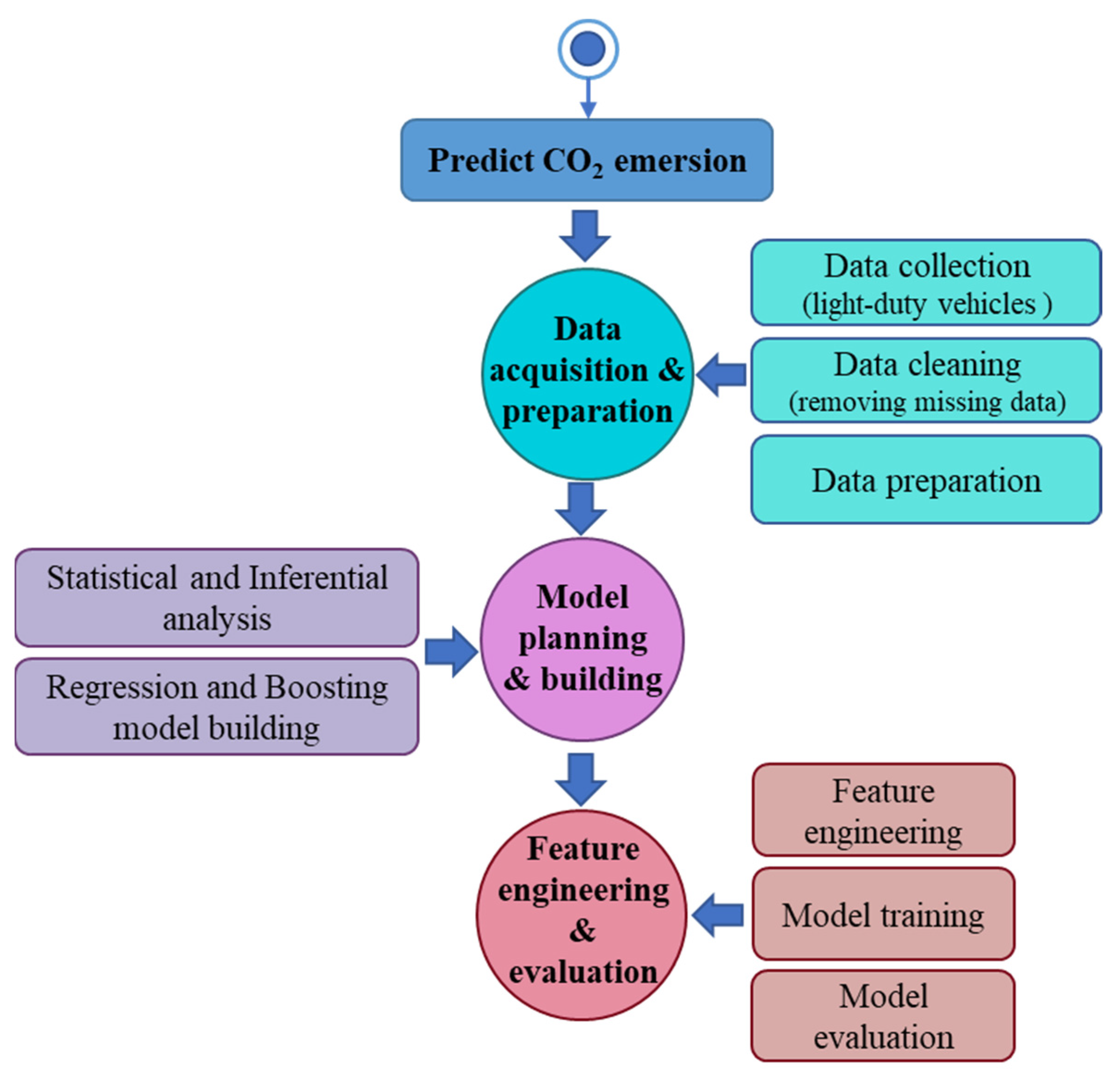
The government of Canada gathered the dataset in this analysis to undertake analytical and predictive research on car carbon dioxide releases. For this study, a data analytics life phase has been used. This life phase has four levels, typical for data science and big data analytics. Figure 1 demonstrates the life cycle of predicting CO₂ emission.

The life cycle is divided into four levels. Level 1 is discovering the issue and goals, which is the first step in this process. This research aims to provide a comparative analysis of carbon dioxide releases among various vehicle models and vehicle brands, make suggestions supported by the available data, and build a model that can predict changes in future emission rates. Level 2 is data acquisition and preparation. The dataset utilized in this analysis is drawn from the government of Canada’s “Fuel consumption rating” databases, which include measured CO₂ emissions and fuel consumption rankings for 7384 samples of light-duty cars in Canada. The information was initially obtained from vehicle manufacturers using standardized, controlled laboratory testing and analytical techniques to generate the CO₂ rating data. The method also includes testing for driving on city and highways in cold weather, while utilizing air conditioning, and at higher speeds with more aggressive acceleration and braking. Finally, the dataset is cleaned up by removing the missing and duplicate values and condensed into a single data frame. By narrowing the scope of the research analysis, information on light-duty vehicles was combined, aggregated, and given new names. The dataset is examined and displayed using data analytics techniques in level 3—model planning and building, including statistical analysis and inferential analysis. In model building, machine learning, regression, and boosting methodologies are used to build the predictive models. Finally, level 4 will perform the feature engineering and model evaluation, where model training and assessment will occur. In the following Section 4, specific categories of all algorithms are covered. In Section 5, on results and discussion, relevant outcomes on machine learning analytics and forecasts are explained and given in depth in relation to ($\mathsf{\sigma }$).

3.1. Dataset Analysis

This section includes statistical and inferential data analysis methods. Statistical analysis includes fundamental calculations such as mean, median, and mode and dispersal statistics such as variance ($\sigma$), standard deviation (SD), and range. A gradient of comparison statistics provides an overview of the CO₂ emissions of various vehicle kinds and brands. Descriptive statistical analyses have been performed for each numerical column in the dataset to assess the data distribution. Descriptive statistics provide a statistical knowledge of the dataset’s characteristics.

Table 2. Statistical analysis of the dataset of size N = 7385.

	Engine Size (L)	Cylinders	Fuel Consumption in City (L/100 km)	Fuel Consumption on Highway (L/100 km)	Total Fuel Consumption (L/100 km)	CO2 Emission (g/km)
Mean	3.2	5.6	12.6	9.0	11	250.6
Standard Deviation	1.4	1.8	3.5	2.2	2.9	58.5
Minimum	0.9	3.0	4.2	4.0	4.1	96.0
Maximum	8.4	16.0	30.6	20.6	26.1	522.0

demonstrates that the average CO₂ releases of all automobiles are 250.58 g/km, with an SD of 58.85 g/km. The standard deviation of CO₂ emission is 58.512 g/km. For all the analyses, engine size is considered significant. SD and $\sigma$ dispersion statistics also show that the expected value distribution scope is sufficiently accurate for the forecast.

Inferential statistics assist in drawing inferences and making predictions based on data, whereas descriptive statistics provide data summaries. It is possible to define inferential statistics as a subfield of statistics that employs analytical techniques to derive conclusions from the dataset. Following the descriptive statistical analysis, three bar chart types illustrate the average CO₂ emissions based on various brands, vehicle types, and fuel types, as shown in Figure 2.

According to Figure 2a, BMW and Honda appear to be the greenest brands, emitting the least CO₂ (136 g/km and 193 g/km, respectively). Hyundai, Mini, and Cadillac continue to do poorly in this category, with the highest CO₂ emissions in terms of environmental sustainability (359 g/km). Figure 2b shows that a different vehicle class shows different levels of CO₂ emission. Passenger vans and medium-sized station wagons produce a high amount of carbon dioxide, at 359 g/km. Compact vehicle type generates less amount of carbon dioxide.

Similarly, different types of fuel are consumed in the light-duty vehicle. The different fuel types will also contribute to producing higher and fewer amounts of carbon dioxide, as shown in Figure 2c. In Figure 2c, the x-axis denotes fuel types where x is regular gasoline, Z is premium gasoline, E is ethanol, and D and N are diesel and natural gas, respectively. A correlation graph shows that the degree of two features in the dataset is related. The correlation graph illustrates the relationship between various vehicles’ emissions and fuel consumption and their engine size, model, vehicle class, brand, cylinder, fuel type and gearbox. The heat map of correlation coefficients is displayed to demonstrate a linear correlation’s course and intensity, including vehicle characters. The goal of the statistics in this study is to identify which parameter has the strongest correlation with the total CO₂ emission.

All correlation coefficients determined from the heat map are shown in Figure 3. Furthermore, Figure 3 depicts the correlation between respective parameters, mainly the parameters on the left and at the bottom. The warmer the shade colour, the stronger the correlation coefficient.

Proposed Methodology

Our proposed work concentrates on creating a prediction model capable of anticipating CO₂ emissions based on several light-duty vehicle data. An overview of the framework used in this predictive model is shown in Figure 4. In this paper, a system for forecasting CO₂ emissions was developed using an ensemble learning strategy and a boosting algorithm. In the boosting technique approach, a regression tree’s inner leaves are divided, and samples, which are a randomly selected subset, are used to build a collection of regression trees. The model was then developed using the collected data. The proposed method was developed by splitting the whole model into two processes, model learning and prediction, as shown in Figure 4.

The initial process of the predictive model is model learning. In this model learning, the light-duty vehicles dataset will be collected and split into two subsets: testing data and training data. The dataset is divided into two parts: one part is composed of 80% of the data and is used to train the model; and the second part is composed of 20% of the data and is used for testing the model. After training the model, the model is optimized using the Adam optimizer, which will help to enhance the accuracy of the predictive model. Once the model is completed trained, the model validation is then completed. The following process is model prediction. Once the model is thoroughly trained to make a prediction, new light-duty data are used to predict the estimated CO₂ emissions.

Figure 4 shows the complete working process of the predictive model which helps to forecast the carbon dioxide released by vehicles. The complete framework is divided into two processes.

4. Machine Learning Models

Machine learning algorithms can predict future reactions based on past reactions and the dynamics conversion from related predictors. Distinctive types of models are functional in this study to predict the carbon dioxide produced by vehicles. The ensemble learning boosting model is used as a predictive model. An overview of the development of an intelligent CO₂ prediction model is presented in Figure 5. In ensemble learning, several base models—often referred to as “weak learners”—are integrated and trained to address the same issue. This approach is based on the idea that weak learners execute tasks poorly on their own, but when coupled with other weak learners, they become strong learners who, in this case, develop more accurate ensemble models. Mostly, all the advance boosting techniques employ the idea of a gradient descent to reduce prediction error. The general steps of the boosting method are used to avoid “weak learners” from making a significant contribution to the final result. It builds the next learner based on cases where the model made the most errors (where it was incorrect). The following steps are taken to create and execute ensemble learning model. First, make predictions on the dataset using a weak learner. Second, list the samples that it correctly and incorrectly predicted. Third, determine the accuracy of each forecast by calculating the residuals for each data point, then add the residuals to determine the overall loss. To transform the weak learner into a strong learner, train the following tree once more using the gradients and the loss as predictors. Sequential and parallel ensemble methods are two categories of ensemble learning techniques. In this approach, the methods for a sequential ensemble involve base learners that rely on the outcomes of the preceding base learners. Every basic model that follows it fixes the mistakes in the prediction made by the one before it. Hence, increasing the weight of earlier labels can improve overall performance.

Figure 5 shows the functional architecture of the advanced ensemble learning model. Methods for parallel ensemble: this approach executes all base learners simultaneously without requiring any dependencies between them, and the final outputs of all base models are pooled (using averaging for regression and voting for classification problems). A parallel ensemble learning technique called bagging or bootstrapping is used to lower the variance in the final prediction. The main distinction between the bagging and intermediate processes is in using random subsamples of the original dataset for bagging, which trains the same or different models before combining the predictions. The same dataset is typically used to train models. Because it combines both bootstrapping (or sampling of data) and aggregation to create an ensemble model, the technique is known as bootstrap aggregation. The boosting algorithms are used for predictions on structural data. Boosting algorithms are preferred, among which include XGBoost (extreme gradient boost), LightGBM (light gradient boosting machine), and the Catboost algorithm, which is best chosen when the data are of multiple datatypes. Catboost is one of the gradient boosting algorithms which works sequentially, generating a new tree at a time, without altering the existing trees. Catboost builds symmetric trees, and at every split, the lowest loss is selected and applied for all nodes. Due to this, the algorithm produces CPU efficacy, reduces the prediction time, and also overcomes overfitting, whereas the classic boosting algorithms are prone to overfitting on small data. As Catboost uses a permutation-driven model technique to train the model and calculates residual error on some random subsets, the overfitting issue is prevented. Based on these merits, the proposed work implemented Catboost algorithm for predicting CO₂ emissions based on the features of vehicle and fuel consumption.

Categorical Boosting Model

An ensemble machine learning approach called gradient boosting is frequently employed to address classification and regression issues. It is simple to use, handles heterogeneous data well, and even handles relatively tiny data. In essence, it makes a strong learner out of a group of numerous poor ones. In addition to regression and classification, categorical boosting (Catboost) is helpful in ranking, recommendation systems, forecasting, and even personal assistants. Gradient boosting adopts an additive form in which, when given a loss function $\mathcal{L}\left({\mathcal{Y}}_i,F^t\right),$ iteratively constructs a series of approximations F^t greedily. In this case, researchers want to underline that the loss function has two inputs: the i-th estimated output value (Y_i) and the i-th function (F^t) that estimates Y_i. A further function used is $F^t=F^{t-1}+\alpha .h^t$, where alpha is a scaling factor. Function h^t shown in Equation (1) is a base predictor selected from a domestic of functions, H, to minimize the expected loss and is also used to improve the estimations of Y_i:

$$h^t=\underset{h\in H}{\mathit{arg}\mathit{min}}EL (Y,F^{t-1}+h)$$

(1)

The negative gradient boosting is shown in Equation (2). A dataset D with n samples, of which each sample has a real-valued target, y, and m sets of features in a vector, x, are shown in Equation (3):

$$h^t=\mathit{arg}\underset{h\in H}{\mathit{min}}E (\frac{\mathsf{\delta }{L}_Y}{\mathsf{\delta }{F}^{t-1}}-h{)}^2 \approx \mathit{arg}\underset{h\in H}{\mathit{min}}\frac{1}{n} (\frac{\mathsf{\delta }{L}_Y}{\mathsf{\delta }{F}^{t-1}}-h{)}^2$$

(2)

$$\mathit{Dataset} D=X_k,Y_k(\left|D\right|=n,X_k\in R^m,Y_k\in R)$$

(3)

There are numerous methods for handling categorical features in boosted trees which are frequently present in datasets. Catboost automatically takes categorical features in contrast to other gradient boosting techniques (which need numeric input). One-hot encoding is one of the most popular methods for dealing with categorical data. However, it could be more practical for many characteristics. Target statistics are used to categorize features to address this (estimate target value for each category). There are several techniques to calculate the target statistics: greedy, hold out, leave one out, and ordered. Target statistics are collected in Catboost. The target estimate of the k-th element of D’s i-th categorical variable can be expressed mathematically as shown in Equation (4):

$$\widehat{{\mathcal{X}}_k^i}=\frac{{\sum }_{x_j\in D_k}{1}_{x_k^i=x_k^{j.{\mathcal{Y}}_j+ap}}}{{\sum }_{x_j\in D_k}{1}_{x_k^i=x_k^{j+a}}};if D_k=\left\{x_j:\sigma \left(j\right)<\sigma \left(i\right)\right\}:\mathrm{Where} a>0$$

(4)

When the i-th component of Catboost’s input vector $x_j$ is identical to the i-th component of the input vector $x_k$, the indicator function $1_{x_k^i=x_k^j}$ takes on the value 1. Here, we use k to denote the k-th element in the order we applied to D using the random permutation $\sigma$ and i to denote the integer values 1 through k − 1. The parameters a and p (prior) prevent the equation from underflowing. When encoding the value $x_k^i$, the if condition ensures that the value of y_k is excluded from the computation of values for $x_i$. This method also guarantees that all the historical data are used to generate the target statistics for each sample, encoding the categorical variables. The complete algorithm of Catboost is explained below in Algorithm 1.

Algorithm 1: Catboost

Input: training set ${\left\{(x_i,{\mathcal{Y}}_i)\right\}}_{i=1}^n$, a differentiated loss function $\mathcal{L}({\mathcal{Y}}_i,F^t)$, total number of iteration M. Algorithm:   1. The initializing model with the constant data: $F_0\left(x\right)=\mathit{arg}\underset{r}{\min }\sum _{i=1}^n\mathcal{L}({\mathcal{Y}}_i,\gamma )$.   2. For m = 1 to M:     1. $r_{im}=-{\left[\frac{\partial \mathcal{L}({\mathcal{Y}}_i,F{x}_i))}{\partial F{x}_i}\right]}_{F\left(x\right)=F_{m-1}\left(x\right)}$ for i = 1, …, n.     2. Fit the base learner $h_m\left(x\right)$ to pseudo set i.e., train the model by using the training set ${\left\{(x_i,r_{im})\right\}}_{i=1}^n$.     3. Calculate the by using 1D optimization: ${\gamma }_m=\arg \underset{\gamma }{\min }\sum _{i=1}^n\mathcal{L}\left({\mathcal{Y}}_i,F_{m-1}{(x}_i\right)+\gamma h_m\left(x_i\right))$.     4. Constantly updating the model: $F_m\left(x\right)=F_{m-1}{(x}_i)+\gamma h_m(x_i)$ Outcome $F_M\left(x\right)$

Figure 6 shows the algorithmic flowchart of categorical boosting. Each step has its significance. Regardless of preprocessing, categorical features are dealt with during training. Catboost permits the usage of the entire training dataset. A very effective technique for handling categorical features with the least amount of information loss is target statistics (TS). Catboost randomly permutes the dataset for each example and then calculates the average label value with the same category value positioned before the provided one in the permutation. In a feature combination step, new feature is created by combining all the category features. Catboost utilizes a greedy approach to consider the combinations when building a new split for the tree. No variety is considered for the first split of the tree; however, Catboost mixes every blend preset with every definite feature in the dataset for the second and subsequent divisions. All splits chosen in the tree are viewed as a category with two values, and combined.

Categorical characteristics and unbiased boosting of the distribution will deviate from the original distribution when employing the TS method to transform categorical data into numerical values. This distribution divergence will lead to a solution deviation, an unavoidable issue for standard GBDT approaches. Random permutations of the training data are created in Catboost. By selecting a random permutation and collecting gradients based on it, many permutations will increase the algorithm’s robustness. The permutations used for computing statistics for categorical characteristics are the same ones here. Different permutations will be used to train other models. Therefore, using many permutations will not result in overfitting. Catboost uses oblivious trees as base predictors, where each tree level is split using the same splitting criterion. These trees are more symmetrical and resistant to overfitting. Each leaf index in an ignorant tree is represented as a binary vector with a length equal to the depth of the tree. Since all binaries use float, statistics, and one-hot encoded features, this technique is frequently used in Catboost model evaluators to calculate model predictions.

5. Results and Discussion

This study investigated the capabilities of various machine learning approaches, i.e., Catboost, histogram boosting, support vector regression, and ridge regression for predicting carbon dioxide emissions for upcoming vehicle designs. Data from the government of Canada’s “Fuel consumption rating” databases, which include measured CO₂ emissions and fuel consumption rankings for 7384 samples of light-duty cars in Canada, were used to create the dataset for this analysis. The implementations of the various models were compared and evaluated using a variety of evaluation metrics, including mean square error (MSE), r-square, root mean square error (RMSE), and mean absolute error (MAE), to find the optimum CO₂ emission forecast model.

5.1. Performance Parameters

5.1.1. Mean Square Error

The average of the squares of the mistakes, or the average squared difference between the estimated values and the actual value, is measured by the mean square error (MSE) of a model (of a process for evaluating an unobserved variable). MSE, which corresponds to the expected value of the squared error loss, is a risk function. A model’s performance is evaluated using the MSE. For example, suppose a least-square fit produces a vector of v predictions from a sample of v data points on all variables, where v is the number of forecasts, and o is the vector of observed values of the predicted variable. In that case, the within-sample MSE of the predictor is calculated as follows in Equation (5):

$$MSE=\frac{1}{v}\sum _{i=1}^v(o_i-{\widehat{o}}_i{)}^2$$

(5)

In other words, the MSE is the mean $\frac{1}{v}{\sum }_{i=1}^v$ of the squares of the errors $(o_i-{\widehat{o}}_i{)}^2$, where n is the number of data points, $o_i$ is the i-th measurement, and ${\widehat{o}}_i$ is its corresponding prediction.

5.1.2. R-Squared

The percentage of the dependent variable’s variation, which can be predicted from the independent variable, is known as the coefficient of determination in statistics (s). R-squared (R²) is a statistical measure that shows how much of a dependent variable’s variance is explained by one or more independent variables in a regression model. R-squared measures how well the variation of one variable accounts for the variance of the second, as opposed to correlation, which describes the strength of the relationship between independent and dependent variables. Therefore, if a model’s R² is 0.50, its inputs can account for around half of the observed variation. A mathematical formulation of R² is explained in Equation (6):

$$R^2=1-\frac{{\sum }_i{(o_i-{\widehat{o}}_i)}^2}{{\sum }_i{(o_i-\stackrel{-}{o})}^2}$$

(6)

where $o_i$ is the i-th measurement, ${\widehat{o}}_i$ is its corresponding prediction, and $\stackrel{-}{o}$ is the average of actual data points. $\stackrel{-}{o}$ value of 1 indicates an improved model performance.

5.1.3. Root Mean Square Error

One of the methods most frequently used to assess the accuracy of forecasts is the root mean square error, also known as root mean square deviation. It illustrates the Euclidean distance between measured actual values and forecasts. The residual (difference between prediction and truth) is calculated for each data point and its norm, mean, and square root to determine the root mean square error (RMSE). Since it requires and uses actual measurements at each projected data point, RMSE is frequently utilized in supervised learning applications. The formula for calculating the RMSE is given in Equation (7):

$$RMSE=\sqrt{\frac{\sum _{i=1}^n(o_i-{\widehat{o}}_i{)}^2}{n}}$$

(7)

where n is the number of data points, $o_i$ is the i-th measurement, and ${\widehat{o}}_i$ is its corresponding prediction.

5.1.4. Mean Absolute Error

An estimate of errors among paired observations reflecting the same phenomena in statistics is called mean absolute error (MAE). Comparisons of expected data against observed data, subsequent time against initial time, and one measuring technique against an alternate measuring technique are a few examples of Y vs. X. The MAE is determined by dividing the total absolute errors by the sample size. The formula for calculating the RMSE is given in Equation (8):

$$MAE=\frac{\sum _{i=1}^n\left|{\widehat{o}}_i-o_i\right|}{n}=\frac{\sum _{i=1}^n\left|e_i\right|}{n}$$

(8)

Consequently, it is a mathematical average of all the absolute errors, as indicated by $\left|e_i\right|=\left|{\widehat{o}}_i-o_i\right|.$ Where n is the number of data points, $o_i$ is the i-th measurement, ${\widehat{o}}_i$ is its corresponding prediction, and $e_i$ is the total error.

5.2. Performance Comparison

To validate the performance of the proposed Catboost predictive model, its performance is compared with other machine learning models. The machine learning model includes another boosting model, histogram boosting (Histboost), and regressor models as support vector regression (SVR) and ridge regression. Statistical measures such as mean squared error (MSE), R-squared (RS), root mean square error (RMSE), and mean absolute error (MAE) are used to evaluate the experimental results of the Catboost.

Figure 7 shows the comparison between Catboost and other proposed models. Figure 7a displays a performance comparison of mean square error. The calculated MSE of Catboost is 3.83, whereas other models such as Histboost, SVR, and ridge are 4.04, 4.14, and 5.66, respectively. Thus, MSE comparison shows that Catboost performs well as the lower the value of MSE, improving the model’s performance. Figure 7b shows a performance comparison of the R-square. The estimated R-square of the proposed model is near 1, which states that the model is performing with the best outcomes. The R-square achieved by the proposed model is 99.6, whereas other models presented 99.5, 99.4, and 99.1. Similarly, Figure 7c,d represent root mean square error and mean absolute error, respectively. The RMSE generated by Catboost was 1.9, whereas that by Histboost, SVR, and ridge were 2.01, 2.03, and 2.37. The estimated MAEs for the Catboost, Histboost, SVR, and ridge were 2.41, 2.67, 2.64, and 3.47, respectively. The results generated by the proposed models showed the best performance compared to the other two models.

The formal assessment of the model is performed by utilizing a descriptive analysis measure called a confidence interval (CI), calculated on mean CO₂ emersions by the models as a point estimate, as shown in

Table 3. Formal assessment of the model using confidence interval of 95%.

	Mean Point Confidence of CO2 Emission (g/km)	Lower Limit (g/km)	Upper Limit (g/km)	Confidence Interval
Real data	252.67	293.65	317.35	8.24
Catboost	309.59	297.74	321.44	8.96
SVR	310.82	299.15	322.49	9.26
Histboost	312.37	299.94	323.06	10.5
Ridge	314.77	301.5	326.5	11.82

. The 95% CI for the coefficient of determination is a range of values above and below the point estimate containing the actual value. The size of sample population considered is 200, the sample mean, lower, and upper bounds for the calculated confidence interval is illustrated. The confidence interval is estimated using a z distribution critical value of 1.96, sample standard deviation, and square root of sample population size. The result shows that the mean estimated emission value lies inside the confident intervals, thus validating the models. The model with a wider confidence interval is considered to have significant standard error. For the real value, the confidence level of 95% comes out as 8.24, whereas for the proposed Catboost model, it came to around 8.96. Similarly, CI for SVR, Histboost, and ridge is 9.26, 10.5, and 11.82, respectively. The observations show that the Catboost with a smaller interval is desirable than the other models as the model with a narrow interval produces accurate estimations.

6. Conclusions

In this paper, using sensor-based data from the government of Canada, which comprises 7384 light-duty cars observed between 2017 and 2021, an observational and prediction study has been carried out to provide a comparative picture of different brands and vehicle types with regard to fuel consumption and CO₂ emissions. This research studies various vehicle types and brands using vehicle measurements to better understand the car market and its environmental consequences. The proposed study’s advised vehicle attributes and prediction models can guide users and vehicle manufacturers to take appropriate action to lessen their environmental impacts. Additionally, many boosting and regressor models for CO₂ emission prediction have been developed throughout this research. The performance of the predictive models was compared with the Histboost, SVR, and ridge regression models. The evaluation metrics, namely training time, R², MAE, RMSE, and MSE, were used for performance evaluation and comparison. The proposed model Catboost performed best with the complete combination of parameters. Therefore, the Catboost algorithm has a high potential for predicting CO₂ emissions with reasonable accuracy.

Future studies may focus on creating more accurate models to forecast fuel usage and CO₂ emissions. Finally, vehicle buyers and manufacturers can accept the recommendations from this study’s findings to build and implement appropriate action plans for lessening their environmental impacts. The model can be used for devising policies related to designing ecofriendly vehicles, improving fuel efficiency, and encouraging environmental sustainability.