Abstract
In this study, we propose an advanced category of a fuzzy adaptive neural network (FANN) based on a feature self-enhancement unit (FSU) and statistical selection methods (SSMs). Undoubtedly, the raw data contain a large amount of information with varying importance. One of the most important tasks for regression model design is to avoid losing these important details. However, the raw data cannot participate in the whole training process due to the data fuzzification unit in the structure of conventional fuzzy neural networks (FNNs). Meanwhile, the polynomial-based neuron also has its limitations as a common node in FNNs. For example, in the polynomial neuron, the complexity of the neurons increases exponentially with the increase in network size. Consequently, overfitting and insufficient raw data information are two primary drawbacks in the structure of conventional FNNs. To address these limitations, we designed the FSU and the SSM as effective vehicles to reduce data dimensionality and select significant raw information. The proposed FANN also demonstrates the capability to improve modeling accuracy in neural networks. Moreover, this is the first instance of integrating statistical methods and feature self-enhancement techniques into a fuzzy model. To validate and showcase the superiority of the proposed FANN, the model is applied to 16 machine learning datasets, outperforming other comparative models in 81.25% of the datasets utilized. Additionally, the proposed FANN model outperformed the latest FNN models, achieving an average 5.1% increase in modeling accuracy. The comparison experiment section not only includes classical machine learning models but also references the experimental results from two recent related studies.
1. Introduction
In the past decade, the domain of computational intelligence has undergone significant advancements, spurred by factors such as enhanced computational capabilities, data proliferation, and algorithmic innovation. Concurrently, feature projection, a vital component of computational intelligence, has experienced substantial progress, with researchers and practitioners striving to optimize model performance and interpretability. Data projection, as a crucial discipline, concentrates on the collection, processing, storage, and analysis of data. The advent of the big data era has facilitated rapid progress and garnered considerable attention for data engineering in recent years. The swift growth of technologies such as the Internet and social media has resulted in an exponential increase in the volume of data generated worldwide. These data encompass structured, unstructured, and semi-structured types, presenting a diverse array of application scenarios for data engineering while simultaneously posing significant challenges. The main concept of feature projection is to establish a concise and more understandable data architecture, enhance its performance, and minimize computing overhead [1,2,3].
The Group Method of Data Handling (GMDH) is a class of inductive algorithms devised by Alexey G. Ivakhnenko in the late 1960s for constructing mathematical models from empirical data. Employed across various domains, such as pattern recognition, time series prediction, system identification, and optimization problems, GMDH is a self-organizing technique that generates polynomial network models through iterative processing layers [4]. GMDH offers numerous advantages, including automatic model selection, which obviates the need for manual trial and error and streamlines the modeling process. The robustness of this method allows it to handle noisy data and outliers effectively, while its inherent regularization and model selection mechanisms prevent overfitting and bolster the generalization capabilities of the resulting models. Moreover, the ability of GMDH to manage datasets with a large number of input variables renders it suitable for high-dimensional problems, and its hierarchical structure enables efficient parallel processing on contemporary hardware. Finally, the adaptability allows for integration with other techniques, such as fuzzy logic, neural networks, or evolutionary algorithms, to tackle specific modeling challenges and enhance performance.
Fuzzy neural networks (FNNs) synergistically integrate the adaptability of neural networks and the interpretability of fuzzy logic, thereby providing a potent instrument for addressing intricate problems.
Fuzzy set theory is a mathematical framework designed to address uncertainty, ambiguity, and imprecision in data. In contrast to classical set theory, which employs crisp boundaries to distinguish elements that belong to a set from those that do not, fuzzy set theory allows for partial membership [5]. Central to fuzzy set theory is the concept of fuzzy membership functions, which represent the degree of membership of an element in a fuzzy set. Various types of membership functions, such as triangular, trapezoidal, Gaussian, and sigmoid, can be utilized to model different levels of uncertainty and imprecision in data. Throughout the years, fuzzy set theory has been applied across a broad range of disciplines, including control systems, decision making, pattern recognition, artificial intelligence, and data mining. The capacity of fuzzy set theory to handle vagueness and imprecision in data renders it particularly suitable for real-world applications, where accurate information is often unavailable or challenging to acquire.
In recent years, FNNs have experienced significant advancements in terms of their development and application. FNNs combine the learning capabilities of neural networks with the interpretability and adaptability of fuzzy logic, making them suitable for handling uncertain or imprecise data. This hybrid approach has led to improvements in various fields, such as control systems, pattern recognition, data mining, and forecasting. A salient feature of FNNs is their capacity to manage imprecise and uncertain data, rendering them highly applicable for real-world scenarios [5,6]. Cutting-edge progress in FNNs encompasses the formulation of hybrid FNNs, which amalgamate multiple FNN models to augment their performance. In a noteworthy study conducted in 2013, Chen et al. design an adaptive tracking control for a class of nonlinear stochastic systems with unknown functions [7]. Subsequently, in 2022, Zhang et al. introduced a nonstationary fuzzy inference systems model for the variation in opinions of individual experts and expert groups [8]. These advancements exemplify the ongoing innovation and potential applications of FNNs in diverse fields.
In this study, motivated by the contemporary challenges and opportunities in the field of computational intelligence, we reconsider and restructure data processing and fuzzy models from various angles.
The key aspects of the proposed FANN model can be concisely summarized as follows:
Enhanced performance through synergy of proposed methods: This study is the first to combine feature projection and clustering algorithms in the design of fuzzy aggregation models, addressing the limitations of existing FNNs. The FANN employs the FSU to generate essential inputs through clustering and correlation operations, while the SSM provides additional neurons with significant features.
Flexibility in generating significant subsets between input and output spaces: Conventional FNNs often have limited interpretability due to their inability to incorporate important features from the original data smoothly. This can negatively impact model performance. In contrast, the proposed FANN retains many original features from raw data, preserving their physical significance and enhancing the interpretability of the proposed model.
Alleviation of overfitting and optimization of the convergence process: The FANN, combined with the SSM and the ℓ2-norm regularization learning method, mitigates overfitting by selecting subsets derived from low-complexity raw data and introducing penalty terms through regularization.
Methodologically, to mitigate overfitting and enhance modeling accuracy, we modify the conventional FNN structure and integrate it with a feature self-enhancement unit (FSU) and statistical selection methods (SSMs). The FSU employs statistical methods and a gaussian mixture model (GMM) to reduce input dimensionality and noise influence. By analyzing the probability distribution of the feature space, the FSU autonomously adjusts and optimizes feature weights. From an experimental analysis perspective, we offer structural analyses and performance comparisons of typical machine learning models, recent FNN-based models, and the proposed FANN. Figure 1 shows the overall idea of the FANN development process. The idea behind developing a fuzzy adaptive neural network (FANN) stems from the desire to address the limitations of conventional fuzzy neural networks (FNNs) and improve their performance in handling complex, nonlinear, and uncertain data. By introducing the FSU, SSMs, and ℓ2-norm regularization, the FANN combines the strengths of fuzzy logic and artificial neural networks, offering advanced capabilities for processing imprecise and uncertain information. By using the statistical selection method, the proposed model can generate extra neurons of variables with significant statistical features and evaluate node performance. The SSM is a vital and widely used feature processing method, applicable in various situations. Furthermore, the SSM can simultaneously assess multiple model terms, enabling the comparison of different linear model fits. This contrasts with most other methods, which can only evaluate one feature at a time. Concurrently, the proposed model, based on the FSU, introduces a strategy for processing input variables through the correlation relationship between input and output spaces. As a novel node selection method, the proposed methods also enhance the robustness and generalization of the proposed model.
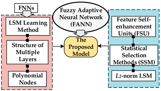
Figure 1.
Design overview of the proposed FANN.
The main contributions of the proposed FANN can be summarized as follows:
- (1)
- A design methodology incorporating the FSU to enhance the robustness and performance of the model. By preserving important features from raw data, the FANN maintains the physical significance of the original features, resulting in improved interpretability and readability.
- (2)
- Effective mitigation of overfitting by integrating the SSM and ℓ2-norm regularization learning techniques. The selected input subsets, derived from low-complexity raw data, and the regularization approach with penalty terms contribute to a more robust model.
- (3)
- Synergistic design: The FANN combines feature projection, clustering algorithms, and regularization techniques to address the limitations.
The paper is structured as follows: In Section 2, we present the details of the proposed FSU and the SSM. In addition, the theoretical explanation of the original model is supplemented. Comprehensive experimental results and experimental analysis are presented in Section 3 while conclusions, a few limitations, and future work that require more attention are drawn in Section 4.
2. Architecture of the Proposed Fuzzy Adaptive Neural Networks
2.1. Structure of FNNs and Its Polynomial-Based Neuron
In this paper, a polynomial-based neuron approach and FNN frame are used to construct the proposed architecture where each variable is partitioned individually. The if-then rules of fuzzy theory can divide individual input variables for each layer by the use of space partitioning. Therefore, fuzzy relations defined in the Cartesian product of the spaces of the input variables in the FNN. In conventional FNNs, neurons typically employ linear functions to compute their output. However, linear functions may inadequately capture the nonlinear relationships between input variables in numerous instances. As a result, researchers have introduced polynomial neurons to enhance the nonlinear fitting capabilities [6,9]. Polynomial neurons facilitate the capturing of nonlinear relationships within the data, endowing the FNN model with robust fitting abilities. In comparison to linear neurons, polynomial neurons better approximate complex functional relationships, yielding improved prediction results for various practical applications. Additionally, polynomial neurons possess a relatively simple structure, enabling the fitting of diverse complexity functions by combining polynomials of different orders, which reduces the complexity and boosts computational efficiency. However, it is important to note that increasing polynomial orders may lead to overfitting [10,11].
The conventional FNN exhibits a flexible model size, which varies according to the specific variants employed. The general structure of FNN consists of four primary components, as depicted in Figure 2. Fundamentally, the FNN model comprises an aggregation of fuzzy ‘if-then’ rules, where the i-th rule can be represented as follows:
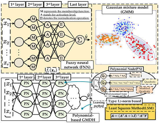
Figure 2.
General structures of FNNs and its structure of polynomial neuron.
In Figure 2, “M” represents the membership function, in which the parameters of the membership function were generated from the previous layer “A” is the activation level. The loss function of the FNN can be written as:
where n stands for the index of rules, is the label of the lth data pattern, is the vector for current input space, is the activation level, and is the conclusion part of the ith fuzzy rule. During the calculation of membership degrees, various membership functions can be employed, such as sigmoid, triangular, and others. In Equations (3) and (4), the sigmoid function serves as an example.
where and are the input vector and the random bias. In the consequent part of FNNs, to enhance the generalization of neurons, a series of conclusion parts (polynomial types) are considered, as summarized in Table 1. The coefficients of FNNs can be generated using the least squares error method. The objective function is expressed as follows:
where represents the model target output; is the activation level of the lth data pattern. To improve the adaptive properties of polynomial node to different scenarios, the polynomial function , shown in Table 1, contains not only a single constant but also linear and nonlinear combinations of input variables.

Table 1.
Types of Polynomial Functions and Their Expressions.
2.2. Statistical Selection Methods
The SSM improves the interpretability of the FANN model by retaining only features significantly related to the output. This enhances the model’s understandability and interpretability, promoting better results in practical applications. The SSM eliminates irrelevant or redundant information, improving the modeling accuracy and generalization capacity of the network. Furthermore, the SSM reduces the network’s computational complexity by removing unnecessary features and nodes, resulting in faster training and inference times. Overall, employing the SSM enhances the performance and efficiency of models under various conditions. Specifically, the SSM aims to elucidate the relationship between variables and the data’s underlying distribution, while regression in machine learning models this relationship to predict outcomes. Concurrently, statistical methods investigate the relationship between two variables and facilitate predictive modeling [12,13]. Due to their shared objectives, these techniques are complementary and interconnected. This paper presents two types of SMMs: correlation coefficient selection (CCS) and univariate linear regression tests (ULRTs). The chosen SMM types offer several benefits that contribute to the improved performance and robustness of the FANN model. First, they facilitate the integration of significant features into the network, promoting diversity among the neurons and ultimately improving the performance. Second, these SMM types are well suited to the FANN model’s architecture, enabling a seamless combination of different techniques for a more effective learning process. CCS and the ULRT are specifically designed to tackle regression problems. These methods excel at identifying and selecting the most relevant and significant features, which are crucial for enhancing the performance of the FANN in addressing regression tasks.
2.2.1. Details of Correlation Coefficient Selection
From the dual perspectives of machine learning and statistics, CCS is a prevalent feature selection technique employed to select the most pertinent features for model training. From a statistical point of view, the correlation coefficient gauges the linear association between two variables. CCS evaluates the correlation of each feature with the target variable, whereby features exhibiting high correlation coefficients are deemed critical to the model, while those with low coefficients are often deemed immaterial or duplicative. From a machine learning perspective, CCS is more suitable for regression models because it focuses on the relationship between the features and the target variable [14]. In a regression model, the goal is to predict a continuous target variable, and features that are highly correlated with the target variable are more likely to contribute to accurate predictions. Additionally, by selecting only the most relevant features, CCS can reduce the dimensionality of the input data, which can improve the performance and efficiency of the model. It ranges from −1 (perfectly negative correlation) to 1 (perfectly positive correlation) [15]. The formula is (given paired data consisting of m pairs):
where m is the size of data, and represent individual sample points indexed by ‘k’ and is the mean of sample and analogously for .
2.2.2. Introduction of the Univariate Linear Regression Tests
Utilizing univariate linear regression tests, which yield F-statistics and p-values, constitutes a crucial approach for feature selection in regression problems. This method involves assessing the impact of individual regressors sequentially across multiple variables. Moreover, the field of feature selection encompasses a diverse array of solutions, originating from various methodological perspectives. Furthermore, the primary benefits of the ULRT can be summarized as follows: First, ULRT-based feature selection emphasizes the computation of F-statistics (a statistical measure) for each variable independently, utilizing the magnitude of the F-value to ascertain the importance of features [14,16]. Second, in general, applying distinct models, such as regression and classification, to specific feature selection tasks can be challenging. However, the ULRT exhibits broad applicability to various problems in the machine learning domain, unrestricted by models or datasets. Lastly, this intuitive approach is easily replicable and modifiable, offering robust expressiveness in data analysis. Its exceptional statistical properties enable effective data interpretation. The subsequent hypotheses are commonly employed in the ULRT:
H0.
µ1 = µ2 = … = µk
H1.
At least one of the means is significantly distinct from the others.
The ULRT process can be broken down into the following steps:
- (1)
- Obtain the critical value (d.f.N and d.f.D) by computing the degrees of freedom. Specifically, the degrees of freedom for d.f.N are k − 1, where k represents the number of groups being compared, while the degrees of freedom for d.f.D are N − k and where N is the total sample size across all groups ;
- (2)
- Calculate the grand mean) , which is the mean of all values across all samples.
- (3)
- Compute the sum of squares between groups (), which is the sum of squared differences between the means of each sample and the grand mean, weighted by the sample sizes. Additionally, compute the sum of squares within groups (), which is the sum of squared differences between each observation and its sample mean. The function of () and () can be written as follows:where is the mean value of each variety and is the k-th variety and the l-th sample.
- (4)
- Obtain the F-value associated with the F-statistic (the value is SSB divided by SSW).
2.3. Description of a Feature Self-Enhancement Unit
In 2021, Zayed et al. proposed a hybrid adaptive neuro-fuzzy inference system integrated with an equilibrium optimizer algorithm. The equilibrium optimizer (EO) used in this study is employed as a new metaheuristic approach to enhance the prediction accuracy of the adaptive neuro-fuzzy inference system (ANFIS) [17]. Additionally, Sharafati et al. utilized optimization algorithms such as particle swarm optimization (PSO) and genetic algorithm (GA) to construct hybrid neuro-fuzzy models in the same year [18]. Their research investigated the sediment removal estimation of sediment ejectors using newly developed hybrid data-intelligence models. Inspired by these related works, we considered using the widely accepted gaussian mixture model in the proposed FANN. The gaussian mixture model is a probabilistic model widely employed in the fields of machine learning and statistics for clustering, density estimation, and pattern recognition. The gaussian mixture model operates under the assumption that the data are generated from a mixture of several Gaussian distributions with distinct means and covariances. The objective of the model is to identify these underlying Gaussian components and estimate their parameters [19,20]. The following probability density function exists for the Gaussian distribution of a one-dimensional random variable X:
where is the standard deviation and is the expected value of X, respectively. GMMs offer several advantages, such as their ability to model complex data distributions and the flexibility to capture different shapes and sizes of clusters.
The FSU is designed to improve the performance of machine learning models by concentrating on the most relevant and significant features within the data. Utilizing a combination of techniques, such as statistical methods and GMM algorithms, the FSU automatically adjusts and optimizes feature weights. The primary concept of the FSU is to emphasize the most critical and informative features in the dataset while minimizing the impact of noise and irrelevant information. This objective is achieved through the following steps:
[Step 1] Statistical methods: FSUs leverage statistical techniques, such as correlation analysis and feature ranking, to identify the most significant features that have a strong relationship with the target variable. This process helps in reducing the dimensionality of the input data and simplifying the model structure, thereby improving its interpretability.
[Step 2] The gaussian mixture model: By employing the GMM, the FSU can group similar data points or features together based on their patterns and relationships. This step aids in uncovering the underlying structure of the data and contributes to the identification of relevant feature subsets.
[Step 3] Feature weight optimization: The FSU automatically adjust and optimize feature weights based on their significance and contribution to performance of the proposed model. This process directs the attention of the FANN towards the most critical features, leading to enhanced predictive accuracy and generalization capabilities.
2.4. The Learning Method of the Proposed Model
Given that the degree of the polynomial significantly influences the complexity of neuron nodes, the standard least squares method (LSM) may yield unstable coefficients during the learning process. To tackle this challenge, a regularization technique has been incorporated into the conventional LSM, resulting in an extended least squares method. [21]. The main advantages of ℓ2-norm regularization can be summarized as follows: (1) ℓ2-norm regularization effectively manages model complexity by penalizing substantial weights, thereby reducing overfitting risks, particularly in high-dimensional scenarios with limited training samples. This approach fosters a balance between underfitting and overfitting, ultimately enhancing the model’s generalization capabilities; (2) in contrast to ℓ1-norm regularization (Lasso), which promotes sparsity by nullifying certain features, ℓ2-norm regularization results in a more equitable weight distribution across all features. This attribute is beneficial when multicollinearity is present, as it allocates the influence of correlated features more evenly, diminishing dependence on a single predictor; (3) ℓ2-norm regularization bolsters numerical stability during the learning process by rendering the loss function strongly convex, ensuring the existence of a unique global minimum and a well-posed optimization problem. Furthermore, the regularization technique can be employed in the learning method without impacting its computational performance, while the variance factor also serves to reduce bias [22,23]. Additionally, ℓ2-norm LSM can help to simplify the interpretation of the model by reducing the number of variables used in the final model. The combination of statistical selection methods with ℓ2-norm regularization can lead to a more balanced model by simultaneously reducing the complexity of the model and promoting the selection of relevant features. Additionally, the ℓ2-norm regularization can help to prevent overfitting by introducing a penalty term to the loss function, which encourages smaller weights and a smoother decision boundary. The loss function of ℓ2-norm LSM is summarized as follows:
where variable represents the ℓ2 regularization parameter, represents the coefficients of the polynomial function, and n represents the number of coefficients.
2.5. The Framework of the Proposed FANN
In this paper, a polynomial-based hybrid fuzzy neural network was proposed through statistics-based neuron selection and feature self-enhancement. The entire procedure of the proposed model is illustrated in Figure 3, while the topologies of the model are depicted in Figure 4. The FANN is a synergy of FNN, polynomial neuron, and the proposed techniques (a feature self-enhancement unit or FSU, and the statistics-based neuron selection method or SSM). This combination retains crucial information from raw data and demonstrates outstanding performance. The SSM in regression and FNN are based on multiparameter regression models. The main concept of the FANN can be summarized as follows: The output (selected subset) of the SSM is continually incorporated into each hidden layer after fuzzy transformation as an additional new input for each layer. Consequently, the inputs for the nth layer comprise the selected outputs with the best predictive ability from the (n − 1)th layer, along with additional inputs generated by the SSM in regression. The SSM utilized in the proposed FANN design is applied in two aspects: the generation of extra nodes (ENs) and the evaluation of network nodes. Figure 4 illustrates the two application parts of the SSM and the topology of the proposed FANN. Nodes in each layer of the FANN comprise a mixture of polynomial-based fuzzy neuron (pFN) and EN, with the generation of new nodes in each layer determined by SSM evaluation. In the current study, the initial layer of the proposed model incorporates the FSU, effectively reducing the influx of superfluous, redundant data into the model. To minimize computational expenses and overfitting, the second layer is constructed with fuzzy neurons, while the third layer and any subsequent layers consist of optional polynomial nodes. Based on this architecture, the crucial features identified by the SSM are integrated into the training process for the second layer and all higher layers, preserving the significant attributes provided by the original dataset.
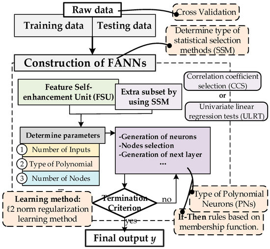
Figure 3.
Overall design flowchart of the FANN.
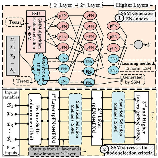
Figure 4.
Topology of the FANN structure based on different neurons.
3. Experimental Studies
3.1. Experimental Measurement Standard and Model Parameter Options
For the experiment part, we conducted the simulations on a computer equipped with an Intel (Santa Clara, CA, USA) Core i7-9700K CPU @ 3.60 GHz, 16 GB RAM, and an NVIDIA (Santa Clara, CA, USA) GeForce RTX 2080 GPU. The operating system used was Windows 10 (Microsoft, Redmond, WA, USA). The application platform for our experiments was the MATLAB, which provided an interactive environment for the implementation, testing, and visualization of our proposed model and the comparative experiments.
The outcomes of the suggested model are delineated by employing the mean square error (MSE) and the root mean square error (RMSE) metrics, which are expressed in terms of their respective means and standard deviations (STD) [24,25]. MSE and RMSE balance model bias (systematic errors) and variance (random errors). By minimizing these metrics, the model seeks an equilibrium between underfitting (high bias) and overfitting (high variance), crucial for effective generalization. The loss functions associated with RMSE and MSE can be characterized as follows:
where means the real output and denotes output of the neural network.
The assessment of the modeling performance for the proposed networks is con-ducted through the utilization of k-fold cross-validation. The complete dataset is partitioned into k segments, with k − 1 segments employed as the training set and the residual segment serving as the test set. For each dataset used in experiment part, we adopted the widely accepted 90–10 split, where 90% of the data was used for training, and the remaining 10% was used for testing. This division is a standard practice in machine learning research as it generally provides a sufficient amount of data for model training while still maintaining an adequate portion for model evaluation. To substantiate the importance of the proposed methodology, which encompasses the SSM, the FSU, ℓ2 regularization learning technique, and so forth, a collection of comparative experiments is devised in this paper. Concurrently, the two approaches (CCS and ULRT) encompassed by the SSM are incorporated into Proposed I and Proposed II, respectively. In addition, Table 2 and Table 3 show the main parameter details of the proposed model and give the specific values used in the experiment part. Table 4 shows the different conditions and main parameters of the two types of FANN models (FANN (I) and FANN (II)). Moreover, the parameter Type of SSM encompasses two sub-parameters: Threshold of SSM1 (TSSM1) and Threshold of SSM2 (TSSM2), which are utilized in the FSU module and the extra node generation part, respectively (refer to Figure 4).
Table 2.
Parameter Details.
Table 3.
Experimental Conditions between Two Proposed Models.
Table 4.
Details of the Dataset Used for the Experiment Part.
3.2. Publicly Available Datasets
The experimental investigations conducted in this study involve 16 datasets representing standard machine learning regression problems, sourced from the UCI Machine Learning Repository (https://archive.ics.uci.edu/ml/index.php (accessed on 15 January 2023)) [26]. To ensure the diversity of data in this experiment, the dataset features include
- -
- Low-dimensional datasets with limited size, e.g., MPG6, Basketball, and Cloud;
- -
- Medium-dimensional datasets with limited size, e.g., Thiazine and Pyrim;
- -
- Medium-dimensional datasets with moderately large size, e.g., Pumadyn, ParkinsonM, and ParkinsonT.
Throughout the experimentation, the 16 datasets obtained from the repository are utilized in a series of experiments, as referenced in Table 4. The selection of these numerical values was achieved through a trial-and-error process, which involved conducting multiple experiments to monitor the learning rate and assess convergence.
3.3. Experimental Analysis and Results
Table 5 and Table 6 present performance comparisons among various models, including Wake [27], other advanced FNN-based models [28,29], and the proposed FANN model.
Table 5.
Performance of the Proposed Model and Compare with Other Classical Machine Learning Models.
Table 6.
Performance of the Proposed Model and Compare with Other Advanced FNN-related Models.
In Table 5, by comparing the performance of the two FANN structures with six classical machine learning models from WEKA, we found that, out of datasets (1)~(12), the proposed FANN exhibited the best performance in 10 datasets. Furthermore, the proposed FANN (I) and FANN (II) of the two SSMs demonstrated exceptional competitive capacity.
In the discussion of the FANN for regression problems, it is essential to consider the advancements and alternative approaches in the field. Bayesian fuzzy clustering neural networks (BFCNNs) and regularized fuzzy neural networks (RFNNs) are two outstanding FNN-based network models in recent years [28,29]. The study of BFCNNs introduces a Bayesian fuzzy clustering approach to neural networks for addressing regression problems, further expanding the range of methodologies applicable to FANNs. The RFNN contributes to the field of fuzzy neural networks by incorporating regularization techniques to improve the generalization performance and reduce the complexity of the network. BFCNNs and RFNNs are two prominent FNN-based models in recent years, which boast excellent structure and performance. Comparing the performance of different models is a common practice in machine learning research, as it serves as a benchmark for measuring the success of new methods and helps researchers identify the best techniques for a given problem. Based on datasets (13)~(16), the performance and computation time of two other FNN-related models and two types of proposed structures are presented in Table 6 and Table 7, respectively. In 2021, Jeon et al. designed a LQR controller using fuzzy logic to account for the nonlinear and uncertain nature of wind turbines, which demonstrate its ability to improve the performance of large wind turbines in comparison to conventional control methods [30]. Additionally, these relevant works inspired us focusing on not increasing excessive model overhead. Therefore, the computational overhead of the FANN and its comparison model was provided in Table 6. Although the computation time of the target model is not the most competitive, the additional computation cost of the proposed model is acceptable. Figure 5 shows two example diagrams for each layer of highest weight neurons and its parent neurons. This indicates that the extra neurons selected by the SSM effectively participate in the construction of the subsequent highest weight neurons of each layer, which indicates the necessity of the extra neurons selected by the SMM in the FANN. Table 8 serves as a comparison between the proposed FANN model and the conventional FNN, examining the occurrence of overfitting in relation to the number of layers. In addition, Table 8 demonstrates whether overfitting occurs for different models across 12 datasets and the corresponding number of layers (with a maximum of 6 layers). This comparison underscores the effectiveness of the FANN model in mitigating overfitting compared to the conventional FNN model across various layers.
Table 7.
Comparison of Computation Time for Output Response in BFCNNs, RFNNs, and FANNs.
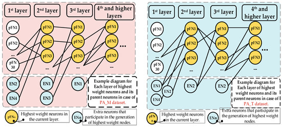
Figure 5.
Diagram for Each layer of highest weight neurons and its parent neurons (for the PA_M and PA_T).
Table 8.
Comparison of Overfitting Occurrence in Number of Layers between the Proposed FANN and Conventional FNN.
In Table 9 and Table 10, the performance of FANN (I) and FANN (II) is examined under various parameter values, showcasing the adaptability and robustness of the proposed model. These tables provide a comprehensive analysis of how different parameter settings affect the outcomes for the Ychat and PUMA datasets. The results highlight the effectiveness of the proposed FANN models and offer insights into the optimal parameter configurations for achieving the best performance in various scenarios. Furthermore, these tables allow readers to understand the sensitivity of the models to changes in parameter values and support the selection of appropriate parameter settings for future applications.
Table 9.
Comparison of Regression Results for Two Variants of FANNs with Different Parameter Settings (for the Ychat dataset).
Table 10.
Comparison of Regression Results for Two Variants of FANNs with Different Parameter Settings (for the PUMA dataset).
The FANN model outperformed the comparative models in 81.25% of the datasets. Although the computational cost for the BAS and CLO datasets increased by 7.82 s and 1.23 s, respectively, the corresponding performance improvement reached 6.8 and 4.4%. Notably, the CLE dataset exhibited not only a reduced computation time by 2.78 s but also an enhanced performance by 12.8%.
4. Conclusions
In this study, we have developed the proposed model, which is founded on two structures of the FANN model. The primary enhancements of the proposed methods stem from the integration of the SSM and the FSU with the conventional FNN and its polynomial neuron structure, yielding commendable performance. By integrating these techniques, the FANN model effectively reduces computational complexity, enhances interpretability, and mitigates overfitting. The synergistic combination of multiple technologies within the FANN architecture leads to improved performance, accuracy, and generalization capabilities. While the proposed FANN has shown promising results, there are still some limitations and opportunities for future research. The performance of the proposed model may be affected when dealing with large-scale datasets. Additionally, there might be other feature techniques that could further enhance the performance. Consequently, potential avenues for future research include two primary directions: (1) exploring techniques to improve the scalability and computational efficiency, such as parallel processing or more efficient optimization algorithms; and (2) investigating advanced methods to augment features.
Author Contributions
Conceptualization, Z.W. and Z.F.; methodology, Z.W.; software, Z.W.; validation, Z.W.; formal analysis, Z.W.; investigation, Z.W.; resources, Z.W.; data curation, Z.W.; writing—original draft preparation, Z.W.; writing—review and editing, Z.W.; visualization, Z.W.; supervision, Z.F.; funding acquisition, Z.F. All authors have read and agreed to the published version of the manuscript.
Funding
This work was funded by the National Research Foundation of Korea (NRF) grant funded by the Korea Government (MIST) (NRF-2021R1A2C1095739).
Informed Consent Statement
This article does not contain any studies with human participants or animal performed by any of the authors.
Data Availability Statement
The data presented in this study are available on request from the corresponding author.
Acknowledgments
We express our sincere appreciation to Kun Zhou, Hao Huang, Shuangrong Liu and TuTu Zhang for their constructive feedback and insightful discussions throughout the course of this work. This work was supported by the National Research Foundation of Korea (NRF) grant funded by the Korea Government (MIST) (NRF-2021R1A2C1095739).
Conflicts of Interest
The authors declare no conflict of interest.
References
- Engelbrecht, A.P. Computational Intelligence: An Introduction, 2nd ed.; John Wiley & Sons: Hoboken, NJ, USA, 2007. [Google Scholar]
- Agarwal, R.; Dhar, V. Big data, data science, and analytics: The opportunity and challenge for IS research. Inf. Syst. Res. 2014, 25, 443–448. [Google Scholar] [CrossRef]
- Siddiqi, M.A.; Pak, W. Optimizing filter-based feature selection method flow for intrusion detection system. Electronics 2020, 9, 2114. [Google Scholar] [CrossRef]
- Farlow, S.J. Self-Organizing Methods in Modeling: GMDH Type Algorithms; CRC Press: Boca Raton, FL, USA, 2020. [Google Scholar]
- Buckley, J.J.; Hayashi, Y. Fuzzy neural networks: A survey. Fuzzy Sets Syst. 1994, 66, 1–13. [Google Scholar] [CrossRef]
- Gupta, M.; Rao, D. On the principles of fuzzy neural networks. Fuzzy Sets Syst. 1994, 61, 1–18. [Google Scholar] [CrossRef]
- Chen, C.P.; Liu, Y.-J.; Wen, G.-X. Fuzzy neural network-based adaptive control for a class of uncertain nonlinear stochastic systems. IEEE Trans. Cybern. 2013, 44, 583–593. [Google Scholar] [CrossRef] [PubMed]
- Zhang, B.; Gong, X.; Wang, J.; Tang, F.; Zhang, K.; Wu, W. Nonstationary fuzzy neural network based on FCMnet clustering and a modified CG method with Armijo-type rule. Inf. Sci. 2022, 608, 313–338. [Google Scholar] [CrossRef]
- Han, H.; Qiao, J. A self-organizing fuzzy neural network based on a growing-and-pruning algorithm. IEEE Trans. Fuzzy Syst. 2010, 18, 1129–1143. [Google Scholar] [CrossRef]
- Zarandi, M.F.; Türksen, I.B.; Sobhani, J.; Ramezanianpour, A.A. Fuzzy polynomial neural networks for approximation of the compressive strength of concrete. Appl. Soft Comput. J. 2008, 8, 488–498. [Google Scholar] [CrossRef]
- Janczak, A. Identification of Nonlinear Systems Using Neural Networks and Polynomial Models: A Block-Oriented Approach; Springer Science & Business: Berlin/Heidelberg, Germany, 2004. [Google Scholar]
- Chandrashekar, G.; Sahin, F. A survey on feature selection methods. Comput. Electr. Eng. 2014, 40, 16–28. [Google Scholar] [CrossRef]
- Solorio-Fernández, S.; Carrasco-Ochoa, J.A.; Martínez-Trinidad, J.F. A review of unsupervised feature selection methods. Artif. Intell. Rev. 2020, 53, 907–948. [Google Scholar] [CrossRef]
- Zhou, H.; Wang, X.; Zhu, R. Feature selection based on mutual information with correlation coefficient. Appl. Intell. 2022, 52, 5457–5474. [Google Scholar] [CrossRef]
- Gonon, L.; Grigoryeva, L.; Ortega, J.P. Approximation bounds for random neural networks and reservoir systems. Ann. Appl. Probab. 2023, 33, 28–69. [Google Scholar] [CrossRef]
- Kokaly, R.F.; Clark, R.N. Spectroscopic determination of leaf biochemistry using band-depth analysis of absorption features and stepwise multiple linear regression. Remote Sens. Environ. 1999, 67, 267–287. [Google Scholar] [CrossRef]
- Zayed, M.E.; Zhao, J.; Li, W.; Elsheikh, A.H.; Abd Elaziz, M. A hybrid adaptive neuro-fuzzy inference system integrated with equilibrium optimizer algorithm for predicting the energetic performance of solar dish collector. Energy 2021, 235, 121289. [Google Scholar] [CrossRef]
- Sharafati, A.; Haghbin, M.; Tiwari, N.K.; Bhagat, S.K.; Al-Ansari, N.; Chau, K.W.; Yaseen, Z.M. Performance evaluation of sediment ejector efficiency using hybrid neuro-fuzzy models. Eng. Appl. Comput. Fluid Mech. 2021, 15, 627–643. [Google Scholar] [CrossRef]
- Pérez-del-Pulgar, C.J.; Smisek, J.; Rivas-Blanco, I.; Schiele, A.; Muñoz, V.F. Using Gaussian mixture models for gesture recognition during haptically guided telemanipulation. Electronics 2019, 8, 772. [Google Scholar] [CrossRef]
- Yuan, Y.; Liu, J.; Chi, W.; Chen, G.; Sun, L. A Gaussian Mixture Model Based Fast Motion Planning Method Through Online Environmental Feature Learning. IEEE Trans. Ind. Electron. 2022, 70, 3955–3965. [Google Scholar] [CrossRef]
- Caponnetto, A.; De Vito, E. Optimal rates for the regularized least-squares algorithm. Found. Comput. Math. 2007, 7, 331–368. [Google Scholar] [CrossRef]
- Tibshirani, R. Regression shrinkage and selection via the lasso. J. R. Stat. Soc. B Stat. Methodol. 1996, 58, 267–288. [Google Scholar] [CrossRef]
- de Matos, J.; Ataky, S.T.M.; de Souza Britto, A., Jr.; Soares de Oliveira, L.E.; Lameiras Koerich, A. Machine learning methods for histopathological image analysis: A review. Electronics 2021, 10, 562. [Google Scholar] [CrossRef]
- Willmott, C.J.; Matsuura, K. Advantages of the mean absolute error (MAE) over the root mean square error (RMSE) in assessing average model performance. Clim. Res. 2005, 30, 79–82. [Google Scholar] [CrossRef]
- Chai, T.; Draxler, R. Root mean square error (RMSE) or mean absolute error (MAE)?–Arguments against avoiding RMSE in the literature. Geosci. Model Dev. 2014, 7, 1247–1250. [Google Scholar] [CrossRef]
- UCI Machine Learning Repository. Available online: https://archive.ics.uci.edu/ml/index.php (accessed on 15 January 2023).
- Hall, M.; Frank, E.; Holmes, G.; Pfahringer, B.; Reutemann, P.; Witten, I.H. The WEKA data mining software: An update. ACM SIGKDD Explor. Newsl. 2009, 11, 10–18. [Google Scholar] [CrossRef]
- Souza, P.V.D.C.; Guimares, A.J.; Rezende, T.S.; Araujo, V.S.; Araujo, V.J.S.; Batista, L.O. Bayesian fuzzy clustering neural network for regression problems. In Proceedings of the IEEE International Conference on Systems, Man and Cybernetics, Bari, Italy, 6–9 October 2019; pp. 1492–1499. [Google Scholar]
- de Campos Souza, P.V.; Guimaraes, A.J.; Araújo, V.S.; Rezende, T.S.; Araújo, V.J.S. Fuzzy neural networks based on fuzzy logic neurons regularized by resampling techniques and regularization theory for regression problems. Intel. Artif. 2018, 21, 114–133. [Google Scholar] [CrossRef]
- Jeon, T.; Paek, I. Design and verification of the LQR controller based on fuzzy logic for large wind turbine. Energies 2021, 14, 230. [Google Scholar] [CrossRef]
Disclaimer/Publisher’s Note: The statements, opinions and data contained in all publications are solely those of the individual author(s) and contributor(s) and not of MDPI and/or the editor(s). MDPI and/or the editor(s) disclaim responsibility for any injury to people or property resulting from any ideas, methods, instructions or products referred to in the content. |
© 2023 by the authors. Licensee MDPI, Basel, Switzerland. This article is an open access article distributed under the terms and conditions of the Creative Commons Attribution (CC BY) license (https://creativecommons.org/licenses/by/4.0/).