Dynamic Models with Sigmoid Corrections to Generation of an Achievable 4D-Trajectory for a UAV and Estimating Wind Disturbances

Abstract

For an unmanned aerial vehicle (UAV) of an aircraft type, the problems of planning achievable trajectories as well as robust control under wind disturbances are considered. A computationally simple method for compiling a primary non-smooth 4D trajectory is proposed. Its segments connect the given waypoints and determine the desired average velocity in various sections. Instead of time-consuming methods of analytical smoothing of broken path joints using polynomials, a tracking differentiator with S-shaped smooth and limited sigmoid corrective actions is developed. This virtual dynamic model provides natural smoothing of the primary trajectory considering the design constraints on the velocity, acceleration, and thrust of the UAV. The tracking differentiator variables create an achievable trajectory and are used to synthesize the UAV tracking system. To compensate for the action of wind disturbances on the UAV, a disturbance observer is developed. It is a replica of the equations of the control plant model, which are directly affected by external uncontrolled disturbances. These algorithms also use sigmoid corrections. Unlike standard disturbances observers, this approach does not require the development of a dynamic model of external disturbances and does not assume their smoothness. The effectiveness of the developed algorithms was confirmed by numerical simulation.

1. Introduction

Motion planning is an independent task in the problems of automatic control of autonomous mobile robots. Currently, there are many path-planning methods for unmanned mobile robots on planes and in space within different approaches [1,2,3,4,5]. Each has benefits and drawbacks and recommendations for application, depending on the set of factors considered and relevant. These factors include the mission of the robot or group of robots; configuration and features of the workspace; obstacles; sensing capabilities and design limitations of the robot that determine its maneuverability; safety requirements, etc. A combination of different planning methods typically provides the best performance [6,7,8,9]. However, more accurate and optimal solutions, that consider many factors require constant correction during robot operation and are often accompanied by cumbersome geometric calculations and high computational costs. Therefore, it is not always possible to implement them in real time on an onboard computer. In particular, planning the motion of a robot in a dynamic environment, and avoiding collisions with several dynamic obstacles, is still an unsolved problem due to the lack of time to generate a safe trajectory [10,11].

In this paper, we do not consider the problem of obstacle avoidance. We investigate the problem of planning smooth and achievable trajectories with continuous curvature in structured environments. This problem is relevant for designing safe automatic control systems for wheeled robots and airplane-type aircraft. We cannot send abrupt command signals to a mechanical control plant. The vehicle cannot change direction instantly; therefore, if it changes course abruptly, it will not make the turn, drift out of its path, and cause an accident. In this paper, we present original methods for planning the achievable trajectory and controlling the center of mass of an unmanned aerial vehicle (UAV). We consider UAVs that deliver cargo to a target location or perform aerial photography of a controlled area (e.g., for crop monitoring in agriculture, environmental monitoring, etc.) under conditions of wind disturbances.

Researchers usually use interpolation algorithms and polynomial approximations to construct smooth trajectories. The standard solution consists of two steps. In the first stage, a set of waypoints is defined. Researchers connect them by segments or step functions and obtain a first approximation of the robot’s path in the workspace $D$ [7]. To create a primitive path for the center of mass of the UAV, a 3D polyline is set using waypoints $(x, y, z)\in D\subset R^3$. To create a primary trajectory, the reference points $(x, y, z, t)\in R^4$ for the 4D curve are set. The second stage uses various geometric constructions or Computer Aided Geometric Design (CAGD) techniques for a given set of control waypoints. This set is used to smooth out the primary polyline in the joints and obtain an achievable path or trajectory. A trajectory, which researchers usually define in parametric form, is achievable for a mechanical plant if it is a smooth function of class $C^2$ or higher. It must also have continuous curvature, satisfying the design constraints on the velocity and acceleration of the mobile robot.

For smoothing the reference path analytically, a basic set of control waypoints is defined at the joints of the polyline in each section. To connect them, the researchers use circle fragments or cubic curves, whose parameters they calculate from the coordinates of the four control waypoints. They also often use B’ezier Curves and Bernstein polynomials, which provide continuous curvature in the presence of seven control waypoints. Efficient methods for obtaining smooth curves are polynomial splines [12], clothoids [13], generalized Cornu spirals [14], etc. Cubic B-splines [2,10,15] are the most widely used at present. Their factors are calculated from the coordinates of the five control waypoints, which ensure that the curvature of the path changes smoothly. To obtain smooth curves of complex shapes, we need to increase the number of control waypoints in each joint of the polyline, which will lead to more complex calculations and increase the counting time of the algorithm. An additional problem in smoothing reference curves of complex shapes is the smooth joining of spline segments approximating neighboring joints in so-called knots. In addition, the problem of satisfying design constraints on the velocity, acceleration, and thrust of the UAV requires additional verification and algorithms. Thus, computational algorithms designed for analytical smoothing of multinode reference polylines, which solve all these problems, can be quite cumbersome and inefficient when implemented in online mode.

Our goal is to simplify and automate as much as possible the computational aspect of planning achievable 4D trajectories. This requires defining a smooth spatial path for the UAV’s center of mass as well as the desired velocity in flight mode at different locations, considering design constraints on the velocity, acceleration, and thrust of the UAV. Instead of the above methods of analytical smoothing of the reference trajectory, we propose dynamic smoothing that does not require complex geometric calculations, an exact analytical description of the trajectory segments, and the calculation of the appropriate polynomial factors. In our previous papers [16,17], we designed a dynamic generator of admissible trajectories for aircraft-type UAVs. This is an autonomous sixth-order dynamic virtual model, which is constructed as a replica of the input-output canonical model describing the motion of the UAV’s center of mass. Its corrective actions are analogous to the control actions of the control plant. A generator with closed-loop feedback is a tracking differentiator [18,19]. Its output variables track, with some accuracy, piecewise continuous signals from an autonomous source in real time.

The principle of the tracking differentiator is quite obvious. The dynamic object automatically provides a smooth output function whenever a spike is detected. We have developed a method that additionally ensures that controlled signals are restricted within specified ranges for tracking non-smooth signals. The main features of the designed algorithms are: (i) the use of S-shaped smooth and bounded sigmoid corrective actions [20,21]; (ii) the procedure of setting its gains considering the velocity and acceleration limitations of a particular UAV. In this way, the generator variables generate a naturally smooth trajectory and provide component-by-component information about its first and second derivatives. These signals are achievable reference actions and are used in the UAV control system.

The following results are the main contributions of this paper, in which we use and develop the approach described above:

• A simple method of composing a primary piecewise continuous 4D trajectory in the form of a polyline, which defines in first approximation the path of the UAV passing through the given reference waypoints $(x, y, z)\in D\subset R^3$. We can use the fourth coordinate $(x, y, z, t)$ to set the average desired velocity of flight in different parts of the trajectory, not exceeding the maximum velocity of a particular vehicle. The novelty of the proposed approach consists in formalizing the requirements for a primitive trajectory. It is easy to ensure that they are satisfied at the design stage, but there is no opportunity for online correction;
• A ninth-order tracking differentiator with sigmoidal corrective actions to smooth the reference trajectory and generate allowable reference actions for UAV position, velocity, and acceleration component by component. We developed a decomposition procedure to set up its gains considering the design constraints on UAV state variables. It is also shown that unlike the sixth-order dynamic generator [16,17], in this case, we can additionally ensure that the constraints on the third and fourth derivatives are satisfied, obtain a smoother signal for the second derivative, and reduce the algorithm’s counting time. The novelty of the proposed approach lies in the fact that the tracking differentiator generates smooth signals and their derivatives of the required order (which is quite sufficient for the design of standard tracking systems) with automatic implementation of design constraints. The above traditional methods provide an analytical description of the reference actions but do not have full-fledged mechanisms to provide design constraints and require additional control;
• A combined control law that ensures that the UAV’s center of mass tracks a smoothed trajectory and is invariant to external uncontrollable disturbances by compensating them. A minimum-dimensional dynamic observer with sigmoidal corrective actions has also been developed, which estimates external disturbances by their effect on the control plant. Unlike known disturbance observers, the designed approach does not require a dynamic model of external disturbances and can estimate non-smooth disturbances with any given accuracy. The novelty of the proposed approach lies in the fact that in the design process, both the observation errors and their derivatives are stabilized. This makes it possible not to increase the dynamic order of the observer and to use its correcting actions instead of the observer’s variables for disturbance recovery.

Another problem that is investigated in this paper is invariance to wind disturbances. It is assumed that the flight is in normal flight mode and the wind strength does not exceed the acceptable norms (i.e., moderate wind not exceeding 4 on the Beaufort scale). However, its influence can interfere with the execution of a flight mission and the tracking of a given path. Therefore, many researchers have devoted their papers to the problem of controlling aircraft under windy conditions. For example, in early studies, researchers considered optimal program control methods [22]. For their implementation, the wind velocity field is assumed to be known, but it is difficult to obtain accurate information about the changing wind velocity field. Within the framework of differential game theory, researchers use the grid method [23], but its implementation requires complex calculations in seven dimensions on a supercomputer system.

Researchers in various applications have considered Lipschitz systems with uncertain input [24,25]. They also applied methods of adaptive control and integrator backstepping using barrier functions [26,27,28] by which they could inhibit external disturbances knowing only their maximum modulo values. However, these methods are implementable under the assumption that external disturbances are smooth. The same assumption of smoothness of uncertain functions has been made in papers where disturbance observers are used to compensate for uncertainties. In standard approaches, it is first necessary to construct a dynamical model simulating external actions [29,30,31]. This is possible only for a narrow class of disturbances. In other cases, researchers apply sliding mode observers of various types [32,33,34]. However, it always leads to an additional increase in the dynamical order of the controller and increases the counting time of the control signal.

In this paper, we applied a sigmoid-corrected dynamic disturbance observer (this is the smooth analog of the sign function) to estimate the external disturbances. This observer replicates the equations of the mathematical model of the control plant directly affected by external disturbances [35,36,37]. It allows us to estimate the external disturbances with any given accuracy by applying correcting actions of the observer. This approach does not require the use of a dynamic disturbance generator and allows us to extend the class of admissible disturbances to include bounded smooth and non-smooth measurable functions.

The simultaneous use of a tracking differentiator and a disturbance observer for dynamic feedback design will allow us to implement a simple and efficient combined control law with a linear stabilizing component and provide a reliable and safe tracking system for the UAV. We consider the problem in the deterministic formulation, and we do not consider the problems of noise research and filtering.

The paper has the following structure. In Section 2, we describe the model of the control plant, namely, the sixth-order equations of motion of the UAV center of mass. Within the block approach [21,38], we designed a basic combined control law with compensation for the impact of wind uncontrollable disturbances, which ensures tracking of a given admissible trajectory. We also formulated problem statements for the information support of the tracking system and give the main results in Section 3. In Section 3.1, we designed a method for generating a reference non-smooth 4D trajectory passing through the given waypoints and obtained the given primary post-component actions for all spatial coordinates, setting the desired flight velocity for the different sections of the path. In Section 3.2, we present a method for dynamically smoothing a primitive trajectory using a ninth-order tracking differentiator. In Section 3.3, we design a third-order sigmoid-corrected dynamic external disturbance observer. In Section 4, we present numerical simulation results confirming the effectiveness of the designed algorithms.

2. Problem Definition

Let us consider a model of the spatial motion of the center of mass of an aircraft-type UAV in flight mode [38,39]

$$\begin{array}{l}\dot{L}=V\cos \theta \cos \Psi , \dot{H}=V\sin \theta , \dot{Z}=-V\cos \theta \sin \Psi ;\\ \dot{V}=(u_1-\sin \theta )g+f_1(t), \dot{\theta }=\frac{(u_2-\cos \theta )g+f_2(t)}{V}, \dot{\Psi }=-\frac{g{u}_3+f_3(t)}{V\cos \theta },\end{array}$$

(1)

where ${(L, H, Z)}^{\mathrm{T}}\in D\subset R^3$ is the vector of output (controllable) variables, these spatial variables determine the position of the center of mass of the UAV in the trajectory coordinate system $D$: $L$ is the longitudinal flight range, $H$ is the flight altitude, $Z$ is the lateral deviation; $V$ is the real ground velocity; $\theta$ is the angle of inclination of the flight path to the horizon; $\Psi$ is the flight path angle. We assume that all of the above state variables are measured and that there is no noise interference, $V>0,$ $\left|\theta (t)\right|<\pi /2,$ $\left|\Psi (t)\right|<\pi /2,$ $t\ge 0$. Other notations used in the system (1): $g=9.81$ $[\mathrm{m}/{\mathrm{s}}^2]$ is the gravitational acceleration; $u={(u_1, u_2, u_3)}^{\mathrm{T}}$ are control actions (overload vector); $f={(f_1, f_2, f_3)}^{\mathrm{T}}$ are uncontrollable moments and forces, including wind forces. Assume that atmospheric conditions are suitable for the performance of the flight mission and that the maximum wind velocity at flight altitude does not exceed 2/3 of the maximum velocity of the UAV; $f(t)$ treated as a vector of external disturbances, its elements $f_j(t)$ are unknown bounded time functions

$$\Vert f(t)\Vert \le F, t\in [t_{\mathrm{start}}; t_{\mathrm{end}}],$$

smoothness requirements are not imposed on them, $F$ is a known positive constant, $[t_{\mathrm{start}}; t_{\mathrm{end}}]$ is flight time after altitude gain and before landing approach. Here and below, $\Vert \ast \Vert$ is $l_{\infty }$-norm of the vector, namely

$$F=\max \{F_1, F_2, F_3\}, \left|f_j(t)\right|\le F_j, j=1, 2, 3.$$

(2)

Let us introduce the following notation for output variables and their velocities:

$$\begin{array}{l}{y}_1={(y_{11}:=L, y_{12}:=H, y_{13}:=Z)}^{\mathrm{T}}\in Y_1\subseteq D\subset R^3, \\ {\dot{y}}_1=y_2={(y_{21}:=V\cos \theta \cos \Psi , y_{22}:=V\sin \theta , y_{23}:=-V\cos \theta \sin \Psi )}^{\mathrm{T}},\end{array}$$

(3)

where $Y_1$ is the acceptable working space in flight mode. Let us introduce system (1) in input-output form with canonical variables (3):

$$\begin{array}{l}{\dot{y}}_1=y_2, \\ {\dot{y}}_2=ag+B(\theta , \Psi )(gu+f(t)),\end{array}$$

(4)

where $a={\left(0; -1; 0\right)}^{\mathrm{T}};$

$$B=\left(\begin{array}{ccc}\cos \theta \cos \Psi & -\sin \theta \cos \Psi & \sin \Psi \\ \sin \theta & \cos \theta & 0\\ -\cos \theta \sin \Psi & \sin \theta \sin \Psi & \cos \Psi \end{array}\right), \det B\equiv 1, B^{-1}=B^{\mathrm{T}}.$$

In the notation of system (4), let us introduce design constraints on the state and control variables in flight mode:

$$\begin{array}{l}0<{\underset{\_}{V}}_0\le \Vert y_2(t)\Vert \le {\overline{V}}_0, \Vert {\dot{y}}_2(t)\Vert \le {\overline{V}}_1, \Vert {\ddot{y}}_2(t)\Vert \le {\overline{V}}_2, \\ \Vert u(t)\Vert \le U, t\in [t_{\mathrm{start}}; t_{\mathrm{end}}], F<gU, {\overline{V}}_0^2<gU<{\overline{V}}_1<{\overline{V}}_2.\end{array}$$

(5)

The upper estimate of the acceleration vector norm (and hence the velocity) is determined for the “worst case” where part of the control is spent on compensating external disturbances, namely:

$$\Vert {\dot{y}}_2\Vert =\Vert ag+B(\theta , \Psi )(gu+f)\Vert \le 3(gU-F)={\overline{V}}_1.$$

(6)

Let ${\chi }_1(t)={({\chi }_{11}(t), {\chi }_{12}(t), {\chi }_{13}(t))}^{\mathrm{T}}$ be a vector of the given actions for the output variables $y_1(t)$ of system (1). It sets in real time the desired spatial trajectory for the center of mass of the UAV when executing a specific work scenario at $t\in [t_{\mathrm{start}}; t_{\mathrm{end}}]$. Scenario execution time is bounded and depends on the energy source used [40]. Signals ${\chi }_{1j}(t)$ are sent to the control system in real time and set not only the spatial position but also the velocity and acceleration of the UAV in flight mode.

The given actions ${\chi }_{1j}(t), j=1, 2, 3$ are considered to be correctly defined and achievable if they satisfy the conditions below.

• The given path is in the working space, and the initial values of the reference actions and the controlled variables are sufficiently close:

  $$\begin{array}{l}{\chi }_1(t)\in Y_1, t\in [t_{\mathrm{start}}; t_{\mathrm{end}}];\\ \sqrt{{\displaystyle \sum _{j=1}^3{(y_{1j}(t_{\mathrm{start}})-{\chi }_{1j}(t_{\mathrm{start}}))}^2}}/{\underset{\_}{V}}_0<< t_{\mathrm{end}}-t_{\mathrm{start}}.\end{array}$$

  (7)
• The curvature of the path is continuous and the given actions are quite smooth

  $${\chi }_{1j}(t)\in C^3, i=1, 2, 3.$$

  (8)
• The values of the derivatives of the given actions do not exceed the design velocity and acceleration limits of UAV (5):

  $${\underset{\_}{V}}_0<\Vert {\dot{\chi }}_1(t)\Vert <{\overline{V}}_0, \Vert {\ddot{\chi }}_1(t)\Vert <{\overline{V}}_1, \Vert {\stackrel{⃛}{\chi }}_1(t)\Vert <{\overline{V}}_2, t\in [t_{\mathrm{start}}; t_{\mathrm{end}}].$$

  (9)

Assuming that conditions (7)–(9) are satisfied, we must design a feedback tracking system that ensures that the output variables of system (1) track the given signals and are invariant to external disturbances.

To design a tracking system, let us introduce the differential equation for the tracking error vector ${\xi }_1=y_1-{\chi }_1={({\xi }_{11}, {\xi }_{12}, {\xi }_{13})}^{\mathrm{T}}$ in the form of ${\dot{\xi }}_1=y_2-{\dot{\chi }}_1$. We can set the desired exponential tracking error stabilization rate with a linear local feedback $y_2={\dot{\chi }}_1-c_1{\xi }_1$, $c_1=\mathrm{const}>0,$ which we will control with a residual ${\xi }_2=y_2-{\dot{\chi }}_1+c_1{\xi }_1,$ ${\xi }_2={({\xi }_{21}, {\xi }_{22}, {\xi }_{23})}^{\mathrm{T}}.$ Then by virtue of (4), we obtain the following system for tracking errors

$$\begin{array}{l}{\dot{\xi }}_1=-c_1{\xi }_1+{\xi }_2, \\ {\dot{\xi }}_2=-c_1^2{\xi }_1+c_1{\xi }_2+ag-{\ddot{\chi }}_1+B(\theta , \Psi )(gu+f(t)).\end{array}$$

(10)

Suppose that the derivatives of the reference actions ${\dot{\chi }}_1(t), {\ddot{\chi }}_1(t)$ and external disturbances $f(t)$ are known time functions. Then we can compensate for their influence with a combined control and introduce a stabilizing linear component

$$\begin{array}{l}gu=-B^{\mathrm{T}}(\theta , \Psi )[(c_2+c_1){\xi }_2-c_1^2{\xi }_1-{\ddot{\chi }}_1+ag]-f(t)=\\ =-B^{\mathrm{T}}(\theta , \Psi )[c_1{c}_2(y_1-{\chi }_1)+(c_1+c_2)(y_2-{\dot{\chi }}_1)-{\ddot{\chi }}_1+ag]-f(t), \\ c_2=\mathrm{const}>0.\end{array}$$

(11)

In control law (11), the output variables $y_1(t)$ are measured and their velocities $y_2(t)$ are calculated based on the values $V(t), \theta (t), \Psi (t)$ from Equation (3).

A closed-loop virtual system (10) and (11) will take the following form

$$\begin{array}{l}{\dot{\xi }}_1=-c_1{\xi }_1+{\xi }_2, \\ {\dot{\xi }}_2=-c_2{\xi }_2.\end{array}$$

(12)

At $c_2\ge c_1$, the variables of system (12) will approach zero at a given rate

$$\Vert {\xi }_2(t)\Vert \underset{t\to +\infty }{=}O(\exp (-c_{2}t))\Rightarrow \Vert {\xi }_1(t)\Vert \underset{t\to +\infty }{=}O(\exp (-c_{1}t))\iff \underset{t\to +\infty }{\lim }{y}_1(t)={\chi }_1(t).$$

(13)

Thus, if the trajectory ${\chi }_1(t)$ is correctly specified and achievable, then in the closed-loop system (1), (11) the center of mass of the UAV (material point) will exponentially approach a given spatial curve and will move along it with a given velocity

$$\begin{array}{l}{\dot{y}}_1=y_2, \\ {\dot{y}}_2=-c_2{c}_1(y_1-{\chi }_1)-(c_2+c_1)(y_2-{\dot{\chi }}_1)+{\ddot{\chi }}_1=c_1^2{\xi }_1-(c_2+c_1){\xi }_2+{\ddot{\chi }}_1\Rightarrow \\ {\dot{y}}_2\underset{t\to +\infty }{=}{\ddot{\chi }}_1+(c_2+c_1)O(\exp (-c_{2}t))+c_1^{2}O(\exp (-c_{1}t)).\end{array}$$

The transients of the tracking errors depend on the proximity of the initial values and the gain factors considered

$$c_1{c}_2\Vert y_1(t_{\mathrm{start}})-{\chi }_1(t_{\mathrm{start}})\Vert +[(c_1+c_2)\Vert y_2(t_{\mathrm{start}})-{\dot{\chi }}_1(t_{\mathrm{start}})\Vert \le gU-F-\Vert {\ddot{\chi }}_1\Vert .$$

In this paper, we set the following problems related to the generation and estimation of external signals required for control design (11).

The first problem relates to planning the achievable trajectory over the given waypoints and the desired ground velocity in the various sections of the path (or, similarly, to providing the desired point-to-point flight time). Note that we do not consider the problem of precise movement from point to point in a given time, nor do we consider a full analytical description of the trajectory. Our task is first to check that the reference points are set correctly, to exclude forbidden maneuvers, and to design a primitive polyline connecting the corrected waypoints in analytical form as a function of time. Second, we must smooth the joints of the primitive polyline to satisfy the constraints (9) and provide the average desired velocity in the different sections. To design the control law (11), it is sufficient to obtain signals ${\chi }_1(t), {\dot{\chi }}_1(t), {\ddot{\chi }}_1(t),$ $t\in [t_{\mathrm{start}}; t_{\mathrm{end}}]$, that satisfy conditions (8) and (9). Thus, we obtain the reference trajectory in signal form instead of analytical form. The solution to these problems will be presented in Section 3.1 and Section 3.2, respectively.

Standard approaches use dynamic models that simulate external disturbances. We propose, however, to estimate $f(t)$ with a disturbance observer designed as a replica of the last three equations of system (1). The solution to this problem is presented in Section 3.3.

3. Theoretical Results

3.1. Primitive Trajectory Construction

Assume that a primary flight task plan is available for a particular UAV. This is a sequence of waypoints defined in a trajectory coordinate system in working space, considering the time

$$(L_i, H_i, Z_i, t_i), i=\overline{1, n}, (L_i, H_i, Z_i)\in Y_1, t_i<t_{i+1}, t_1=t_{\mathrm{start}}; t_n=t_{\mathrm{end}}.$$

(14)

With (14), we set the primary desired path and the average desired flight velocity for each section. Once again, note that we are not considering the problem of avoiding obstacles and avoiding collisions with moving obstacles here. We plan the trajectory for a postal vehicle or for a UAV taking video or photos of a monitored area after climbing to altitude and before landing approach in a calm atmosphere. Potential wind disturbances are not considered in these constructions. We will compensate for them in the tracking system with control (11).

First, we must verify that the waypoints are set correctly (14) and exclude forbidden maneuvers for aircraft-type UAVs. Let us list the items that require verification:

• Movements strictly “up and down”, i.e., $H_{i+1}\ne H_i$ and $L_i=L_{i+1}, Z_i=Z_{i+1}$, “in and out”, i.e., $L_i=L_{i+2}, H_i=H_{i+2}, Z_i=Z_{i+2}$ are forbidden;
• The acute angle between two neighboring sections connecting points $(L_i, H_i, Z_i)$ and $(L_{i+1}, H_{i+1}, Z_{i+1})$, $(L_{i+1}, H_{i+1}, Z_{i+1})$ and $(L_{i+1}, H_{i+1}, Z_{i+1})$ must not be smaller than the angle ${\varphi }_{\min }$ required to turn the UAV, namely:

  $$\arccos \left|\frac{(L_{i+1}-L_i)(L_{i+2}-L_{i+1})+(H_{i+1}-H_i)(H_{i+2}-H_{i+1})+(Z_{i+1}-Z_i)(Z_{i+2}-Z_{i+1})}{\sqrt{{(L_{i+1}-L_i)}^2+{(H_{i+1}-H_i)}^2+{(Z_{i+1}-Z_i)}^2}\cdot \sqrt{{(L_{i+2}-L_{i+1})}^2+{(H_{i+2}-H_{i+1})}^2+{(Z_{i+2}-Z_{i+1})}^2}}\right|\ge {\varphi }_{\min }, \forall i=\overline{1, n-2};$$
• The average ground velocity in each section must be allowable (9), i.e.,

  $${\underset{\_}{V}}_0<\frac{\sqrt{{(L_{i+1}-L_i)}^2+{(H_{i+1}-H_i)}^2+{(Z_{i+1}-Z_i)}^2}}{t_{i+1}-t_i}\le {\overline{X}}_2<{\overline{V}}_0, \forall i=\overline{1, n-1}.$$

  (15)

If these conditions are not satisfied for any pair or three neighboring waypoints, we need to make an appropriate correction so that the path stays in the workspace $Y_1$ and $t_n\le t_{\mathrm{end}}.$ If, after correction, $t_n>>t_{\mathrm{end}}$, then in a critical situation the flight task should be reduced so that the total time of the UAV in the air does not exceed the permissible value.

The corrected waypoints sequence is the basis for constructing a primitive continuous trajectory. It is set as a sequence of sections connecting neighboring waypoints

$$\frac{{\chi }_{11}-L_i}{L_{i+1}-L_i}=\frac{{\chi }_{12}-H_i}{H_{i+1}-H_i}=\frac{{\chi }_{13}-Z_i}{Z_{i+1}-Z_i}=\frac{t-t_i}{t_{i+1}-t_i}, t\in [t_i; t_{i+1}), i=\overline{1, n-1},$$

and defines the reference actions for each output variable $y_1={(y_{11}:=L, y_{12}:=H, y_{13}:=Z)}^{\mathrm{T}}$, respectively:

$$\{\begin{array}{l}{\chi }_{11}=\frac{(L_{i+1}-L_i)t+L_i{t}_{i+1}-L_{i+1}{t}_i}{t_{i+1}-t_i}, \\ {\chi }_{12}=\frac{(H_{i+1}-H_i)t+H_i{t}_{i+1}-H_{i+1}{t}_i}{t_{i+1}-t_i},\\ {\chi }_{13}=\frac{(Z_{i+1}-Z_i)t+Z_i{t}_{i+1}-Z_{i+1}{t}_i}{t_{i+1}-t_i}, t\in [t_i; t_{i+1}), i=\overline{1, n-1}.\end{array}$$

(16)

We will not apply analytical calculations to smooth the joints of the primitive trajectory (15) and (16). For natural smoothing, we use the dynamic model presented in the next subsection.

3.2. Tracking Differentiator Design

To design the tracking system (11), we need continuous signals that form an achievable trajectory (8) and their first and second derivatives that satisfy the given constraints (9). To smooth the primitive trajectory signals, we use a tracking dynamic differentiator with sigmoid correcting actions. Instead of following [16,17], in this paper, we will increase the order of the dynamic model used. It is to enable us to additionally enforce the design constraints on the third and fourth derivatives of the reference actions, as well as to reduce the outliers of the second derivative at special points (joints of polyline (16)).

Thus, we adopt the 9th-order dynamical canonical model

$${\dot{x}}_1=x_2, {\dot{x}}_2=x_3, {\dot{x}}_3=w$$

(17)

to generate an achievable trajectory and its first and second derivatives. Here, $w\in R^3$ is a vector of corrective actions. It is analogous to the third full derivative of the undisturbed model of the control plant (4), namely ${\ddot{y}}_2=g(\dot{B}u+B\dot{u}).$ We need to formulate the corrective actions in the form of feedback $w(x_1, x_2, x_3, {\chi }_1)$ so as to ensure that the output variables of the generator $x_1(t)\in R^3$ track continuous but non-smooth reference actions ${\chi }_1(t)\in Y_1\subset R^3$ (16) with a bounded derivative (15). At angular points ${\dot{\chi }}_1(t_i), i=\overline{2, n-1}$, the constraints are understood as one-sided. The accuracy of tracking, and hence obtaining smooth curves $x_1(t)$, depends on the constraints

$$\Vert x_2(t)\Vert \le X_2<{\overline{V}}_0, \Vert x_3(t)\Vert \le X_3<{\overline{V}}_1, \Vert {\dot{x}}_3(t)\Vert \le X_4<{\overline{V}}_2, t\in [t_{\mathrm{start}}; t_{\mathrm{end}}]$$

(18)

that we have to ensure in a closed-loop system (17). Then we can use the variables $x_1(t),$ $x_2(t)$ and $x_3(t)$ in control law (11) instead of ${\chi }_1(t),$ ${\dot{\chi }}_1(t),$ ${\ddot{\chi }}_1(t).$

To satisfy given constraints (18) in the design of corrective actions $w$ we will also, as in [16,17,20,21,38], use non-linear odd sigma-functions $\sigma (x)=-\mathrm{th}(-x/2), \sigma (-x)=-\sigma (x)$ in the local feedback. In order to set up the required features, we have introduced two scaling parameters $k, m=\mathrm{const}>0$ into the sigma function, namely

$$m\sigma (kx)=m\frac{1-\exp (-kx)}{1+\exp (-kx)},$$

where a gain $k$ determines the slope angle of the sigma function in a small neighborhood of zero. It plays the role of a high-gain factor in further constructions. Its value determines the accuracy of the tracking. A factor $m$ (amplitude) determines the stretching of the sigma function along the vertical axis and bounds its maximum modulo value. The derivative of the sigmoid function has a recursive form:

$$m{\sigma }^{\prime }(kx)=0.5mk(1-{\sigma }^2(kx)), 0<m{\sigma }^{\prime }(kx)\le 0.5mk, x\in R.$$

The results of initial research have shown that the type of logistic function used is not important for the following algorithms. The logistic function used is unimportant for the following algorithms. All of them provide good performance with the appropriate choice of mass-scaling factors. However, there are two reasons why we adopted the specified modification of the hyperbolic tangent composed of exponents for our design. Unlike other logistic functions, such as rational and root sigmoid, arctangent, etc., this function is, first, more useful for analyzing the stability of a closed-loop system, since its derivative is recursively expressed through the prime form. Second, its numerical realization is not problematic since the corresponding McLaren series converges on the entire numerical axis (unlike other mentioned transcendental functions whose McLaren series convergence area is bounded by a small numerical interval in the neighborhood of zero).

The points $\sigma (\pm 2.2)\approx \pm 0.8$ divide the sigma function into a conditionally linear function on the interval $[-2.2; 2.2]$ and a conditionally constant function on the intervals $(-\infty ; -2.2)$ and $(2.2; +\infty )$ [21]. Let $c>0$ be the abscissa modulus of the division point of the sigma function into a conditionally linear and a conditionally constant function. Its value is in the interval $c\in [1.3; 3]$ where $\pm 1.3$ are abscissa of the inflection points of the first derivative $\mathsf{\sigma }‴(\pm 1.3)=0,$ $\mathsf{\sigma }(\pm 1.3)\approx \pm 0.57;$ $\pm 3$ are abscissa of the vertices of the sigma function where its curvature reaches a maximum, $\mathsf{\sigma }(\pm 3)\approx \pm 0.9.$ For ease of calculation, we have adopted $c>2.2.$ Additional advantages of this choice are specified in [21].

The following estimates

$$\begin{array}{l}m\frac{0.8k}{2.2}\left|x\right|\approx 0.36mk\left|x\right|\le m\left|\sigma (kx)\right|\le 0.8m, k\left|x\right|\le 2.2; \\ 0.8m\le m\left|\sigma (kx)\right|<m, k\left|x\right|>2.2\end{array}$$

(19)

are valid in the specified zones.

Next, we demonstrate the developed procedure for the design of sigmoid corrective actions in system (17) consisting of three 3rd-order blocks. It is a logical continuation of the design procedure for the system consisting of two blocks [16,17], so here we give it without strict proof.

Let us introduce a tracking error $e_1=x_1-{\chi }_1\in R^3$. In the differential equation ${\dot{e}}_1=x_2-{\dot{\chi }}_1$, the derivative of the reference action ${\dot{\chi }}_1$ is treated as a bounded disturbance (15). To design system (4), we used linear local stabilizing feedback to the design system (10). In order to satisfy the given constraints (18) for the design of system (17), we introduce the sigmoid bounded stabilizing local feedbacks and appropriate residuals

$$\begin{array}{l}{e}_2=x_2+m_1\sigma (k_1{e}_1), e_3=x_3+m_2\sigma (k_2{e}_2), \\ e_i={(e_{i1}, e_{i2}, e_{i3})}^{\mathrm{T}}, i=2, 3,\end{array}$$

(20)

as well as a sigmoid corrective action

$$w=-m_3\sigma (k_3{e}_3),$$

(21)

where $m_i, k_i=\mathrm{const}>0, \sigma (k_i{e}_i)={(\sigma (k_i{e}_{i1}), \sigma (k_i{e}_{i2}), \sigma (k_i{e}_{i3}))}^{\mathrm{T}}, i=1, 2, 3.$

Let us redefine system (17) concerning tracking errors $e_1=x_1-{\chi }_1$ and residuals (20). Under (21), we obtain a closed-loop system

$$\begin{array}{l}{\dot{e}}_1=-m_1\sigma (k_1{e}_1)+e_2+{\eta }_1, \\ {\dot{e}}_2=-m_2\sigma (k_2{e}_2)+e_3+{\eta }_2,\\ {\dot{e}}_3=-m_3\sigma (k_3{e}_3)+{\eta }_3,\end{array}$$

(22)

where ${\eta }_i, i=1, 2, 3$ are treated as external bounded disturbances

$$\begin{array}{l}{\eta }_1=-{\dot{\chi }}_1, {\eta }_2=0.5m_1{k}_1{\Lambda }_1(x_2-{\dot{\chi }}_1), {\eta }_3=0.5m_2{k}_2{\Lambda }_2(x_3+0.5m_1{k}_1{\Lambda }_1(x_2-{\dot{\chi }}_1));\\ {\Lambda }_i=\mathrm{diag}({\Lambda }_{ij}), {\Lambda }_{ij}=1-{\sigma }^2(k_i{e}_{ij})), 0<{\Lambda }_{ij}\le 1, i=1, 2, j=1, 2, 3.\end{array}$$

(23)

Considering (15), (18), and (23), let us estimate the vector variables ${\eta }_i$:

$$\begin{array}{l}\Vert {\eta }_1\Vert \le {\overline{X}}_2, \Vert {\eta }_2\Vert \le 0.5m_1{k}_1(X_2+{\overline{X}}_2)=N_2,\\ \Vert {\eta }_3\Vert \le 0.5m_2{k}_2(X_3+0.5m_1{k}_1(X_2+{\overline{X}}_2))=0.5m_2{k}_2(X_3+N_2)=N_3.\end{array}$$

(24)

According to the block principle of control [20,21], we have to ensure that the state variables of the system (22) converge successively from bottom to top in the following neighborhoods of zero:

$$\Vert e_3\Vert \le 2.2/k_3\Rightarrow \Vert e_2\Vert \le 2.2/k_2\Rightarrow \Vert e_1\Vert \le 2.2/k_1\iff \Vert x_1-{\chi }_1\Vert \le 2.2/k_1.$$

(25)

Fulfilling the steady-state Equation (25) is the control goal in the tracking differentiator. We will ensure (25) by selecting the amplitudes $m_i$ based on the lower estimates obtained successively from the bottom up from sufficient conditions $e_i^{\mathrm{T}}{\dot{e}}_i<0, i=3, 2, 1$ considering (19) and (24):

$$\begin{array}{l}0.8m_3>N_3\Rightarrow e_3^{\mathrm{T}}{\dot{e}}_3\le \Vert e_3\Vert (N_3-0.8m_3)<0\Rightarrow \Vert e_3\Vert \le 2.2/k_3;\\ 0.8m_2>2.2/k_3+N_2\Rightarrow e_2^{\mathrm{T}}{\dot{e}}_2\le \Vert e_2\Vert (2.2/k_3+N_2-0.8m_2)<0\Rightarrow \Vert e_2\Vert \le 2.2/k_2;\\ 0.8m_1>2.2/k_2+{\overline{X}}_2\Rightarrow e_1^{\mathrm{T}}{\dot{e}}_1\le \Vert e_1\Vert (2.2/k_2+{\overline{X}}_2-0.8m_1)<0\Rightarrow \Vert e_1\Vert \le 2.2/k_1.\end{array}$$

(26)

To satisfy (18), let us bound from above the equations for the choice of $m_i$ by virtue of (20) and (21)

$$m_1\le X_2, m_2\le X_3,m_3\le X_4,$$

(27)

which will simultaneously bound the admissible values of $k_{1,2}$ and hence stabilization accuracy (25). Due to a priori assumptions (5), the system of dual inequalities (26), (27) is joint. The maximum admissible value $k_3$ depends on the available constraints on the fourth derivative of the output variables of system (4).

Thus, the closed-loop system (17), (21) has the form

$$\begin{array}{l}{\dot{x}}_1=x_2, {\dot{x}}_2=x_3, {\dot{x}}_3=-m_3\sigma (k_3{e}_3)=\\ =-m_3\sigma (k_3(x_3+m_2\sigma (k_2(x_2+m_1\sigma (k_1(x_1-{\chi }_1)))))).\end{array}$$

(28)

The scaling parameters of sigma functions satisfying (26) and (27) ensure that the output variables $x_1(t)$ of system (28) track the primitive trajectory (16) with some accuracy (25) and at the same time constrain the state variables considering (9). The dynamic model (28) naturally smooths the signals ${\chi }_1(t)$ at its input, so that the output generates an achievable trajectory $x_1(t)$ for the UAV’s center of mass. At the same time, the signals $x_2(t)$ and $x_3(t)$ provide the values of its first and second derivatives and are also used in the control law (11) instead of ${\dot{\chi }}_1(t)$ and ${\ddot{\chi }}_1(t)$ and do not lead to unacceptable overloads.

Note that the developed methods of design of sigmoid corrective actions fundamentally differ from the way of using sigmoid functions in the problems of neural network control. There, the regulator parameters are adjusted according to the known learning sample, in the formation of which, it is required to provide all possible modifications of the regulated process. In this paper, we use the sigma functions directly in the feedback loop of the tracking differentiator as corrective action. The scaling factors are assigned at the design stage based on equations that consider the “worst case” (24), (26) disturbances (23). During the control process in the virtual system (22), the sigmoid corrective actions converge to the disturbances in a finite time and repeat their shape with a specified accuracy. This automatically implements the disturbance compensation and residual stabilization mechanisms (25). As can be seen from Equation (20), the variables of the tracking differentiator $x_2, x_3$ “track” smooth and bounded sigmoid functions during the stabilization of the residuals $e_2, e_3$, thus ensuring (8). The fulfillment of Equation (27) ensures the specified constraints (5), (18). The necessary conditions (7), (9), which must be satisfied by an achievable trajectory, are ensured by composing a primitive trajectory (Section 3.1).

In contrast to the second-order tracking differentiator [16,17], where the second derivative signals are taken from the integrator input and directly contain ${\chi }_1(t)$, in system (28), we obtain ${\ddot{x}}_1(t)=x_3(t)$ from the integrator output. This provides additional filtering of ${\chi }_1(t)$ and smaller outliers of $x_3(t)$ at special points.

The calculation with the smoothing dynamic model (28) can be performed both offline and online. In the planning phase, we can simulate system (28) repeatedly in accelerated time and introduce the necessary corrections. We can also use algorithms (28) to treat a reference signal with additive noise [17] entering the UAV information and control system from an autonomous source in real time.

3.3. Disturbances Observer Design

In this subsection, we presented a method for designing a disturbance observer. This is a dynamic model that is implemented in the UAV real-time information and control system. It provides current estimates of external disturbances by their influence on the control plant. In contrast to known approaches, we can estimate with any given accuracy both smooth and non-smooth external disturbances, assuming that they are modulo bounded by known constants (2) and have a finite frequency of change. We do not use a dynamic model to simulate disturbances and have developed a disturbance observer of the smallest possible dynamic order. This observer is constructed as a replica of the last three equations of system (1), on which the disturbances act directly. We provide the control actions $u_j$, which we assume to be known functions of time, and the signals of the measured state variables $V(t), \theta (t), \Psi (t)$ of system (1) to the observer. We consider the problem in the deterministic formulation, assuming that there is no noise in the measurements.

Thus, the disturbance observer has a dynamic order equal to three and has the following form:

$${\dot{z}}_1=(u_1-\sin \theta )g+v_1, {\dot{z}}_2=\frac{(u_2-\cos \theta )g+v_2}{V}, {\dot{z}}_3=\frac{v_3-g{u}_3}{V\cos \theta },$$

(29)

where $z_j\in R$ are state variables, $v_j\in R$ are the corrective actions of the observer. In this subsection, $j=1, 2, 3$ is everywhere. Considering (1) and (29), let us compose differential equations for the residuals ${\epsilon }_1=V-z_1,$ ${\epsilon }_2=\theta -z_2$ and ${\epsilon }_3=\Psi -z_3$:

$${\dot{\epsilon }}_1=a_1(f_1(t)-v_1), {\dot{\epsilon }}_2=a_2(f_2(t)-v_2), {\dot{\epsilon }}_3=a_3(-f_3(t)-v_3),$$

(30)

where $a_1=1, a_2=1/V, a_3=1/(V\cos (\theta )).$ Due to a priori assumptions (5) and $V>0,$ $\cos \theta >0$ the parameters $a_{2,3}$ are positive and bounded from below. For the uniformity of notation, we introduce the following notations:

$${\overline{a}}_1=1=a_1, {\overline{a}}_2=1/{\overline{V}}_0\le a_2, {\overline{a}}_3=1/{\overline{V}}_0\le a_3.$$

In disturbance observer (29), we will use sigmoid corrective actions

$$v_j=p_j\sigma (l_j{\epsilon }_j), p_j, l_j=\mathrm{const}>0, j=1, 2, 3.$$

(31)

For virtual systems (30) and (31), the problem of stabilization of the residuals and their derivatives with a given accuracy for a given time $T$ is posed, namely:

$$\begin{array}{l}(1) \left|{\epsilon }_j(t)\right|\le {\delta }_j, j=1, 2, 3;\\ (2) {\dot{\epsilon }}_j(t)\approx 0\Rightarrow \left|f_1(t)-v_1(t)\right|\le {\overline{\delta }}_1, \left|f_2(t)-v_2(t)\right|\le {\overline{\delta }}_2, \left|-f_3(t)-v_3(t)\right|\le {\overline{\delta }}_3,\\ t\ge t_{\mathrm{start}}+T, t_{\mathrm{start}}+T<< t_{\mathrm{end}}. \end{array}$$

(32)

As can be seen, by stabilizing tracking errors derivatives, by virtue of static Equation (32), the corrective actions of the observer will converge to the external disturbances and will repeat their shape. Then, in steady-state mode, the corrective actions of the observer will provide, with a small error, estimates of the external disturbances $f_j(t)$ at $t\ge t_{\mathrm{start}}+T$:

$$\begin{array}{l}{\tilde{f}}_1(t)=v_1(t), {\tilde{f}}_2(t)=v_2(t), {\tilde{f}}_3(t)=-v_3(t),\\ \left|f_j(t)-{\tilde{f}}_j(t)\right|\le {\overline{\delta }}_j, j=1, 2, 3; \overline{\delta }=\max \{{\overline{\delta }}_1, {\overline{\delta }}_2, {\overline{\delta }}_3\}.\end{array}$$

(33)

The first Equation (32) are provided by the selection of amplitudes $p_j, j=1, 2, 3$, the second by the selection of $l_j$, considering the adopted values $p_j.$ At the same time, each pair of gains $p_j, l_j$ is set independently of the other pairs. Note that unlike system (22), where we use linear stabilizing feedback, in systems (30) and (31) the corrective actions are amplitude-limited and $l_j$ gains can be as large as desired. Therefore, by selecting high gains $l_j$ we can provide any desired estimation accuracy.

Let us set in the observer (29), and hence in the virtual system (30), the initial values

$$z_1(t_{\mathrm{start}})=V(t_{\mathrm{start}}), z_2(t_{\mathrm{start}})=\theta (t_{\mathrm{start}}), z_3(t_{\mathrm{start}})=\Psi (t_{\mathrm{start}}) \Rightarrow {\epsilon }_j(t_{\mathrm{start}})=0, j=1, 2, 3.$$

The conditions under which the first Equation (32) will be satisfied for all $t\in [t_{\mathrm{start}}; t_{\mathrm{end}}]$ are similar to (26) and depend on the selection of the amplitudes $p_j$:

$$0.8p_j>{\overline{F}}_j\Rightarrow {\epsilon }_j{\dot{\epsilon }}_j\le a_j|{\epsilon }_j|(F_j-0.8p_j)<0\Rightarrow |{\epsilon }_j|\le 2.2/l_j, j=1, 2, 3.$$

(34)

In estimating (34), we used the second Equation (19), when $\left|{\epsilon }_j\right|>2.2/l_j$. In the small neighborhood of zero $\left|{\epsilon }_j\right|\le 2.2/l_j$, where the sigma function is close to linear, we use the first Equation (19) to estimate it. Thus, we obtain a lower bound estimate for the selection of high gains $l_j$. It provides a given accuracy for the estimation of the residuals ${\epsilon }_j$ (32), considering the amplitudes $p_j$ (34) that have already been selected:

$$l_j>\frac{2.75F_j}{p_j{\delta }_j}\Rightarrow {\epsilon }_j{\dot{\epsilon }}_j\le a_j\left|{\epsilon }_j\right|(F_j-0.36p_j{l}_j\left|{\epsilon }_j\right|)<0\Rightarrow \left|{\epsilon }_j\right|\le {\delta }_j, j=1, 2, 3.$$

To estimate from above the solutions of the nonlinear system (30), (31) in a small neighborhood of zero, we use the first approximation $\sigma (l_j{\epsilon }_j)\underset{{\epsilon }_j\to 0}{~}0.5l_j{\epsilon }_j$. Consider a linear system

$${\dot{\epsilon }}_j=a_j(f_j(t)-v_j)\approx a_j(f_j(t)-0.5p_j{l}_j{\epsilon }_j), j=1, 2; {\dot{\epsilon }}_3\approx a_3(-f_3(t)-0.5p_3{l}_3{\epsilon }_3)$$

and estimate its solution on the interval $[t_{\mathrm{start}}; t_{\mathrm{start}}+T]$:

$$\begin{array}{l}\left|{\epsilon }_j(t_{\mathrm{start}}+T)\right|\le \frac{F_j}{0.5p_j{l}_j}(1+\exp (-0.5{\overline{a}}_j{p}_j{l}_{j}T))\Rightarrow \\ 0.5p_j{l}_j\left|{\epsilon }_j(t_{\mathrm{start}}+T)\right|\le F_j+F_j\exp (-0.5{\overline{a}}_j{p}_j{l}_{j}T), j=1, 2, 3.\end{array}$$

(35)

Considering $0.36p_j{l}_j\left|{\epsilon }_j\right|\le \left|v_j({\epsilon }_j)\right|\le 0.5p_j{l}_j\left|{\epsilon }_j\right|$ at $\left|{\epsilon }_j\right|\le 2.2/l_j$, estimates (35) show that at $t\ge t_{\mathrm{start}}+T$ the corrective actions will converge to the estimated signal with a given accuracy (32) if the conditions ${\overline{F}}_j\exp (-0.5{\overline{a}}_j{p}_j{l}_{j}T)\le {\overline{\delta }}_j, j=1, 2, 3.$

As a result, the equations for selecting high gains $l_j$ that satisfy both requirements (32) are

$$l_j>\frac{1}{p_j}\max \left\{\frac{2.75F_j}{{\delta }_j}; \frac{2}{{\overline{a}}_{j}T}\ln \frac{F_j}{{\overline{\delta }}_j}\right\}, j=1, 2, 3.$$

(36)

Thus, using observers (29), (31) with high gains (34), (36) we can solve the problem of estimation of unknown bounded disturbances (33). In a closed-loop system with this observer and with the tracking differentiator (28), we implement the control law (11) in the following form:

$$gu=-B^{\mathrm{T}}(\theta , \Psi )[c_1{c}_2(y_1-x_1(t))+(c_1+c_2)(y_2-x_2(t))-x_3(t)+ag]-\tilde{f}(t).$$

(37)

The general order of the closed-loop system (1) with dynamic feedback (28), (29), (31), (37) is $3\times 6=18.$ In the existence of estimation errors (33), the variables of the closed-loop virtual system (10), (37) will consistently converge to the following neighborhoods of zero:

$$\begin{array}{l}\Vert {\xi }_2(t)\Vert \underset{t\to +\infty }{=}\frac{\overline{\delta }}{c_2}+O(\exp (-c_{2}t))\Rightarrow \Vert {\xi }_1(t)\Vert \underset{t\to +\infty }{=}\frac{\overline{\delta }}{c_1{c}_2}+O(\exp (-c_{1}t))\\ \iff \Vert y_1(t)-x_1(t)\Vert \le \frac{\overline{\delta }}{c_1{c}_2}, t>t_{\mathrm{start}}+T(t).\end{array}$$

Thus, in contrast to the system with full a priori information (12) and (13), in this case, we solve the tracking problem with the given accuracy. We can make the steady-state tracking error as small as we desire by increasing the values of high gains $l_j$ (36).

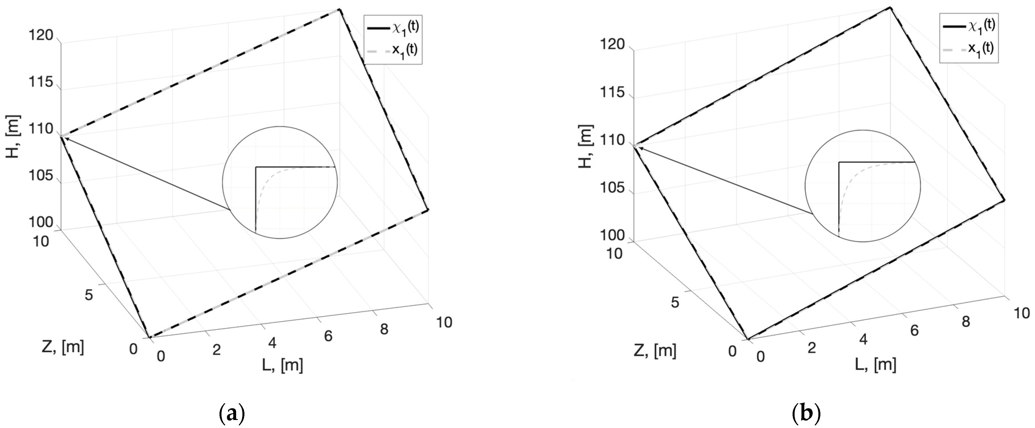
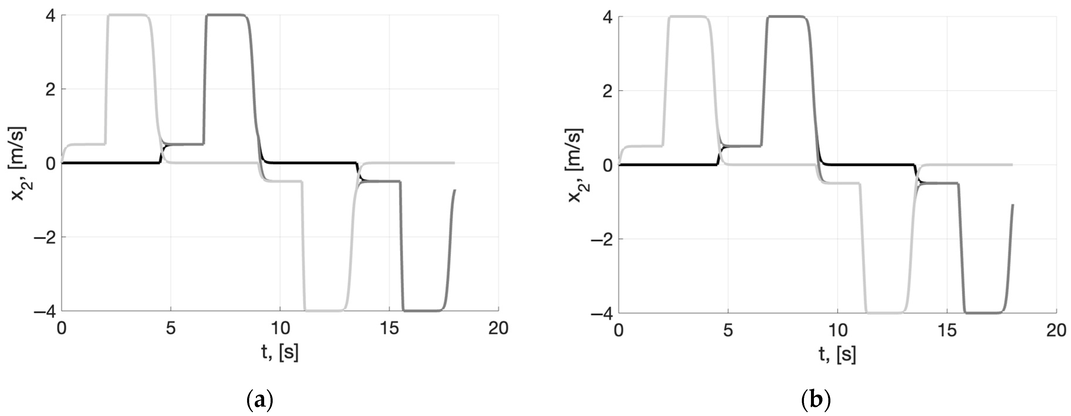
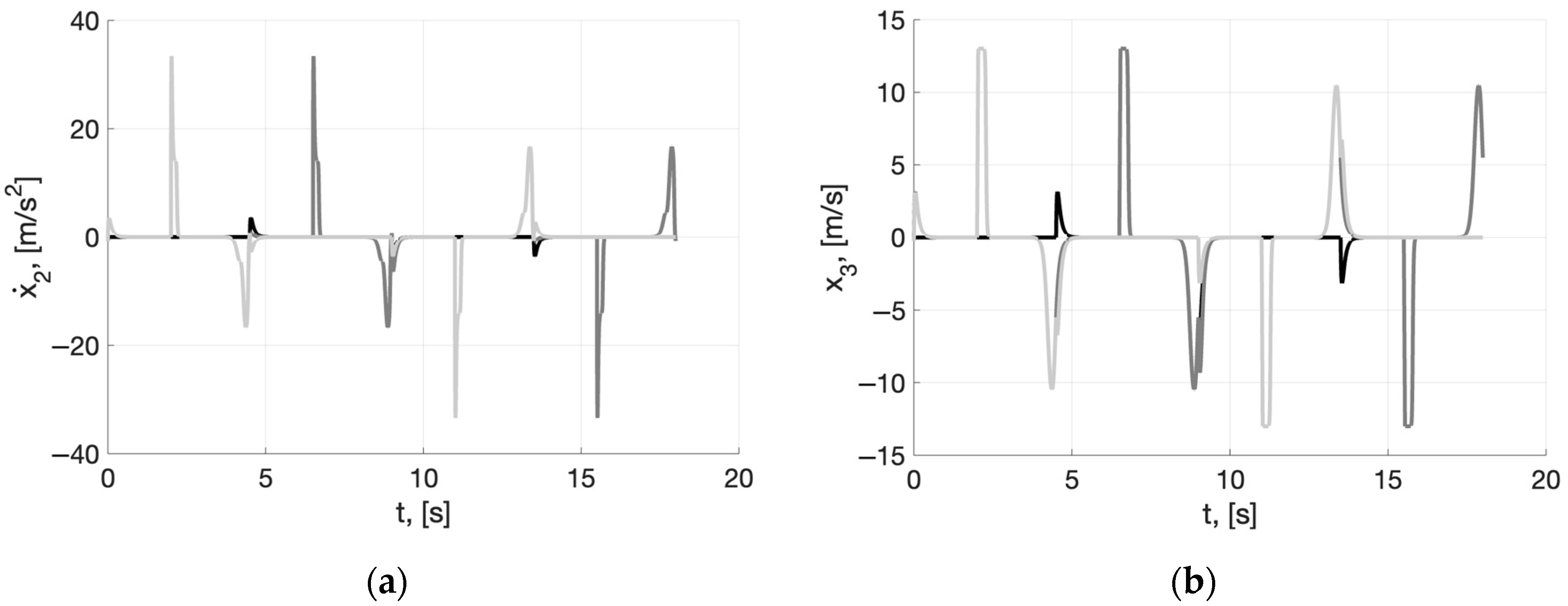
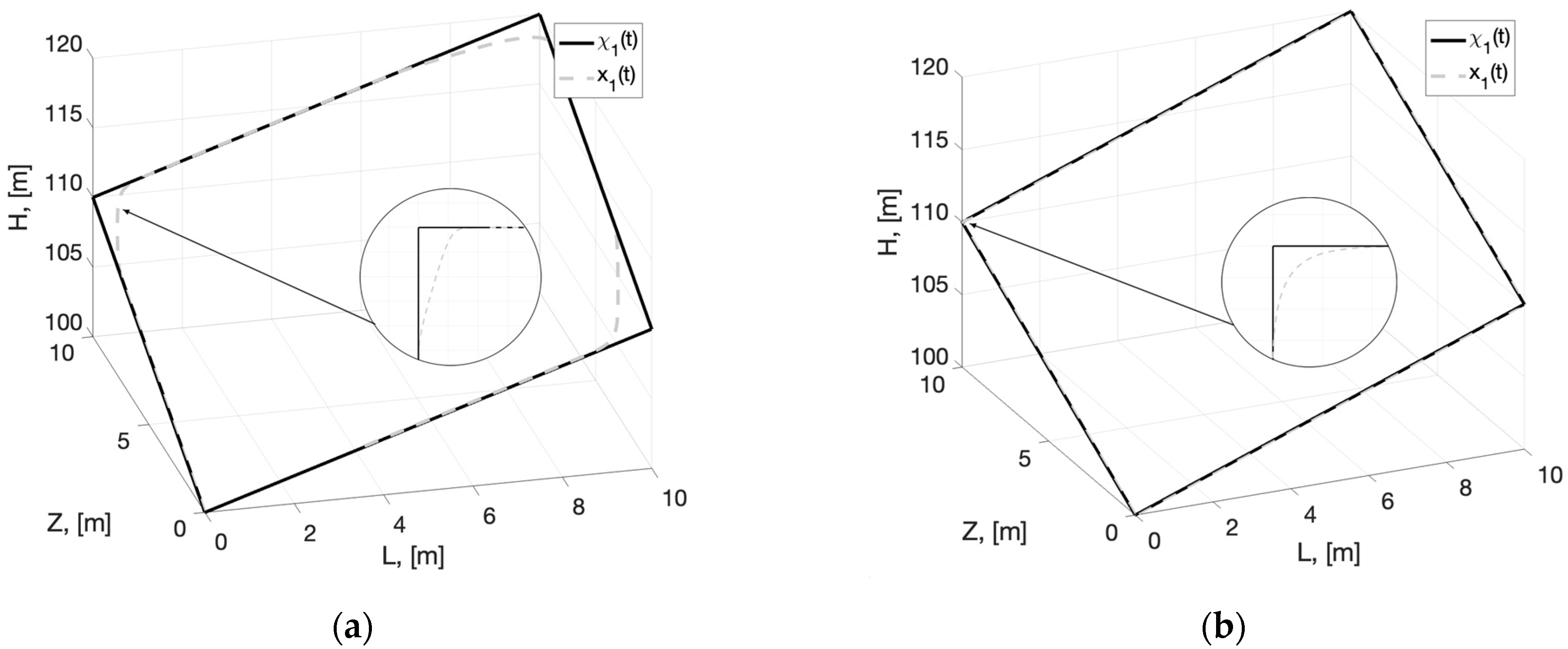
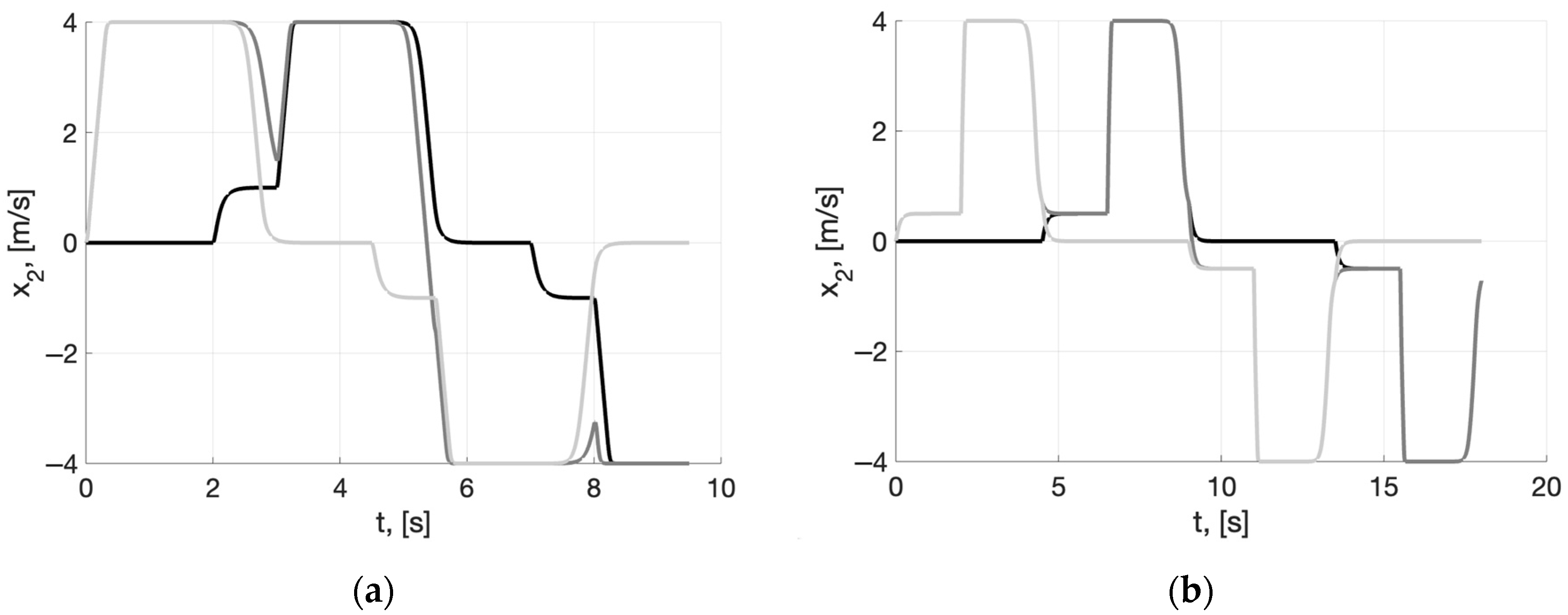
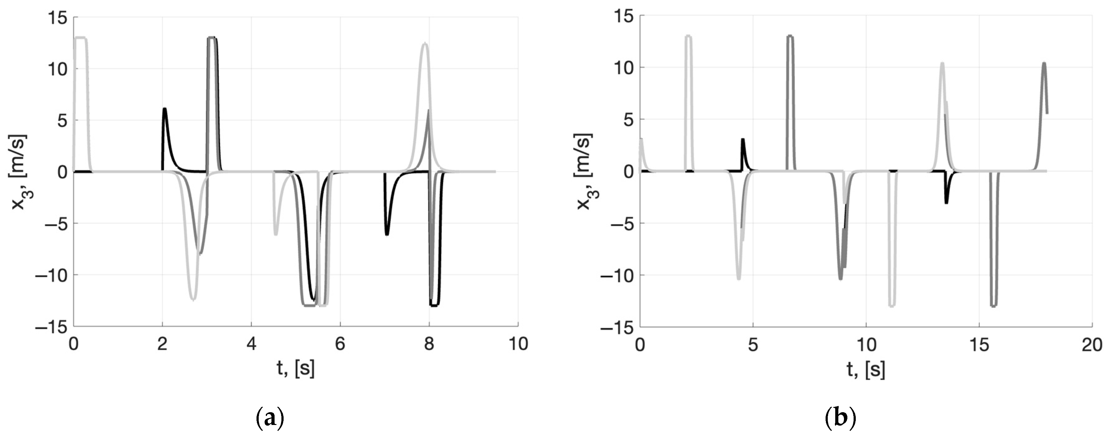
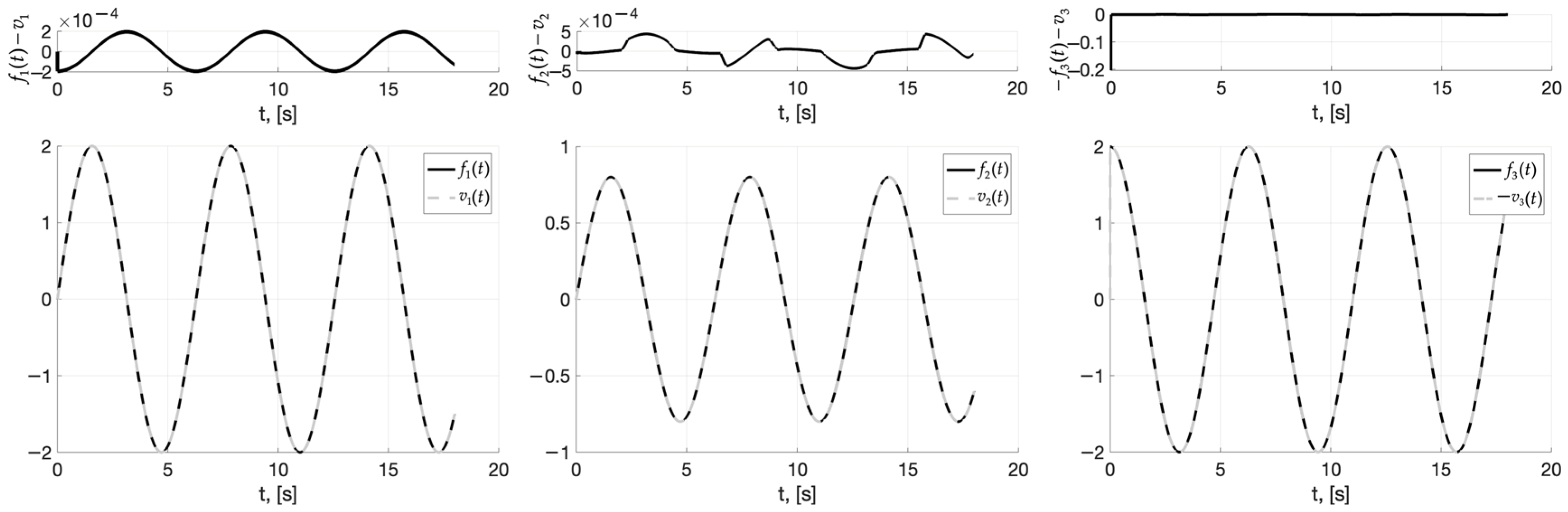
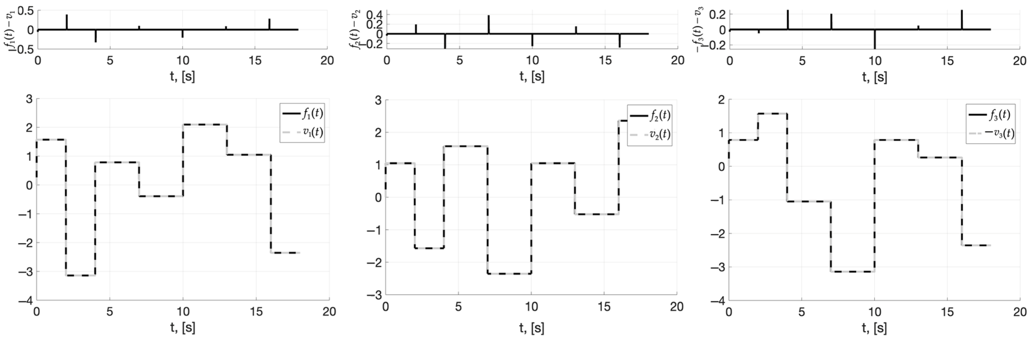
4. Numerical Simulation Results

The developed algorithms were numerically simulated using MATLAB-Simulink software integrating the Euler method with a constant step of 0.001 s. We have considered a micro-UAV as a control plant and presented its main features in

Table 1. Parameters of micro-UAV.

Parameter	Value
Maximum weight, kg	5
Maximum altitude, m	5000
Maximum flight velocity, m/s	26
Flight duration, min	60

. Such vehicles are usually used to monitor a monitored area and obtain information on the current situation.

We have taken a spatial rectangle in a trajectory coordinate system as the primitive path of the UAV in flight mode. On the sides of this rectangle, we selected 13 points $(L_i, H_i, Z_i),$ $(L_1, H_1, Z_1)=(L_{13}, H_{13}, Z_{13})$ and set two correct sequences of 4D-points $(L_i, H_i, Z_i, t_i)$ (14)–(15), which differ only by the last coordinate $t_i$ (see

Table 2. Coordinates of the reference 4D points.

i	Li, m	Hi, m	Zi, m	ti, s, (Case 1)	ti, s (Case 2)
1	0	100	0	0	0
2	0	101	1	2	1/9
3	0	109	9	2.5	1
4	0	110	10	4.5	2
5	1	111	10	6.5	3
6	9	119	10	7	3.5
7	10	120	10	9	4.5
8	10	119	9	11	5.5
9	10	111	1	11.5	6
10	10	110	0	13.5	7
11	9	109	0	15.5	8
12	1	101	0	16	8.5
13	0	100	0	18	9.5

).

As can be seen, in case 1, the flight time is longer and the average velocity is lower than in case 2. Based on the data in Table 2, non-smooth primitive trajectories are automatically calculated. For illustration, we show the corresponding reference actions for the output variables (16) for case 1

$$\begin{array}{l}{\chi }_{11}=0, {\chi }_{12}=t/2+100, {\chi }_{13}=t/2, t\in [0; 2);\\ {\chi }_{11}=0, {\chi }_{12}=16t+69, {\chi }_{13}=16t-31, t\in [2; 2.5);\\ {\chi }_{11}=0, {\chi }_{12}=t/2+107.75, {\chi }_{13}=t/2+7.75, t\in [2.5; 4.5);\\ {\chi }_{11}=t/2-2.25, {\chi }_{12}=t/2+107.75, {\chi }_{13}=10, t\in [4.5; 6.5);\\ {\chi }_{11}=16t-103, {\chi }_{12}=16t+7, {\chi }_{13}=10, t\in [6.5; 7);\\ {\chi }_{11}=t/2+5.5, {\chi }_{12}=t/2+115.5, {\chi }_{13}=10, t\in [7; 9);\\ {\chi }_{11}=10, {\chi }_{12}=-t/2+124.5, {\chi }_{13}=-t/2+14.5, t\in [9; 11);\\ {\chi }_{11}=10, {\chi }_{12}=-16t+295, {\chi }_{13}=-16t+185, t\in [11; 11.5);\\ {\chi }_{11}=10, {\chi }_{12}=-t/2+116.75, {\chi }_{13}=-t/2+6.75, t\in [11.5; 13.5);\\ {\chi }_{11}=-t/2+16.75, {\chi }_{12}=-t/2+116.75, {\chi }_{13}=0, t\in [13.5; 15.5);\\ {\chi }_{11}=-16t+257, {\chi }_{12}=-16t+357, {\chi }_{13}=0, t\in [15.5; 16);\\ {\chi }_{11}=-t/2+9, {\chi }_{12}=-t/2+109, {\chi }_{13}=0, t\in [16; 18);\\ {\chi }_{11}=t-18, {\chi }_{12}=100, {\chi }_{13}=t-18, t\ge 18, {\chi }_{ij} [m], t [s].\end{array}$$

(38)

and for case 2

$$\begin{array}{l}{\chi }_{11}=0, {\chi }_{12}=9t+100, {\chi }_{13}=9t, t\in [0; 1/9);\\ {\chi }_{11}=0, {\chi }_{12}=9t+100, {\chi }_{13}=9t, t\in [1/9; 1);\\ {\chi }_{11}=0, {\chi }_{12}=t+108, {\chi }_{13}=t+8, t\in [1; 2);\\ {\chi }_{11}=t-2, {\chi }_{12}=t+108, {\chi }_{13}=10, t\in [2; 3);\\ {\chi }_{11}=16t-47, {\chi }_{12}=16t+63, {\chi }_{13}=10, t\in [3; 3.5);\\ {\chi }_{11}=t+5.5, {\chi }_{12}=t+115.5, {\chi }_{13}=10, t\in [3.5; 4.5);\\ {\chi }_{11}=10, {\chi }_{12}=-t+124.5, {\chi }_{13}=-t+14.5, t\in [4.5; 5.5);\\ {\chi }_{11}=10, {\chi }_{12}=-16t+207, {\chi }_{13}=-16t+97, t\in [5.5; 6);\\ {\chi }_{11}=10, {\chi }_{12}=-t+117, {\chi }_{13}=-t+7, t\in [6; 7);\\ {\chi }_{11}=-t+17, {\chi }_{12}=-t+117, {\chi }_{13}=0, t\in [7; 8);\\ {\chi }_{11}=-16t+137, {\chi }_{12}=-16t+237, {\chi }_{13}=0, t\in [8; 8.5);\\ {\chi }_{11}=-t+9.5, {\chi }_{12}=-t+109.5, {\chi }_{13}=0, t\in [8.5; 9.5);\\ {\chi }_{11}=t-9.5, {\chi }_{12}=100, {\chi }_{13}=t-9.5, t\ge 9.5, {\chi }_{ij} [m], t [s].\end{array}$$

(39)

To smooth the primitive trajectories (38) and (39) we used a 9th-order tracking differentiator (28) with parameters

$$m_1=4, k_1=4 , m_2=13, k_2=8, m_3=350, k_3=10,$$

(40)

adopted from Equations (26) and (27) considering the constraints from Table 1.

To compare performance, we also used a 6th-order tracking differentiator [16,17] of the form

$$\begin{array}{l}{\dot{x}}_1=x_2, \\ {\dot{x}}_2=-m_2\sigma (k_2{e}_2)-0.5m_1{k}_1{\Lambda }_1{x}_2=-m_2\sigma (k_2(x_2+m_1\sigma (k_1(x_1-{\chi }_1))))-\\ -0.5m_1{k}_1\left(\begin{array}{ccc}1-{\sigma }^2(k_1(x_{11}-{\chi }_{11}))& 0& 0\\ 0& 1-{\sigma }^2(k_1((x_{12}-{\chi }_{12})))& 0\\ 0& 0& 1-{\sigma }^2(k_1((x_{13}-{\chi }_{13})))\end{array}\right)x_2\end{array}$$

(41)

with parameters $m_1=4, k_1=4 , m_2=14, k_2=10$ to smooth trajectories (38). The initial conditions $x_1(0), x_2(0)$ in both tracking differentiators (28), (41) are the same $x_1(0)={\chi }_1(0)={(0, 100, 0)}^{\mathrm{T}},$ $x_2(0)={(0.01, 0.01, 0.01)}^{\mathrm{T}};$ $x_3(0)={(0.01, 0.01, 0.01)}^{\mathrm{T}}$ for the system (28).

In the first series of experiments, we demonstrate the performance of tracking differentiators (28) and (41). For this, the reference action is primitive trajectory (38) and of the tracking differentiator (28), (40) when smoothing primitive trajectories (38) and (39).

Figure 1 shows the spatial plots of the primitive trajectory $({\chi }_{11}(t), {\chi }_{12}(t), {\chi }_{13}(t))$ (38) and the smooth trajectories $(x_{11}(t), x_{12}(t), x_{13}(t))$ obtained with order 6 tracking differentiator (41) (Figure 1a) and order 9 (28) (Figure 1b). Figure 2 and Figure 3 show the corresponding graphs of velocities $x_{21}(t), x_{22}(t), x_{23}(t)$ and accelerations ${\dot{x}}_{21}(t), {\dot{x}}_{22}(t), {\dot{x}}_{23}(t)$ (Figure 3a), $x_{31}(t), x_{32}(t), x_{33}(t)$ (Figure 3b) for both tracking differentiators.

It can be seen from Figure 1 and Figure 2 that both tracking differentiators effectively smooth the primitive trajectory (38) in the corners of the rectangle and that the velocity values $x_{2j}(t)$ are within acceptable limits. The plots of Figure 3 show that the quality of acceleration smoothing is the same for both cases. However, for the 9th-order tracking differentiator (28), the outliers at special points are about three times smaller than those for the 6th-order tracking differentiator (41), where acceleration values are taken not from the outputs but from the inputs of the integrators in the last block. At the same time, the counting time of the sixth order tracking differentiator (41) is 0.7 s. In the tracking differentiator (28), despite the higher order, the counting time was reduced to 0.6 s. It was achieved by using a purely sigmoid correcting action and a more simplified form of the last equation.

Figure 4, Figure 5 and Figure 6 show position, velocity, and acceleration plots similar to Figure 1, Figure 2 and Figure 3. We obtained them using a tracking differentiator (28) when smoothing the primitive trajectory (39) (left) and the primitive trajectory (38) (right). Note that the parameters of the corrective actions were the same in both cases (40), the tracking differentiator does not need to be reconfigured when the primitive trajectory is changed.

From the plots of Figure 4, Figure 5 and Figure 6, it can be concluded that the 9th-order tracking differentiator (28) gives good performance and provides constrained velocity and acceleration for tracking different trajectories. By reducing the velocity near special points in the planning phase, we can control the smoothing quality of the primitive trajectories and their derivatives.

In the following series of experiments, we demonstrate the performance of a closed-loop system (1) with dynamic feedback (37) with gains $c_1=4,$ $c_2=6$ and a disturbance observer (29). We use the variables of the tracking differentiator (28), (40), which track the primitive trajectory (38), as the attainable reference actions and their derivatives.

In the simulations, we considered two types of bounded external disturbances: smooth

$$f_1(t)=2\sin (t), f_2(t)=0.8\sin (t), f_3(t)=2\cos (t)$$

(42)

and non-smooth time functions

$$\begin{array}{l}{f}_1(t)=\pi /2, f_2(t)=\pi /3, f_3(t)=\pi /4, t\in [0; 2);\\ f_1(t)=-\pi , f_2(t)=-\pi /2, f_3(t)=\pi /2, t\in [0;4);\\ f_1(t)=\pi /4, f_2(t)=\pi /2, f_3(t)=-\pi /3, t\in [0; 7);\\ f_1(t)=-\pi /8, f_2(t)=-3\pi /4, f_3(t)=-\pi , t\in [0; 10);\\ f_1(T0)=2\pi /3, f_2(t)=\pi /3, f_3(t)=\pi /4, t\in [0; 13);\\ f_1(t)=\pi /3, f_2(t)=-\pi /6, f_3(t)=\pi /12, t\in [0; 16);\\ f_1(t)=-3\pi /4, f_2(t)=3\pi /4, f_3(t)=-3\pi /4, t\ge 16, t [s].\end{array}$$

(43)

Based on Equations (34) and (36), we have adopted the following values of amplitudes and high gains of sigmoid corrective actions (31) of the observer (29):

$$p_j=15, l_j=150 , j=\overline{1.3}.$$

(44)

Figure 7 and Figure 8 below show plots of disturbances $f_1(t),f_2(t),f_3(t)$ (42), (43), respectively, and their estimates $v_1(t), v_2(t), -v_3(t)$ obtained in the closed-loop system (1), (37) using observer (29), (44), and above show plots of estimation errors $f_1(t)-v_1(t),$ $f_2(t)-v_2(t),$ $-f_3(t)-v_3(t).$

As can be seen in Figure 7 and Figure 8, the disturbance observer (29) provided excellent performance in estimating both smooth (42) and non-smooth (43) disturbances. The observer operated without resetting, in both cases, we used the same amplitudes and high gains (44). In the case of smooth disturbances (42), the estimation errors are in the ranges

$$\left|f_1(t)-v_1(t)\right|\le 2\times {10}^{-4},\left|f_2(t)-v_2(t)\right|\le 5\times {10}^{-4},\left|-f_3(t)-v_3(t)\right|\le 2\times {10}^{-1}, t\ge 0,$$

and the steady-state errors are ${10}^{-3}-{10}^{-4}.$ In the case of non-smooth disturbances (43), the estimation errors are in the ranges

$$\left|f_1(t)-v_1(t)\right|\le 3.9\times {10}^{-1},\left|f_2(t)-v_2(t)\right|\le 3.9\times {10}^{-1},\left|-f_3(t)-v_3(t)\right|\le 2.6\times {10}^{-1}, t\ge 0,$$

and the steady-state errors are ${10}^{-13}-{10}^{-15}.$

In the following series of experiments, we demonstrate the performance of a closed-loop system (1) with dynamic feedback (37) with gains $c_1=4,$ $c_2=6$ and disturbance observer (29). We use the variables of tracking differentiator (28), (40) that track the primitive trajectory (38) as the reference actions and their derivatives.

For the closed-loop system (1), (28), (29), (37), (38) for the “worst case” of non-smooth disturbances (43) we obtain plots of tracking errors ${\xi }_1(t)=y_1(t)-x_1(t)={({\xi }_{11}(t), {\xi }_{12}(t), {\xi }_{13}(t))}^{\mathrm{T}}$ (Figure 9a) and plots of controls $u(t)={(u_1(t), u_2(t), u_3(t))}^{\mathrm{T}}$ (37) (Figure 9b).

From these plots, it can be seen that we have achieved the UAV control goal. In steady-state mode at $t\ge 2 s$ the tracking error ${\xi }_{1j}(t)$ is approximately ${10}^{-16}$– ${10}^{-7}$ m, and the maximum value of the tracking error does not exceed ${10}^{-3}$ m. The control actions do not exceed the admissible overloads and are in the ranges

$$\left|u(t)\right|\le 2.91,\left|u(t)\right|\le 1.31,\left|u_3(t)\right|\le 0.48, t\ge 0.$$

Thus, the simulation results confirmed the effectiveness of the designed algorithms.

5. Discussion

One of the sub-tasks of trajectory control is to plan the path or trajectory of an autonomous mobile robot in a workspace, in particular by setting waypoints and the desired ground velocity in different sections. In practice, however, tracking such primitive trajectories is often not possible due to the velocity and maneuverability constraints of the vehicles. Therefore, the next step is to smooth the primitive trajectory so that it is realizable by a specific mechanical plant. Known methods for smoothing primitive trajectories are based on the approximation of special sections by smooth analytical functions. There are three disadvantages to these approaches. First, the problem of providing constraints on the first and high derivatives of the reference action in these approaches requires additional testing and algorithmization. Second, the general complex of solved problems requires a large amount of computation and data memory, which constrains their implementation in the online mode. Third, it is not suitable in cases where the target conditions are not known in advance and are generated at the current point in time, for example, in pursuit/evasion problems.

We proposed a dynamic (automatic) smoothing method. The developed algorithms (tracking differentiator) generate achievable trajectories and their derivatives of any required order as signals. We do not aim at obtaining an analytical description, as this is not usually required for feedback design. At the same time, we ensure the implementability of the generated trajectory by matching the structure of the generator with the canonical model of the control plant and its corrective actions with the real controls. The design of corrective actions in the form of S-shaped smooth and bounded sigmoid functions enables us to consider the amplitude and growth rate constraints of real controls at the design stage. The application of the block method of design with the formation of sigmoid local feedback enables us to consider the same constraints on the phase variables too. Note that the developed algorithms are not intended for special cases where we should obtain a smoothed signal in analytical form or solve a boundary-value problem. In typical tracking problems where the analytical form of the reference signals is not required, our algorithms show better performance than the analytical smoothing methods mentioned above. They can be implemented in any software environment and do not require large computational resources. This method is also applicable to smooth signals obtained in real time from an autonomous source. However, unlike the design phase, we cannot adjust the initial data in online mode. If these data do not satisfy the initial requirements specified in Section 3.1, the results will be inadequate. If the initial data are acceptable, our algorithms are preferable to analytical approaches. They generate output signals quickly and produce less lag as the smoothed signals enter the controller.

In this paper, the generator of admissible trajectories is autonomous in relation to the control plant. It also does not explicitly consider the influence of external disturbances. We find it promising to use the current external disturbance information. Such information is obtained from the disturbance observer in the synthesis of a tracking differentiator to correct the trajectory generated in real time. Further development of this approach is also related to its application for generating admissible trajectories for other autonomous mobile robots (quadcopters, submersibles, etc.) considering their design features and operating environment. Moreover, in order to implement this in practice, it is necessary to consider a discrete implementation of the developed algorithms, which we have presented here in continuous time.

6. Conclusions

In this paper, we proposed a simple and efficient method for generating an achievable trajectory from given waypoints and a desired velocity for aircraft-type vehicles. The main idea of the proposed approach is to smooth the initial trajectory using a dynamic model (a tracking differentiator), considering the design constraints on the velocity and acceleration of the control object. We can also use only the current values of the reference signal.

We also proposed a method for real-time estimation of a wide class of external disturbances by sigmoid corrective actions of a disturbance observer of the lowest possible dimensionality. This approach, on the one hand, allows the recovery of unknown external actions with any given accuracy. On the other hand, it avoids strong surges in the estimated signals. We use this information to compensate for the influence of external disturbances on the plant using a combined control law. The simultaneous use of a tracking differentiator and a disturbance observer to design the dynamic feedback enabled us to implement a combined control law with a simple linear stabilizing component and provide asymptotic stabilization of tracking errors in a closed-loop system.

References

1. McGee, T.G.; Hedrick, J.K. Optimal Path Planning with a Kinematic Airplane Model. J. Guid. Control Dyn. 2007, 30, 629–633. [Google Scholar] [CrossRef]
2. Sujit, P.B.; Saripalli, S.; Sousa, J.B. Unmanned Aerial Vehicle Path Following: A Survey and Analysis of Algorithms for Fixed-Wing Unmanned Aerial Vehicles. IEEE Control Syst. 2014, 34, 42–59. [Google Scholar] [CrossRef]
3. Zhang, H.; Lin, W.; Chen, A. Path Planning for the Mobile Robot: A Review. Symmetry 2018, 10, 450. [Google Scholar] [CrossRef]
4. Campbell, S.; O’Mahony, N.; Carvalho, A.; Krpalkova, L.; Riordan, D.; Walsh, J. Path Planning Techniques for Mobile Robots A Review. In Proceedings of the 6th International Conference on Mechatronics and Robotics Engineering (ICMRE), Barcelona, Spain, 12–15 February 2020. [Google Scholar]
5. Zhou, C.; Huang, B.; Fränti, P. A review of motion planning algorithms for intelligent robots. J. Intell. Manuf. 2022, 33, 387–424. [Google Scholar] [CrossRef]
6. Imran, M.; Kunwar, F. A hybrid path planning technique developed by integrating global and local path planner. In Proceedings of the International Conference on Intelligent Systems Engineering (ICISE), Islamabad, Pakistan, 15–18 January 2016. [Google Scholar]
7. Yakovlev, K.; Andreychuk, A.; Belinskaya, J.; Makarov, D. Combining Safe Interval Path Planning and Constrained Path Following Control: Preliminary Results. Lect. Notes Comput. Sci. 2019, 11659, 310–319. [Google Scholar] [CrossRef]
8. Shin, Y.; Kim, E. Hybrid Path Planning Using Positioning Risk and Artificial Potential Fields. Aerosp. Sci. Technol. 2021, 112, 106640. [Google Scholar] [CrossRef]
9. Yuan, Q.; Yi, J.; Sun, R.; Bai, H. Path Planning of a Mechanical Arm Based on an Improved Artificial Potential Field and a Rapid Expansion Random Tree Hybrid Algorithm. Algorithms 2021, 14, 321. [Google Scholar] [CrossRef]
10. Pan, J.; Zhang, L.; Manocha, D. Collision-Free and Smooth Trajectory Computation in Cluttered Environments. Int. J. Robot. Res. 2012, 31, 1155–1175. [Google Scholar] [CrossRef]
11. Bautista, G.D.; Perez, J.; Milanés, V.; Nashashibi, F. A Review of Motion Planning Techniques for Automated Vehicles. IEEE Trans. Intell. Transp. Syst. 2015, 17, 1135–1145. [Google Scholar] [CrossRef]
12. Mercy, T.; Van Parys, R.; Pipeleers, G. Spline-Based Motion Planning for Autonomous Guided Vehicles in a Dynamic Environment. IEEE Trans. Control Syst. Technol. 2017, 26, 2182–2189. [Google Scholar] [CrossRef]
13. Lambert, E.D.; Romano, R.; Watling, D. Optimal Path Planning with Clothoid Curves for Passenger Comfort. In Proceedings of the 5th International Conference on Vehicle Technology and Intelligent Transport Systems, Heraklion, Greece, 3–5 May 2019. [Google Scholar]
14. Rosu, H.C.; Mancas, S.C.; Hsieh, C.-C. Generalized Cornu-Type Spirals and their Darboux Parametric Deformations. Phys. Lett. A 2019, 383, 2692–2697. [Google Scholar] [CrossRef]
15. Kano, H.; Fujioka, H. B-Spline Trajectory Planning with Curvature Constraint. In Proceedings of the Proceeding on the Annual American Control Conference (ACC), Milwaukee, WI, USA, 27–29 June 2018. [Google Scholar]
16. Antipov, A.S.; Kokunko, Y.G.; Krasnova, S.A. Dynamic Model Design for Processing Motion Reference Signals for Mobile Robots. J. Intell. Robot. Syst. 2022, 105, 77. [Google Scholar] [CrossRef]
17. Antipov, A.S.; Kokunko, J.G.; Krasnova, S.A.; Utkin, V.A. Dynamic Smoothing, Filtering and Differentiation of Signals Defining the Path of the UAV. Sensors 2022, 22, 9472. [Google Scholar] [CrossRef]
18. Guo, B.-Z.; Zhao, Z.-L. On Convergence of Tracking Differentiator and Application to Frequency Estimation of Sinusoidal Signals. In Proceedings of the 8th Asian Control Conference (ASCC), Kaohsiung, Taiwan, 15–18 May 2011. [Google Scholar]
19. Park, S.; Han, S. Robust Super-Twisting Sliding Mode Backstepping Control Blended with Tracking Differentiator and Nonlinear Disturbance Observer for an Unknown UAV System. Appl. Sci. 2022, 12, 2490. [Google Scholar] [CrossRef]
20. Kochetkov, S.A.; Krasnova, S.A.; Antipov, A.S. Cascade Synthesis of Electromechanical Tracking Systems with Respect to Restrictions on State Variables. IFAC-PapersOnLine 2017, 50, 1042–1047. [Google Scholar] [CrossRef]
21. Antipov, A.S.; Krasnova, S.A.; Utkin, V.A. Synthesis of Invariant Nonlinear Single-Channel Sigmoid Feedback Tracking Systems Ensuring Given Tracking Accuracy. Autom. Remote Control 2022, 83, 32–53. [Google Scholar] [CrossRef]
22. Miele, A.; Wang, T.; Melvin, W.W. Optimal Take-off Trajectories in the Presence of Windshear. J. Optim. Theory Appl. 1986, 49, 1–45. [Google Scholar] [CrossRef]
23. Botkin, N.; Turova, V.; Diepolder, J.; Holzapfel, F. Computation of Viability Kernels on Grid Computers for Aircraft Control in Windshear. Adv. Sci. Technol. Eng. Syst. J. 2018, 3, 502–510. [Google Scholar] [CrossRef]
24. Etienne, L.; Hetel, L.; Efimov, D. Observer Analysis and Synthesis for Perturbed Lipschitz Systems under Noisy Time-Varying Measurements. Automatica 2019, 106, 406–410. [Google Scholar] [CrossRef]
25. Zhang, W.; Wang, Z.; Raïssi, N.; Shen, Y. Ellipsoid-Based Interval Estimation for Lipschitz Nonlinear Systems. IEEE Trans. Autom. Control 2022, 67, 6802–6809. [Google Scholar] [CrossRef]
26. Leitmann, G.; Pandey, S. Adaptive control of aircraft in windshear. Int. J. Robust Nonlinear Control 1993, 3, 133–153. [Google Scholar] [CrossRef]
27. Hasibuan, J.R.P.D.; Yulia, E.; Barri, M.H.; Widyotriatmo, A. Control of Nonlinear System with State-Constraints using Barrier Lyapunov Function and Backstepping Method. Int. J. Control Autom. 2018, 11, 165–174. [Google Scholar] [CrossRef]
28. Delshad, S.S.; Johansson, A.; Darouach, M.; Gustafsson, T. Robust State Estimation and Unknown Inputs Reconstruction for a Class of Nonlinear Systems: Multiobjective Approach. Automatica 2016, 64, 1–7. [Google Scholar] [CrossRef]
29. Nikiforov, V.O. Adaptive nonlinear tracking with complete compensation of unknown disturbances. Eur. J. Control 1998, 4, 132–139. [Google Scholar] [CrossRef]
30. Andrievsky, B.R.; Furtat, I.B. Disturbance Observers: Methods and Applications. I. Methods. Autom. Remote Control 2020, 81, 1563–1610. [Google Scholar] [CrossRef]
31. Wang, H.; Zhang, Z.; Tang, X.; Zhao, Z.; Yan, Y. Continuous Output Feedback Sliding Mode Control for Underactuated Flexible-Joint Robot. J. Frankl. Inst. 2022, 359, 7847–7865. [Google Scholar] [CrossRef]
32. Kikuuwe, R.; Pasaribu, R.; Byun, G.A. First-Order Differentiator with First-Order Sliding Mode Filtering. IFAC-Pap. 2019, 52, 771–776. [Google Scholar] [CrossRef]
33. Xu, D.; Liu, Z.; Zhou, X.; Yang, L.; Huang, L. Trajectory Tracking of Underactuated Unmanned Surface Vessels: Non-Singular Terminal Sliding Control with Nonlinear Disturbance Observer. Appl. Sci. 2022, 12, 3004. [Google Scholar] [CrossRef]
34. Basin, M.; Yu, P.; Shtessel, Y. Finite and Fixed-time Differentiators Utilising HOSM Techniques. IET Control Theory Appl. 2017, 11, 1144–1152. [Google Scholar] [CrossRef]
35. Krasnova, S.A.; Utkin, A.V. Sigma Function in Observer Design for States and Perturbations. Autom. Remote Control 2016, 77, 1676–1688. [Google Scholar] [CrossRef]
36. Krasnov, D.V.; Utkin, A.V. Synthesis of a Multifunctional Tracking System in Conditions of Uncertainty. Autom. Remote Control 2019, 80, 1704–1716. [Google Scholar] [CrossRef]
37. Krasnova, S.A. Estimating the Derivatives of External Perturbations Based on Virtual Dynamic Models. Autom. Remote Control 2020, 81, 897–910. [Google Scholar] [CrossRef]
38. Kokunko, Y.; Krasnova, S. Synthesis of a Tracking System with Restrictions on UAV State Variables. Math. Eng. Sci. Aerosp. MESA 2019, 10, 695–705. [Google Scholar]
39. Kanatnikov, A.N.; Krishchenko, A.P. Terminal control of spatial motion of flying vehicles. J. Comput. Syst. Sci. Int. 2008, 47, 718–731. [Google Scholar] [CrossRef]
40. Eldeeb, E.; Sant’Ana, J.M.D.S.; Pérez, D.E.; Shehab, M.; Mahmood, N.H.; Alves, H. Multi-UAV Path Learning for Age and Power Optimization in IoT with UAV Battery Recharge. IEEE Trans. Veh. Technol. 2023, 72, 5356–5360. [Google Scholar] [CrossRef]
Figure 1. Spatial plots of the primitive trajectory χ 1 ( t ) (38) and smoothed trajectories x 1 ( t ) obtained via tracking differentiator (41) in (a), and tracking differentiator (28) in (b).
Electronics 12 02280 g001
Figure 2. Plots of velocities x 21 ( t ) ,   x 22 ( t ) ,     x 23 ( t ) . In (a), for the tracking differentiator (41). In (b), for the tracking differentiator (28).
Electronics 12 02280 g002
Figure 3. Plots of accelerations. In (a), plots of x ˙ 21 ( t ) ,   x ˙ 22 ( t ) ,     x ˙ 23 ( t ) of the tracking differentiator (41). In (b), plots of x 31 ( t ) ,   x 32 ( t ) ,     x 33 ( t ) of the tracking differentiator (28).
Electronics 12 02280 g003
Figure 4. In (a), spatial plots of the primitive trajectory χ 1 ( t ) (39) and smooth trajectory x 1 ( t ) , obtained via tracking differentiator (28), (40). In (b), spatial plots of the primitive trajectory χ 1 ( t ) (38) and smooth trajectory x 1 ( t ) , obtained via tracking differentiator (28), (40).
Electronics 12 02280 g004
Figure 5. Plots of velocities x 21 ( t ) ,   x 22 ( t ) ,     x 23 ( t ) of the tracking differentiator (28), (40), obtained when tracking the primitive trajectory (39) in (a), and when tracking the primitive trajectory (38) in (b).
Electronics 12 02280 g005
Figure 6. Plots of accelerations x 31 ( t ) ,   x 32 ( t ) ,     x 33 ( t ) of the tracking differentiator (28), (40), obtained when tracking the primitive trajectory (39) in (a), and when tracking the primitive trajectory (38) in (b).
Electronics 12 02280 g006
Figure 7. Plots of the smooth external disturbances f 1 ( t ) , f 2 ( t ) , f 3 ( t ) (42) and their estimates v 1 ( t ) ,   v 2 ( t ) ,   v 3 ( t ) (shown below) and estimation errors f 1 ( t ) v 1 ( t ) ,   f 2 ( t ) v 2 ( t ) ,     f 3 ( t ) v 3 ( t ) (shown above).
Electronics 12 02280 g007
Figure 8. Plots of the non-smooth external disturbances f 1 ( t ) , f 2 ( t ) , f 3 ( t ) (43) and their estimates v 1 ( t ) ,   v 2 ( t ) ,   v 3 ( t ) (shown below) and estimation errors f 1 ( t ) v 1 ( t ) ,   f 2 ( t ) v 2 ( t ) ,     f 3 ( t ) v 3 ( t ) (shown above).
Electronics 12 02280 g008
Figure 9. In (a), plots of the tracking errors ξ 11 ( t ) ,   ξ 12 ( t ) ,   ξ 13 ( t ) . In (b), plots of the controls u 1 ( t ) ,   u 2 ( t ) ,   u 3 ( t ) .
Electronics 12 02280 g009