Abstract
Identifying the as-drilled location of blastholes is crucial for achieving optimal blasting results. This research proposes a novel integrated methodology to control drilling accuracy in open-pit mines. This approach is developed by combining aerial drone images with machine learning techniques. The study investigates the viability of photogrammetry combined with machine learning techniques, particularly Support Vector Machine (SVM) and Convolutional Neural Networks (CNN), for automatically detecting blastholes in photogrammetry representations of blast patterns. To verify the hypothesis that machine learning can detect blastholes in images as effectively as humans, various datasets (drone images) were obtained from different mine sites in Nevada, USA. The images were processed to create photogrammetry mapping of the drill patterns. In this process, thousands of patches were extracted and augmented from the photogrammetry representations. Those patches were then used to train and test different CNN architectures optimized to locate blastholes. After reaching an acceptable level of accuracy during the training process, the model was tested using a piece of completely unknown data (testing dataset). The high recall, precision, and percentage of detected blastholes prove that the combination of SVM, CNN, and photogrammetry (PHG) is an effective methodology for detecting blastholes on photogrammetry maps.
1. Introduction
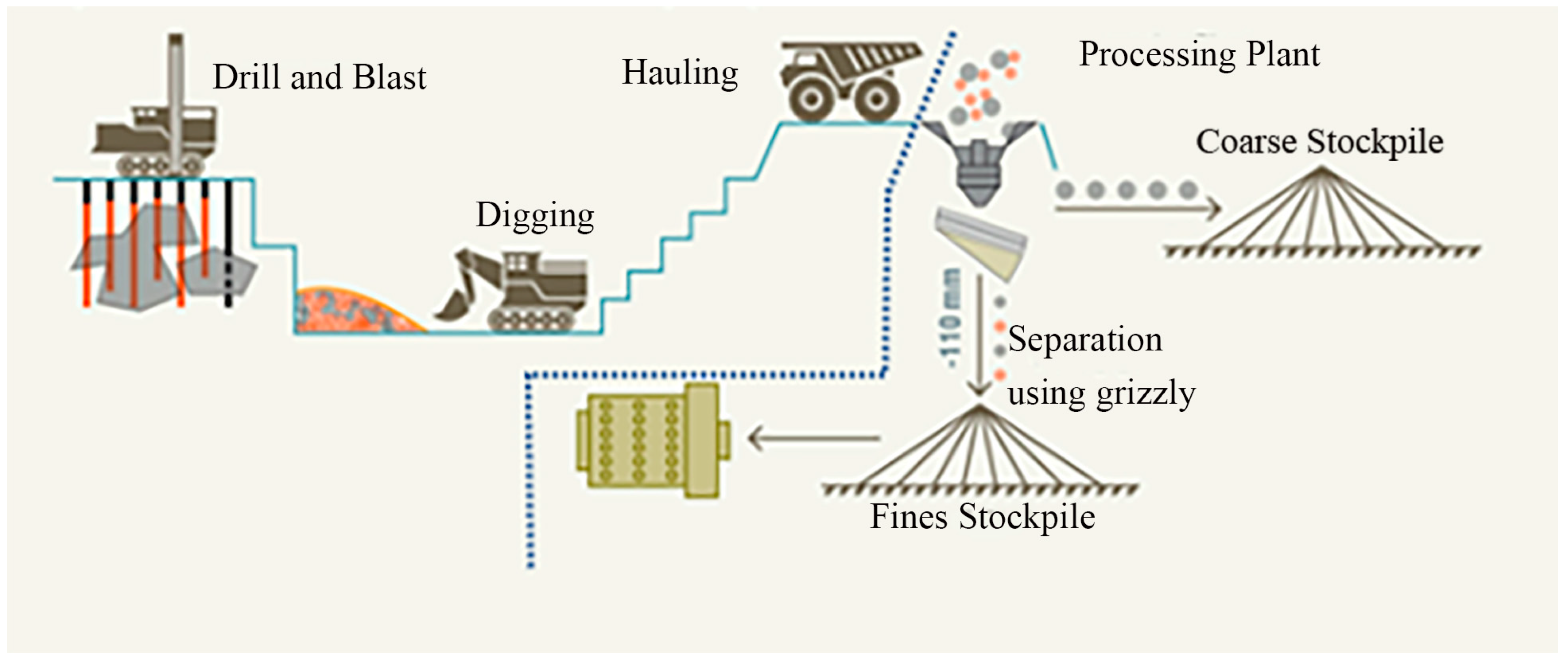
Figure 1 shows a simplified mining flowsheet where the first activity is drilling the in-situ rock, followed by blasting, then digging, hauling, and finally processing the ore. Drill and blast activities impact all these processes in a mine, influencing shovel productivity, equipment maintenance, highwall stability, ore recovery, and the related costs across all these processes. Therefore, it is necessary to utilize novel technologies, such as sensors, unmanned aerial vehicle (UAV), image processing, virtual reality, and teleoperation to address these issues [1,2,3,4].
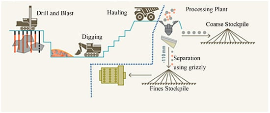
Figure 1.
An overview of key stages involved in ore processing [5].
Every blast in open-pit mines consists of hundreds of holes that sometimes deviate from their designed coordinates for diverse reasons, such as issues in the existing technologies of the drill rigs or low GPS signal. Moreover, blasthole collar inaccuracy leads to an imbalanced distribution of the explosive energy in the rock mass, resulting in unexpected blasting results. Even with high-precision GPS technologies onboard the most modern open-pit drilling machines, there is a considerable amount of (mostly unknown) collar deviations. This issue is mainly due to several factors: (i) some mine sites cannot or do not want to afford high precision RTK/GPS advanced features on their drill rigs, (ii) most of the small drill rigs (especially the ones intended to drill pre-split) are not equipped with high precision RTK/GPS, (iii) GPS accuracy decreases in locations close to high walls due to signal blocking, and (iv) drilling operators decide to make slight location changes to some blastholes due to operative reasons (e.g., pit edge, and overbreak from the previous blast). These operative changes are not always reflected in the final blasting decisions (e.g., explosive loading maps/spreadsheets). Although surveying is one of the most accurate methods for checking the blasthole location, it is not viable in current mining operations due to the time involved in the activity and the workforce needed. Therefore, drill and blast engineers usually have limited to no accurate data about the magnitude of the deviation in their drilled patterns. This paper proposes a new methodology to identify drilling collar errors using drones and machine learning techniques. This approach begins by capturing high-resolution images, which are processed first with photogrammetry techniques, and then using deep learning. Machine learning solves several imaging problems, including detection, segmentation, etc. Moreover, using machine learning to detect blastholes on aerial images can help control the drilling accuracy for better blasting outcomes, benefiting the downstream processes (e.g., digging, hauling, and ore processing).
Blasthole detection using drones and machine learning aims to be a complementary or supplementary way to know the blasthole location to improve the distribution of explosive energy in the blasting process. In open-pit mines, drill and blast engineers are interested in knowing the final location of the blastholes, but the information coming from this research may also be helpful for other departments like ore control and survey.
Mining engineers need to know the final location of the collar of the blastholes to adjust the blasting variables in the best possible way before executing the blast. Several blast variables can be improved using blasthole detection, such as powder factor, stemming depth, explosive type, and timing. The motivations behind developing an alternative system to manage the drilling accuracy through photogrammetry and machine learning are summarized as follows:
- Importance of drilling accuracy in blasting: Drilling accuracy is the main variable influencing blasting results.
- GPS signal loss: The inconvenience with the GPS mounted on the drilling machines is the loss of signal in some regions of the mine (blind spots), like close to the high walls. The quality of the signal received from the satellites relies on several elements, such as geometry/triangulation regarding the satellites, signal obstruction, atmospheric conditions, and features/technology of the receptor [6].
- Explosive energy distribution: To obtain good rock fragmentation and avoid issues (e.g., flyrocks, misfires, and oversize), it is essential to simulate the explosive energy distribution knowing the blasthole’s final location [7].
- Potential of the research: This research has great potential to be applied to other related object detection problems in the mining industry.
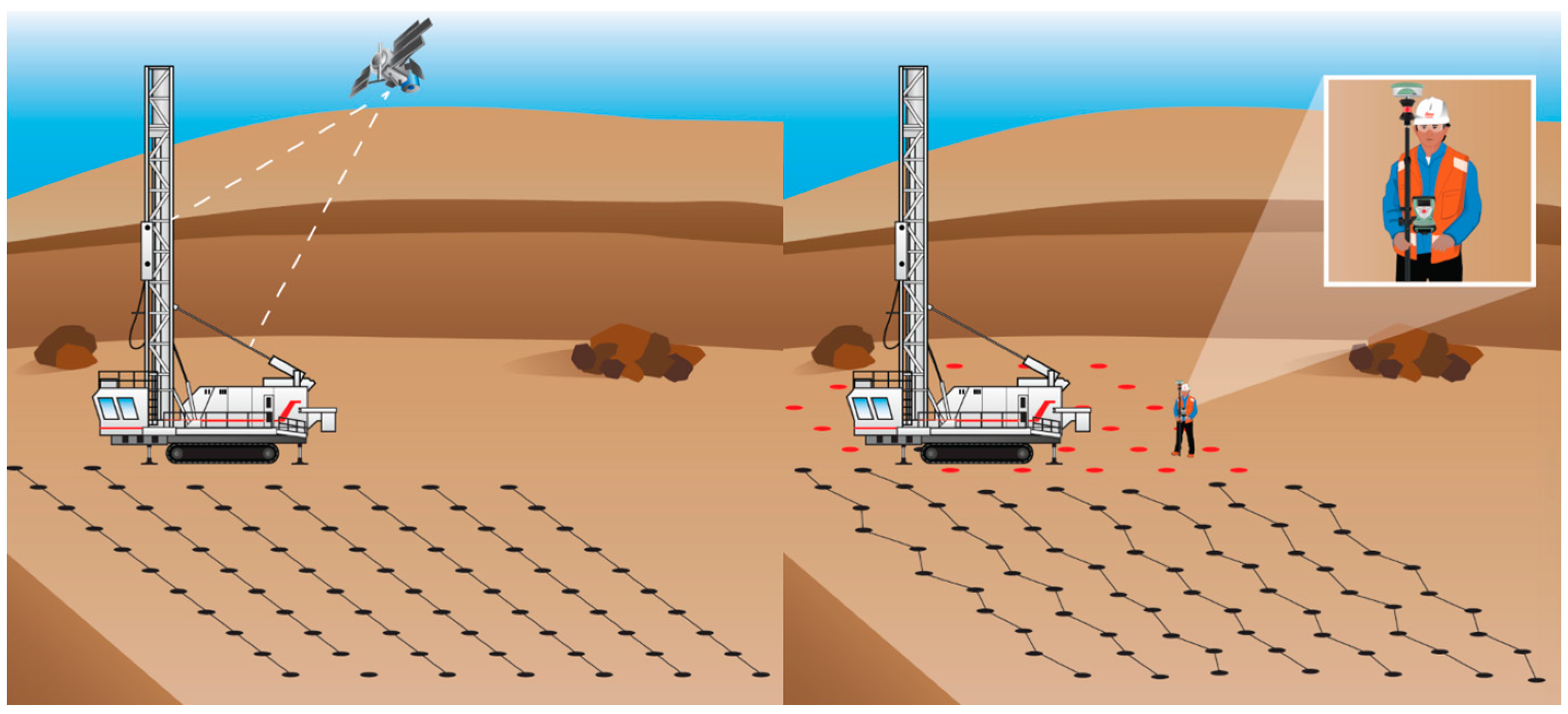
Figure 2, Figure 3 and Figure 4 show comparisons of the design of the pattern versus the on-field execution.

Figure 2.
Designing drill pattern using GPS (Left image) and implementing drill pattern being surveyed (Right image) [8].
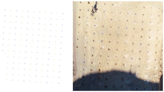
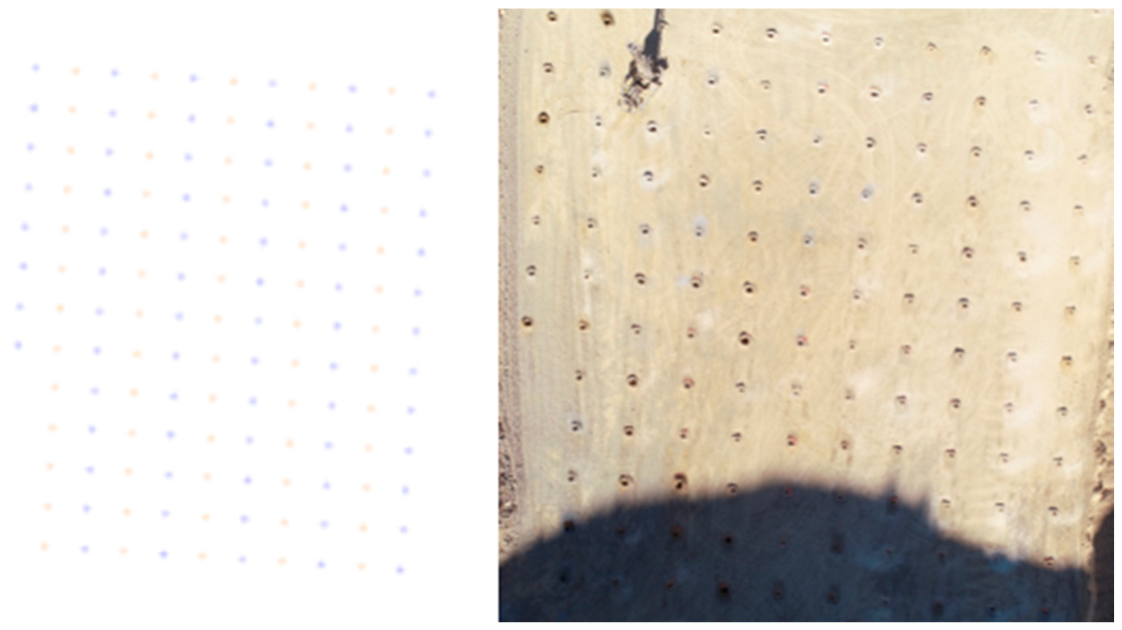
Figure 3.
Drilling pattern “as designed” (left) versus “as drilled” (right).
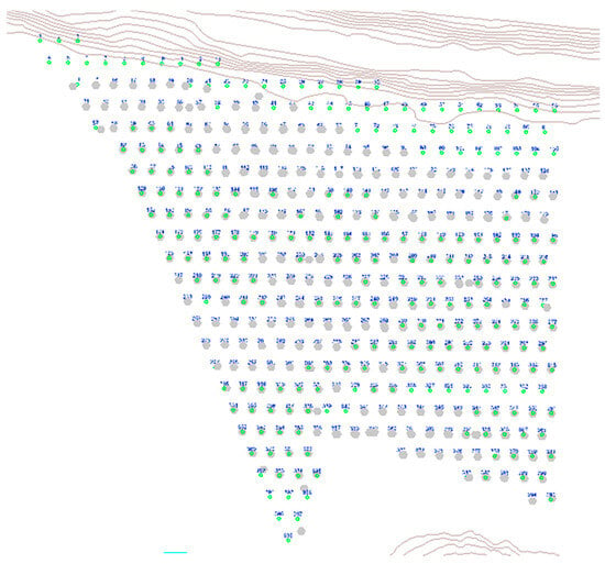
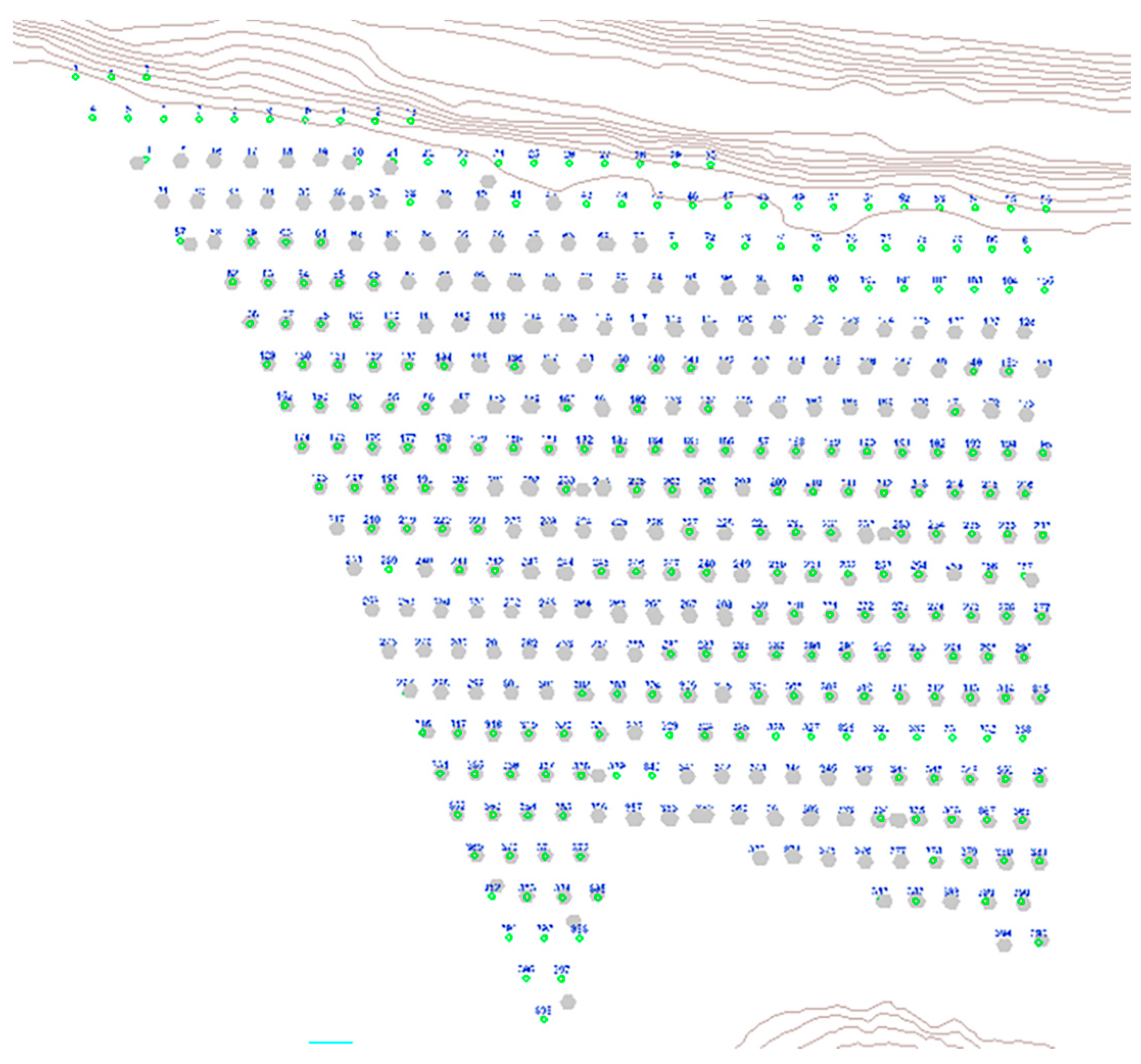
Figure 4.
“As designed” (green circles) versus “as drilled” (gray dots) reported by the high-precision GPS drilling system.
Figure 2 illustrates the two most common alternatives to obtain the final location of the blastholes, either GPS in the drill rigs or a survey. To the left, the machine drills the holes according to a drilling design perfectly aligned with the GPS, but the final implementation of the pattern is not always accurate, which can be verified through a survey. The left image in Figure 2 faces issues in some geographical locations or areas of the mine. In contrast, the right image in Figure 2 is highly time-consuming. Figure 3 depicts the drilling patterns “as designed” and “as drilled” in the field. Also, Figure 4 indicates a real case of a drill pattern. In this figure, “as designed” (green circles) and “as drilled” (gray dots) are performed by a high-precision GPS drilling system.
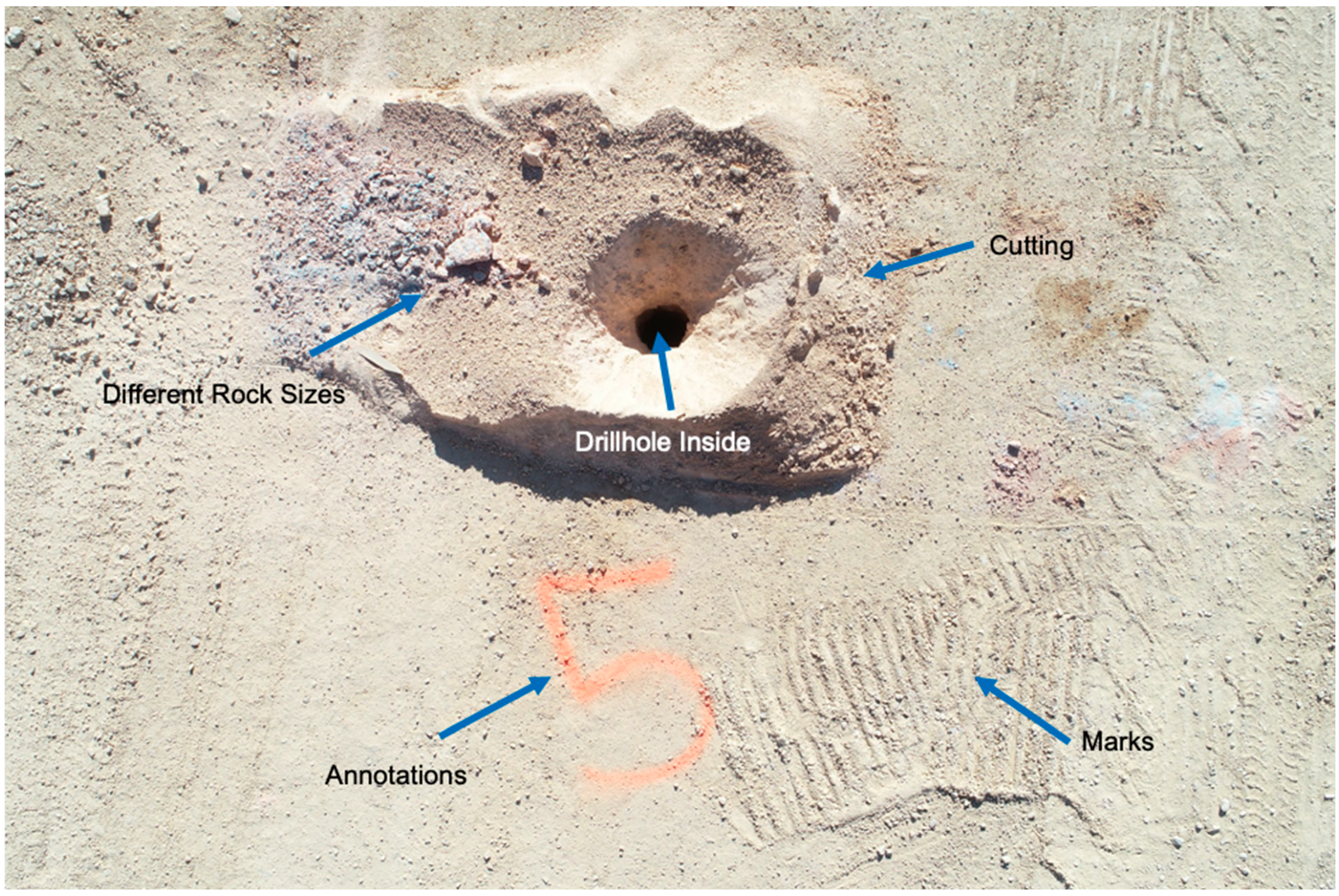
Blasthole detection over aerial images is challenging for machine learning algorithms because of different “distractions” in the drill pattern images, such as rocks, cutting (material coming from inside of the hole while being drilled), vehicle tracks, blasting accessories (primes and detonators), oil on the ground, and stakes (Figure 5).
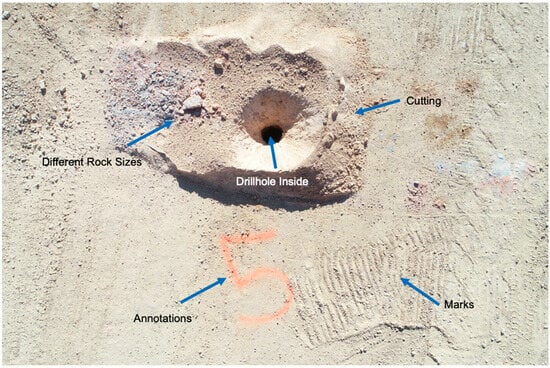
Figure 5.
A typical blasthole view from the air (10 ft above the ground level) with many features in the image like vehicle footprint, cutting, rocks, marks, shadows, etc.
In this paper, support vector machines and convolutional neural networks are proposed to solve the blasthole detection problem on drone aerial images converted or processed as Orthomosaic and DEM. The contributions of the present study are outlined as follows:
- New methodology to control drilling accuracy: Introducing a complementary or supplementary system to determine the final location of blastholes in cases where the GPS of the drills is inaccurate, has a poor signal, is uncalibrated, or the machine lacks GPS technology (e.g., pre-split drill rigs or older machines without the technology).
- New approach for object detection using Digital Elevation Models (DEM): Unlike most object detection techniques that use RGB or grayscale images, the proposed methodology, especially the multiple dataset stage, employs elevation data to detect the object of interest (blastholes).
- Providing a new tool to improve blasting results by developing more realistic process simulations.
- Establishing the first blasthole image database could lead to a more extensive blasthole image database from multiple mine sites.
The rest of the paper is organized as follows: Section 2 presents the related previous studies. Section 3 details the materials and methods used for this study, including the methodology for data collection, processing of raw data, experimentation with machine learning algorithms, and the framework employed. The results and discussion of the study are presented in Section 4. Section 5 provides the conclusions of the present study, along with its potential applications and future work.
2. Related Work
To the best of our knowledge, no specific references were found in the literature related to blasthole detection using photogrammetry and machine learning. However, a few studies have addressed blasthole detection on images. In [9], the authors utilized 205 RGB images from different mine sites, enhancing image quality through a “Blasthole Feature Extract Transformation” (BFET) module. They employed a YOLOv7 neural network architecture to develop models for blasthole detection. In [10], the authors developed a semi-supervised method using RGB-D images for blasthole segmentation, circumventing the need for manual annotation due to limited labeled data in mining. This approach employs pseudo-labeling with the histogram of gradients and self-training on unannotated images for segmentation.
Machine learning has recently been utilized in various aspects of drill and blast operations to develop more site-specific models. Researchers demonstrated that its estimation results were better than traditional methods [11,12,13,14,15,16,17,18,19,20,21,22,23,24,25,26]. In [27], the authors employed the Random Forest (RF) technique for estimating blast-induced ground vibration (BIGV). Amnieh et al. [28] utilized vibration measurement datasets from a copper mine to analyze the potential of Neural Networks in predicting BIGV during blasting operations. Also, Monjezi et al. [21] employed Neural Networks to predict fragmentation and flyrock during blasting operations. In [29], a methodology was developed to predict flyrocks using multivariate regression analysis (MVRA) and backpropagation neural network (BPNN). This methodology involved the motion analysis of 95 blast movies from four mines. In [30], the authors described several options to predict rockburst using machine learning. Among the techniques described in the study, they used the General Regression Neural Network (GRNN), Swarm Optimization, and Genetic Algorithm. Eades and Perry [31] established a deep belief model to differentiate Microseismic events from blasting signals. Shi et al. [32] applied Support vector machines (SVM) to predict fragmentation patterns after bench blasting operations. Another use of machine learning involves the estimation of NOX generated by blasting [33]. Furthermore, Jha and Tukkaraja [34] have focused on semantic segmentation to detect the geological discontinuities in open-pit mines using drone images and Convolutional Neural Network (CNN). A comprehensive review of the utilization of machine learning in predicting the broad domain of the blast impact was developed in another research study [35].
Cazzato et al. [36] examined recent advancements in 2D object detection for UAVs, emphasizing the utilization of RGB cameras due to their cost-effectiveness. They highlighted the importance of achieving autonomy and addressing operational challenges in UAV operations. Additionally, they proposed a new taxonomy based on height intervals and methodological approaches to categorize research in this field. Somua-Gyimah et al. [37] introduced a scalable machine vision model based on Convolutional Neural Networks for dragline excavation, achieving an average classification accuracy of 82.6% and 91% detection accuracy in collision avoidance. They also performed well in terrain recognition and oversized rock detection tasks, offering potential for broader application across automated excavators. Maitre et al. [38] presented a computational approach for automating mineral grain recognition from optical microscope images, offering a cost-effective alternative to manual characterization. Utilizing simple linear iterative clustering segmentation, the method efficiently isolates sand grains, demonstrating approximately 90% accuracy in mineral recognition.
According to the literature review, a few studies have focused on blasthole detection, particularly utilizing image processing techniques. However, these studies predominantly relied on image analysis using RGB or RGB-D images and did not incorporate photogrammetry techniques, which are essential for capturing detailed spatial information crucial for accurate blasthole detection. The study performed by [9] solely relied on the YOLOv7 neural network architecture, while the other study utilized a semi-supervised machine learning method based on pseudo-labeling using Histogram of Gradients. These approaches may not fully exploit the potential of combining different machine learning techniques for improved accuracy and reliability.
3. Materials and Methods
Deep learning (DL) is an advanced branch of machine learning that can find patterns in data that are not easy to recognize by humans. DL uses multiple layers to extract features at different levels or layers progressively. For example, lower layers may identify edges, while higher layers may identify some elements relevant to humans, such as digits, letters, or faces [39]. The solution proposed in this document uses deep learning to detect blastholes in photogrammetry representations (Orthomosaic and DEM). The data were collected at different mine sites located in Nevada, USA. These photogrammetry representations were used to train neural networks to detect blastholes in blasting patterns. Blasthole detections are challenging for automated algorithms due to the many features typically present in drilling images, such as cracks, cutting, rocks, and shadows (Figure 5).
3.1. Framework
Figure 6 illustrates the different stages involved in the proposed solution. The process starts by using drones to capture high-resolution images from the drilling areas. Then, those images are processed through photogrammetry techniques to generate Orthomosaic (union of individual images) and DEM (elevation maps). Next, a conventional drone (i.e., UAV) was used to take high-resolution pictures flying close to the holes (e.g., 40 feet = 12 m above the ground level (AGL)). A special ground control application was used for this step. Then, training and testing areas were defined for the single dataset stage. In the multiple dataset stage, one complete dataset was used for testing, and the remaining datasets were used for training. The training step starts with the annotation of the blastholes, involving drawing bounding boxes around the holes to teach algorithms the features of a blasthole. Through several examples, the algorithm can be learned from the data. In this case, the machine learning algorithm was trained to differentiate between blastholes and no-blastholes using patches extracted from the photogrammetry representations containing positive samples (blastholes) and negative samples. The patches were then augmented using different techniques, including rotations, translations, and brightness changes. Afterward, these patches were used as inputs for the training process of Support Vector Machine and Convolutional Neural Networks.

Figure 6.
The proposed framework outlines the phases of machine learning for blasthole detection.
The modeling stage involved training the SVM and CNN, with the Histogram of Gradients (HoG) used as the feature detector. Then, a Sliding Window was employed to extract patches from the photogrammetry representations. These patches, or subdivisions of the orthomosaic and DEM, were then classified as blastholes (PS) or no-blastholes (NS). At the end of each patch’s binary (PS or NS) classification process, multiple detections were identified around the blastholes. For instance, it is possible to find several hundreds of detections in a dataset containing a hundred holes. To address this, additional detections around the holes were removed using a non-maximum suppression algorithm, keeping just one bounding box around each hole with the highest score.
The mathematical formulation of the SVM decision function is as follows:
where is the feature weights vector, is the new instance vector, and is bias term.
After applying Equation (2), the predicted class () is as follows:
During the training of SVM, the aim is to find the best values of w and b to fit the widest margins separating blastholes from no-blastholes. If all the data points are outside of the margins, this is called hard margin classification. In some cases, it is allowable to have some points inside of the margins to give a certain flexibility to the model and obtain better classification results; this is called soft margin classification. The quadratic programming problem is employed for the hard and soft margin classification options of an SVM. Expression (4) and Constraint (5) express the Quadratic Programming for hard and soft margin classifications.
where is np-dimensional vector (np = the number of parameters), H is np × np matrix, f is np-dimensional vector, A is nc × np matrix (nc = the number of constraints), and b is nc-dimensional vector.
Another aspect of the study involves sliding window-based algorithms, such as support vector machines, which generate multiple detections around the object of interest. These additional detections can be filtered out using non-maximum suppression (NMS). NMS is designed to retain only the detection with the maximum score; in our case, it is one detection per blasthole [40]. It calculates the intersection over union (IoU) of the bounding boxes, comparing the model’s detection against the annotated blasthole. A threshold value is defined to adjust the accuracy of the algorithm.

The mathematical formulation of CNN for calculating the output of a neuron in a certain layer, row, column, and feature map is as follows:
where is the output of the neuron in row i, column j, feature map k, is horizontal stride, is vertical stride, is receptive field height, is receptive field width, is the number of feature maps in the previous layer, is the output of the neuron in previous layer, row i′, column j′, feature map k′, is bias term in feature map k (layer l), and is connection weight between neurons in feature map k and inputs at row u, column v, and previous feature map k′.
In this study, MATLAB software package version R2021b was employed as the main tool to develop and write codes for machine learning solutions. Additionally, VLFeat was another tool used for machine learning development. It is an open-source library for image processing and computer vision that implements specialized algorithms in image understanding and local feature extraction and matching. VLFeat libraries can be easily implemented in MATLAB scripts. Furthermore, Metashape Agisoft software standard version 2.0 was utilized for the photogrammetry process.
Using the above general steps, four different blasthole detection results were generated:
- ✓
- Single Dataset
- ○
- Support Vector Machine—Orthomosaic
- ○
- Support Vector Machine—DEM
- ○
- CNN—Orthomosaic
- ✓
- Multiple Datasets
- ○
- CNN—DEM
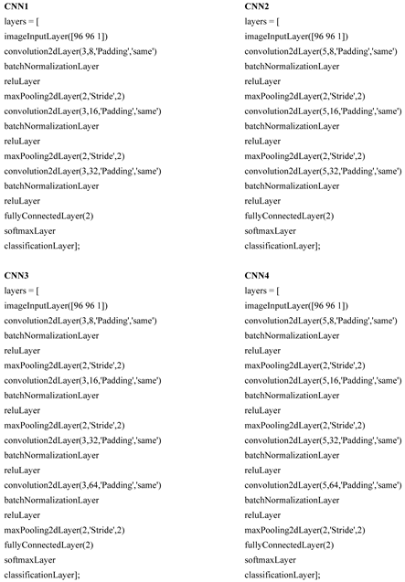
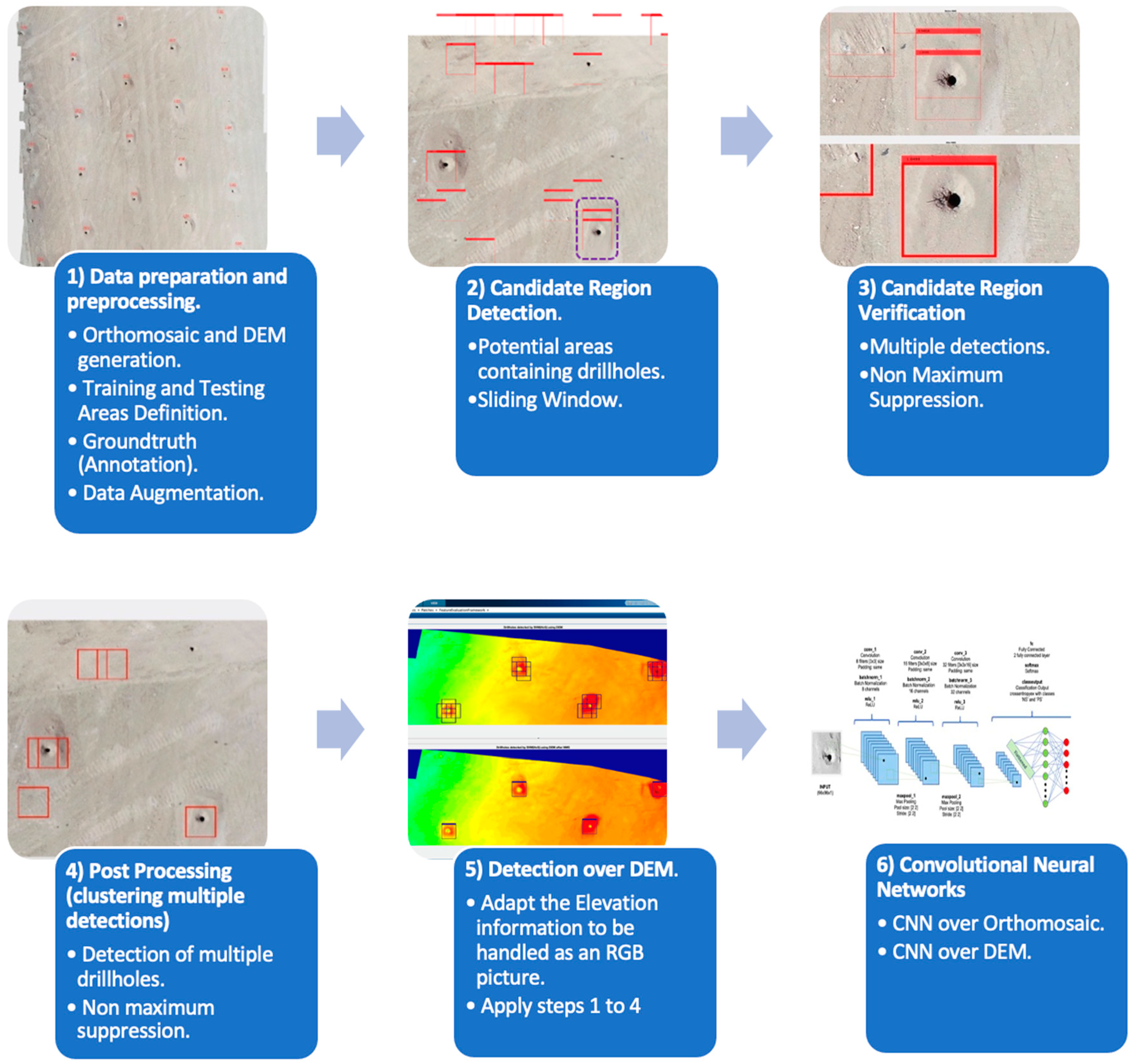
In the multiple datasets stage, the CNN-DEM framework is shown in Figure 7. The data collection for this stage was increased significantly compared to the single dataset stage (48 times more data). Optimizing essential data collection in open-pit mines in the single dataset stage laid the foundation for subsequent collection efforts, leveraging our accumulated experience. The Orthomosaic and DEM photogrammetry processing remained consistent with the single dataset stage. Blasthole annotation followed a similar process to the single dataset stage, albeit requiring additional effort and time due to the new amount of data. The data augmentation process was similar (i.e., rotations, translations, and brightness changes). The training of the CNN-DEM model was slightly different. In multiple experiments, one complete dataset was considered for testing, following a process known as Leave One Out for Cross-Validation (LOOCV). In this stage, only DEM was utilized, and the Orthomosaic of the datasets was not used. The Orthomosaics were built and used just referentially to verify the accuracy of the detections. This was necessary because, in DEM representations, it is not always easy to identify the blastholes enclosed by the bounding box detections. Four CNN architectures were used, similar to those used in the single dataset stage (Appendix B). Hyperparameter fine-tuning was time-consuming, with each run of a new set of hyperparameters requiring several hours of processing time. After obtaining low validation accuracy results using elevation values ([1469 ft–1738 ft]), the strategy was changed, and normalized elevation values ([0–1]) were employed.
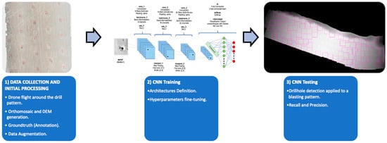
Figure 7.
Blasthole detection phases for Convolutional Neural Networks—DEM.
3.2. Data Acquisition
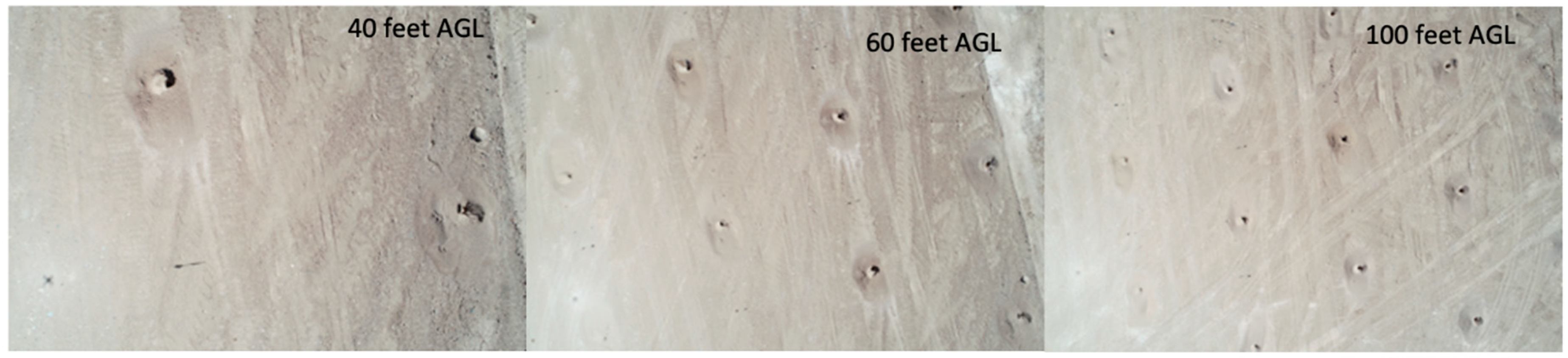
The data (drone images of blastholes in blasting patterns) were acquired in several mine sites located in Nevada, USA. The drones used in this study were a DJI Phantom 4 Pro and DJI Mavic Mini Pro. The flight options used were “manual” and “automatic”. The “manual” flight refers to capturing images using the drone’s radio controller and a generic ground control application (software app). On the other hand, “automatic” flight captures images using just a ground control application. The images were captured at different elevations above the AGL (Figure 8), e.g., 30 ft, 40 ft, 60 ft, and 100 ft, depending on the pattern size (burden × spacing).
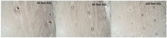
Figure 8.
Drone images of blastholes captured at 40, 60, and 100 feet.
3.3. Data Processing
3.3.1. Photogrammetry
Metashape Agisoft standard version 2.0 was the software used for the photogrammetry process. This software employed some functions, including reviewing the pictures, aligning them, building a dense cloud, constructing a mesh, and finally obtaining the Orthomosaic and DEM (Figure 9). After finishing the photogrammetry representations, patches of positive (blastholes) and negative (no-blastholes) samples were extracted from the DEM. Those patches were the inputs to build SVM and CNN models to detect blastholes.
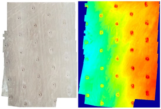
Figure 9.
Orthomosaic (left) and DEM (right) containing blastholes.
3.3.2. The Definition of Training and Testing Areas
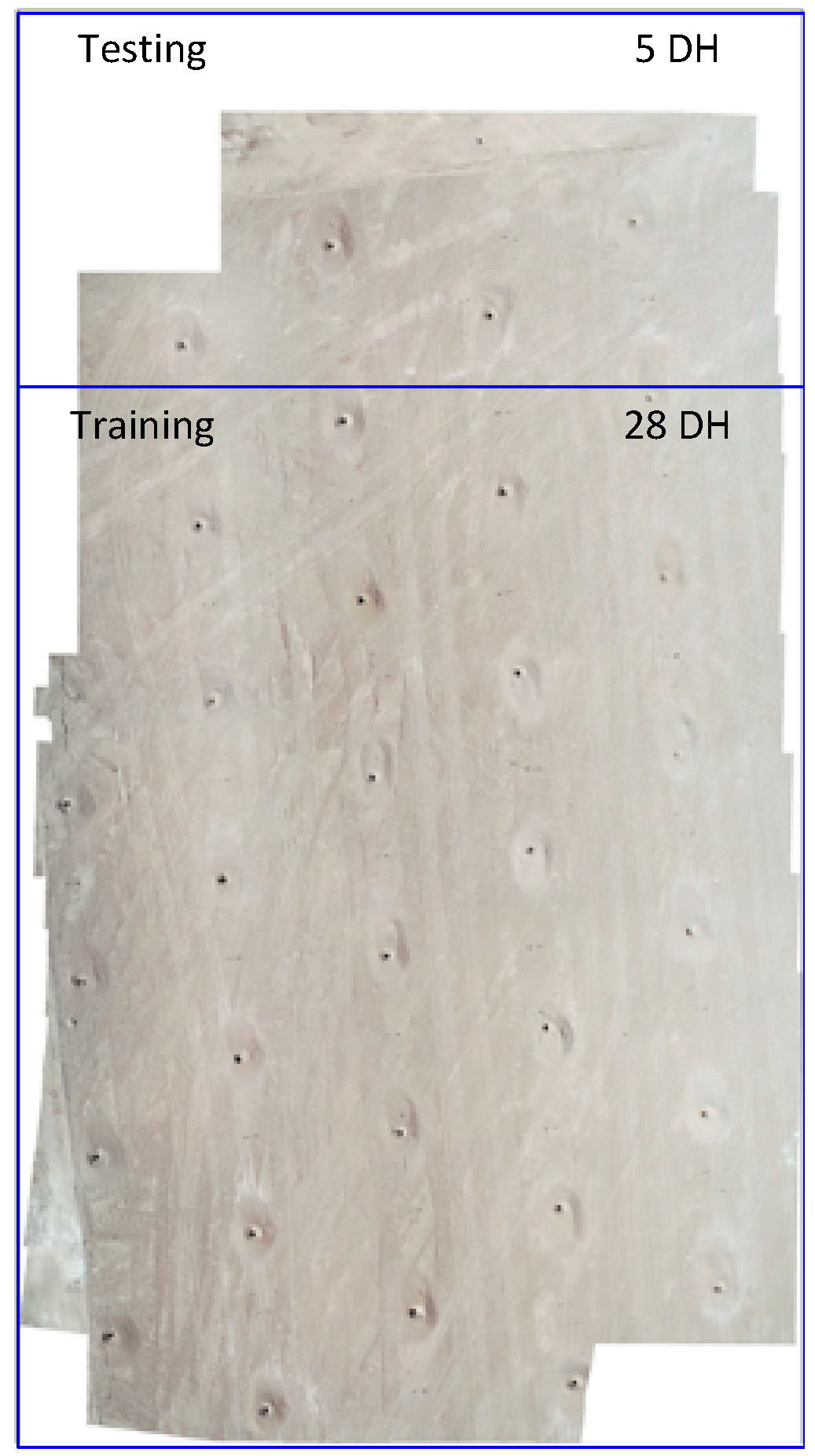
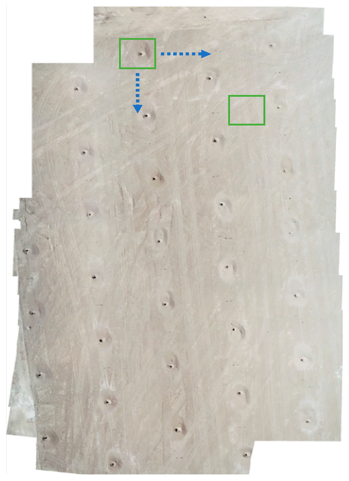
In the single dataset, the upper region of the Orthomosaic and DEM were designated as the testing area, while the lower zone was designated as the training area (Figure 10). In the case of multiple datasets, the LOOCV approach with different datasets was employed for the testing dataset, finally defining dataset number 5 for testing using normalized (0–1) elevation values.
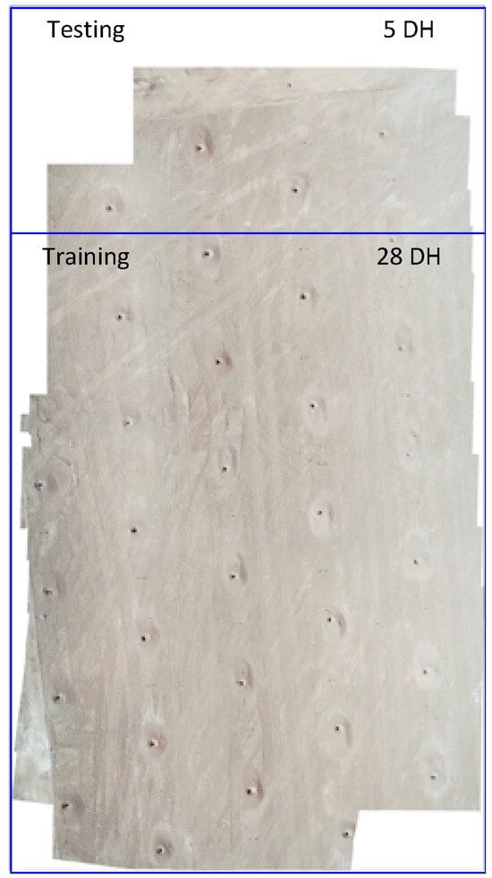
Figure 10.
Definition of training and testing areas for the single dataset.
3.3.3. Positive and Negative Samples Generation
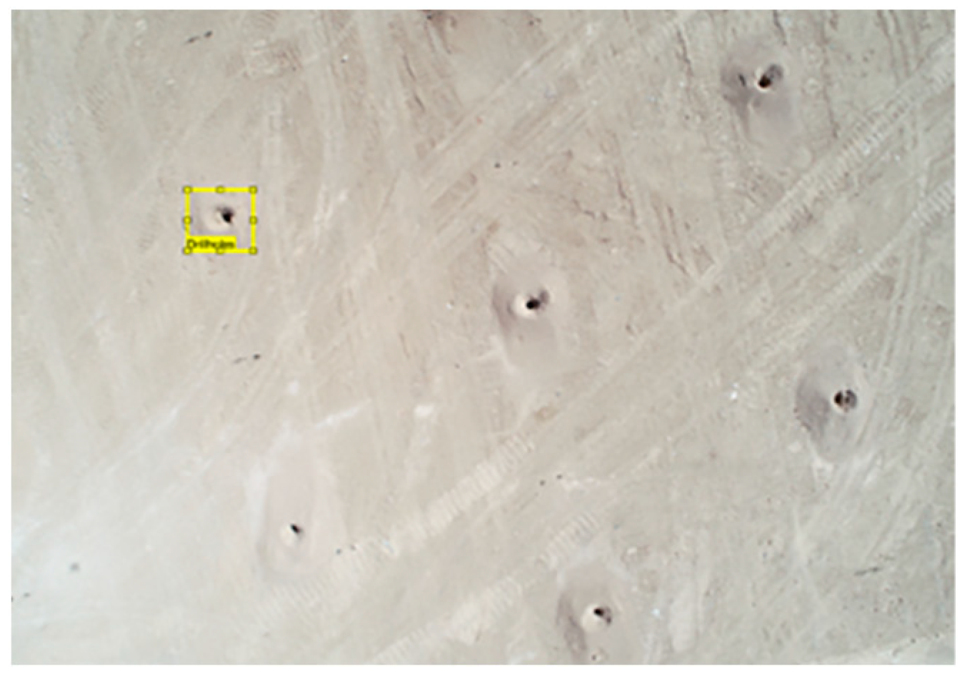
In the positive sample generation, the first step was to draw bounding boxes around the blastholes. This process is known as annotation (Figure 11). Then, the coordinates of these bounding boxes were used to extract positive sample patches from the Orthomosaic and DEM. Finally, the negative sample patches were obtained using a random sliding window algorithm, automatically extracting patches without blastholes (Figure 12).
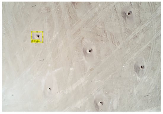
Figure 11.
Blasthole labeling (annotation) for positive sample generation.

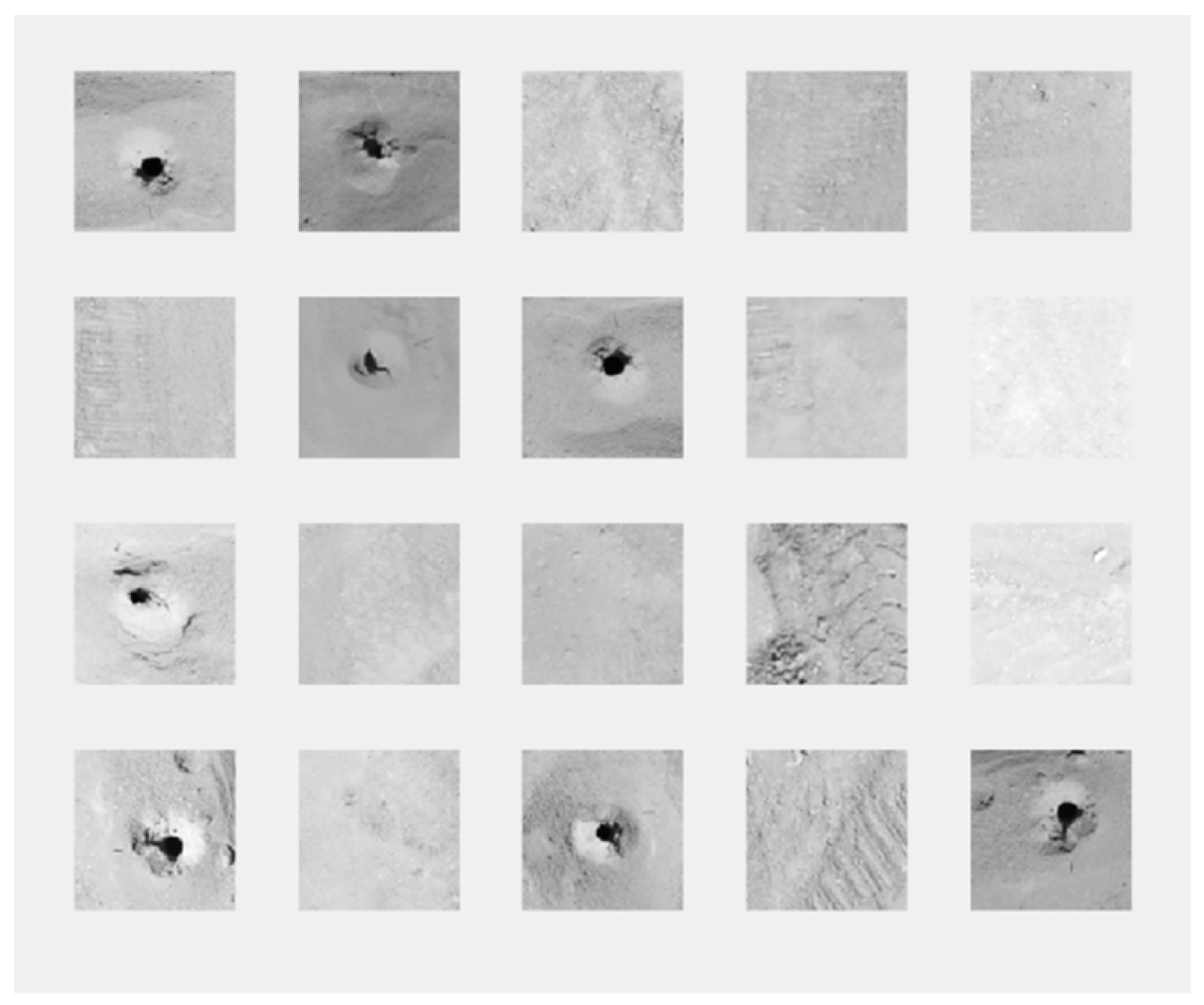
Figure 12.
Examples of positive and negative patches.
3.3.4. Sliding Window
The sliding window algorithm (Figure 13) was utilized in two different stages. The first application of the sliding window was to generate random negative sample patches. The second application of the sliding window was to divide the orthomosaic and DEM into small patches for later classification. Each of these patches was then categorized as positive or negative samples. In the case of random negative samples, the patch dimension was the average positive sample patch dimension per dataset. In the case of the sliding window to generate classification patches, the patch dimension was 300 × 300 pixels with steps of 100 pixels horizontally and vertically.
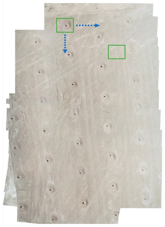
Figure 13.
Sliding Window to extract patches to be classified.
3.3.5. Data Augmentation
To provide accurate detection results, it is possible to increase the number of positive samples through a process known as data augmentation. The extracted patches are submitted to different image processing modifications, including rotations, translations, and brightness changes. The rotations of the patches were 90°, 180°, and 270° degrees. The translations were horizontal and vertical random patch locations, shifting between −30 and +30 pixels. The final stage included changes to the brightness levels of the patches between −20% and +20%. The final number of extracted positive samples is later matched with the number of negative samples via a random sliding window algorithm.
3.3.6. Training SVM
SVM training starts with creating Orthomosaic and DEM from the photogrammetry stage. Then, the positive samples (blastholes) are annotated, and the training/testing areas or datasets are defined. Afterward, a data augmentation process is used for the positive samples (blastholes). For example, a dataset is assumed to have 28 positive samples (PS). Data augmentation increases the dataset multifold due to the rotation, translation, and brightness changes. As an example, 28 PS × 4 rotations × 4 translations × 3 brightness changes at the end of the data augmentation process, resulting in 1344 PS. Next, a random sliding window algorithm was utilized to extract negative samples (NS) until reaching the same amount as the augmented positive samples. Furthermore, a HoG was used to extract features and finally obtain the SVM model.
3.3.7. Training Convolutional Neural Networks (CNN)
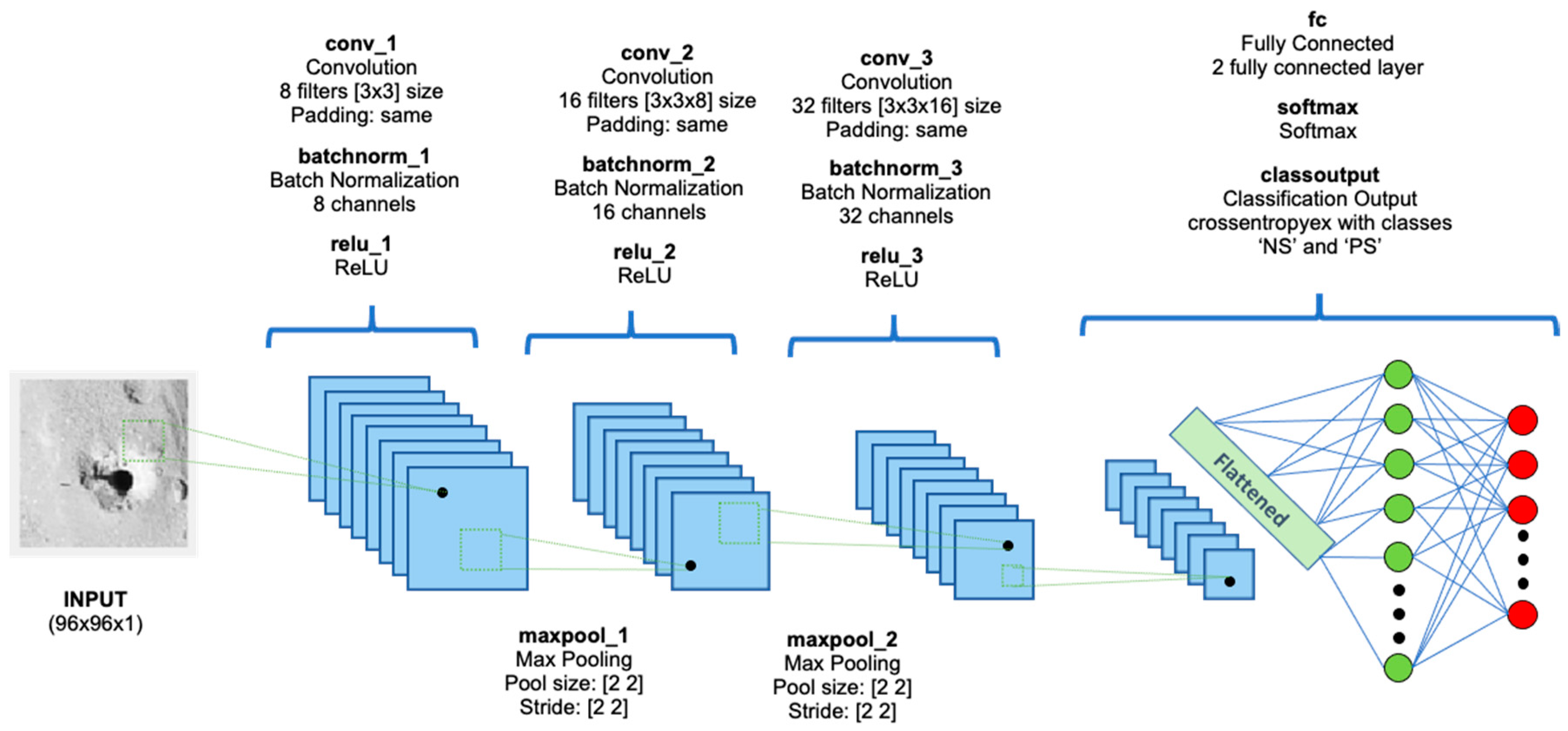
Different convolutional neural network architectures were used to detect blastholes, following the general configuration described in Figure 14, including convolution, batch normalization, max-pooling, and fully connected layers.
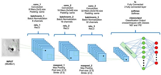
Figure 14.
CNN general architecture configuration for blasthole detection.
Every architecture (Figure 14) starts with an ImageInputLayer containing patches of 96 × 96 pixels. The processing of the patches starts with a Convolution2DLayer (CL) containing eight filters of 3 × 3 pixel size and one channel, followed by a BatchNormalization Layer (BNL) containing eight channels to normalize extreme values. The neuron activation function chosen was ReLu (Rectified Linear Unit). The link between this first block of layers and the second one corresponds to a MaxPooling2DLayer (MPL) of size 2 × 2 and stride 2 × 2. Afterward, two more similar blocks of layers were used before arriving at a FullyConnectedLayer (FCL). Finally, the outputs of the FCL were passed through a SoftmaxLayer (SL), generating the results through a ClassificationOutputLayer (COL) with two classes, corresponding to NS (no-blastholes) and PS (blastholes).
3.3.8. Testing SVM/CNN
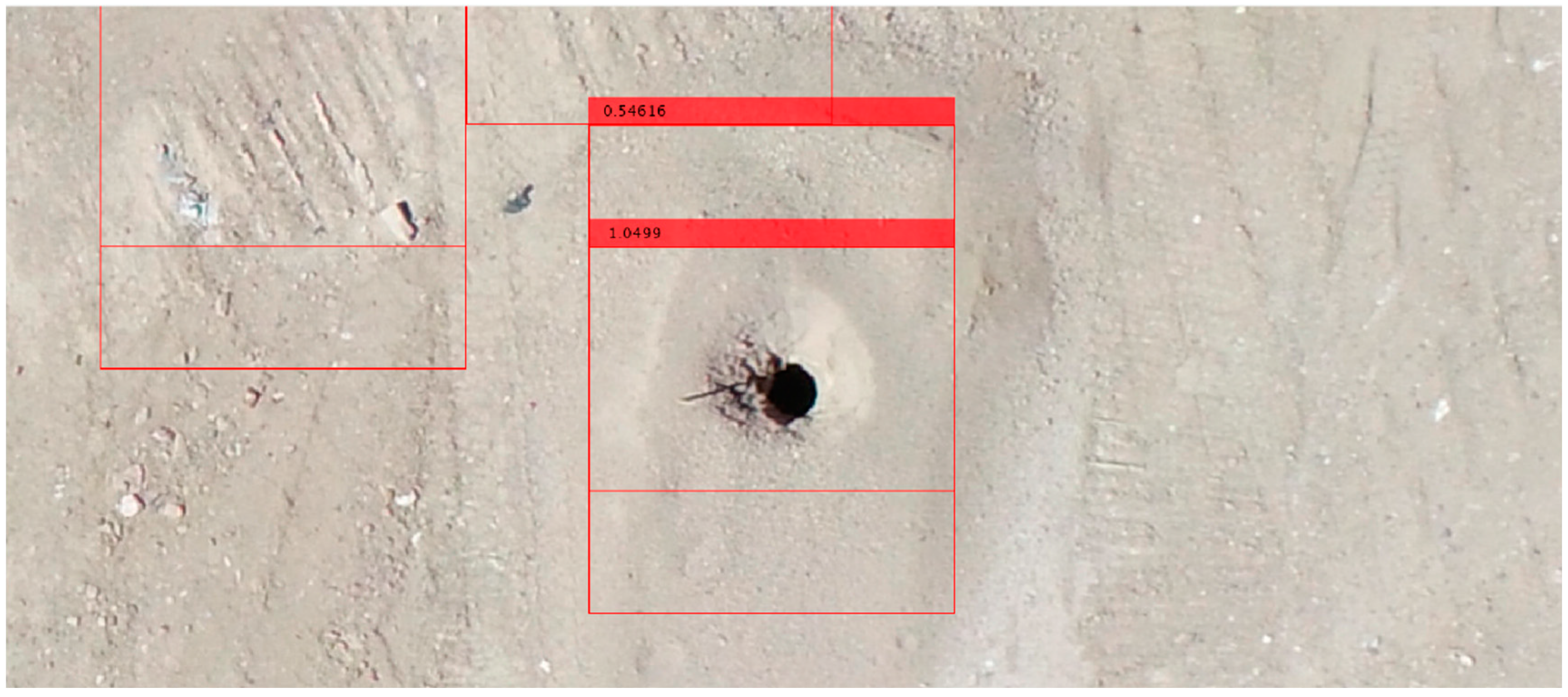
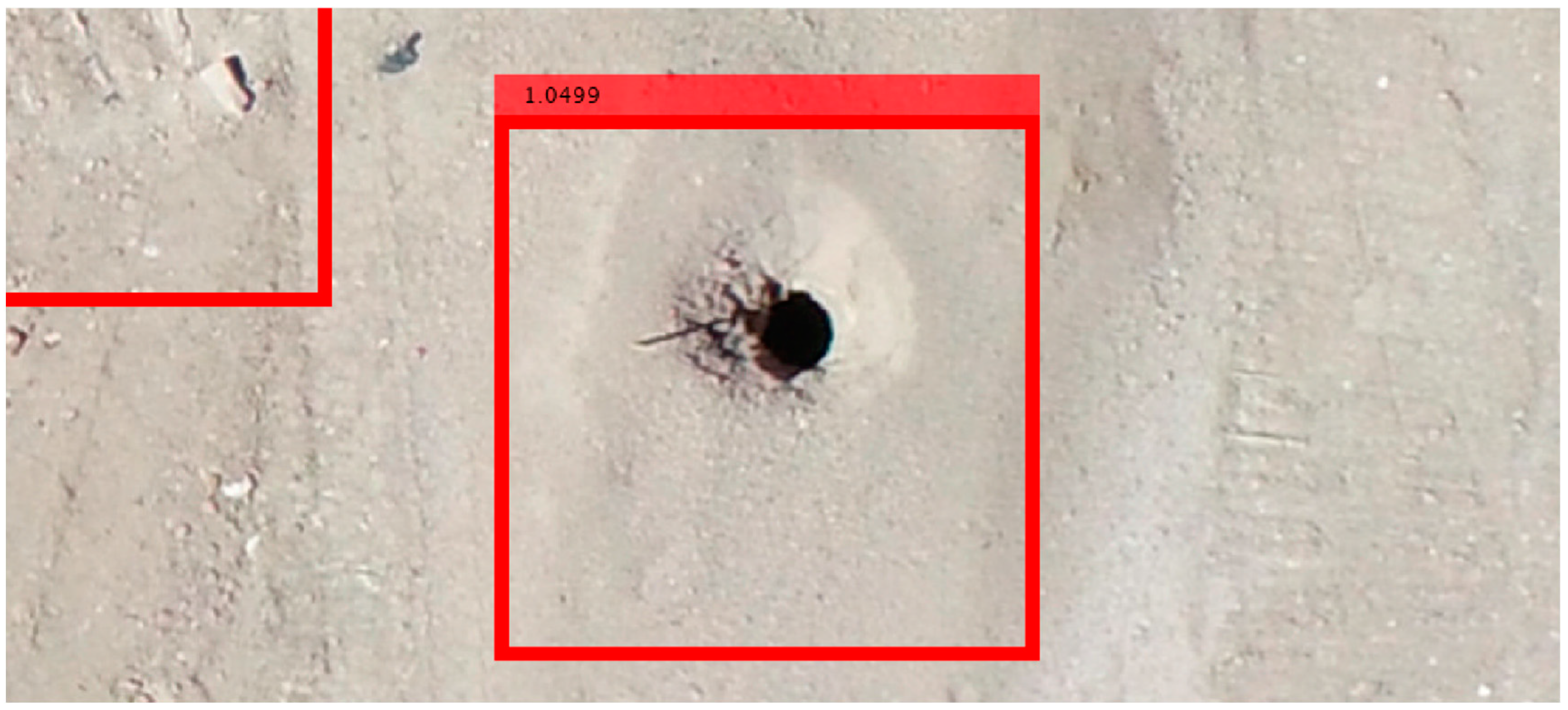
Once the training of SVM and CNN is finished, the next step is to verify (test) the detector’s accuracy. To achieve this, the “big” image (Orthomosaic and DEM) was subdivided into small patches using a sliding window algorithm. These patches are then classified as PS or NS using the SVM and CNN models (Figure 15). Finally, a non-maximum suppression method filters out the detections with the highest scores corresponding to the blastholes (Figure 16).
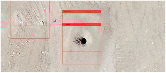
Figure 15.
Detection results before NMS with multiple bounding boxes around the blastholes.
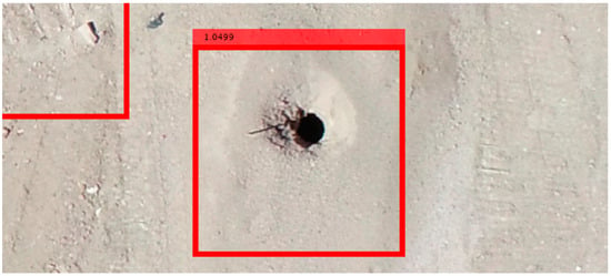
Figure 16.
Detection results after NMS keeping just the bounding box with the highest score.
4. Results and Discussion
4.1. Single Dataset
At the beginning of this study, only one single dataset was employed to develop the study framework. The dataset was divided into training and testing areas. The total number of holes in the single dataset was 33 blastholes augmented to 1344 patches through the data augmentation processes described in Section 3. This stage had three main results: SVM-Orthomosaic, SVM-DEM, and CNN-Orthomosaic.
4.1.1. SVM—Orthomosaic
The first trained model was SVM using Orthomosaic. Figure 17 illustrates the detection results in the testing area.
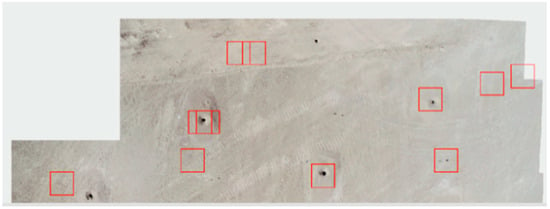
Figure 17.
SVM-Orthomosaic detection results with a single dataset.
4.1.2. SVM—DEM
The second model trained with a single dataset was SVM using DEM. Detection results are shown in Figure 18.
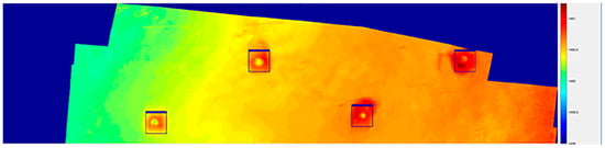
Figure 18.
SVM-DEM detection results with a single dataset.
4.1.3. CNN—Orthomosaic
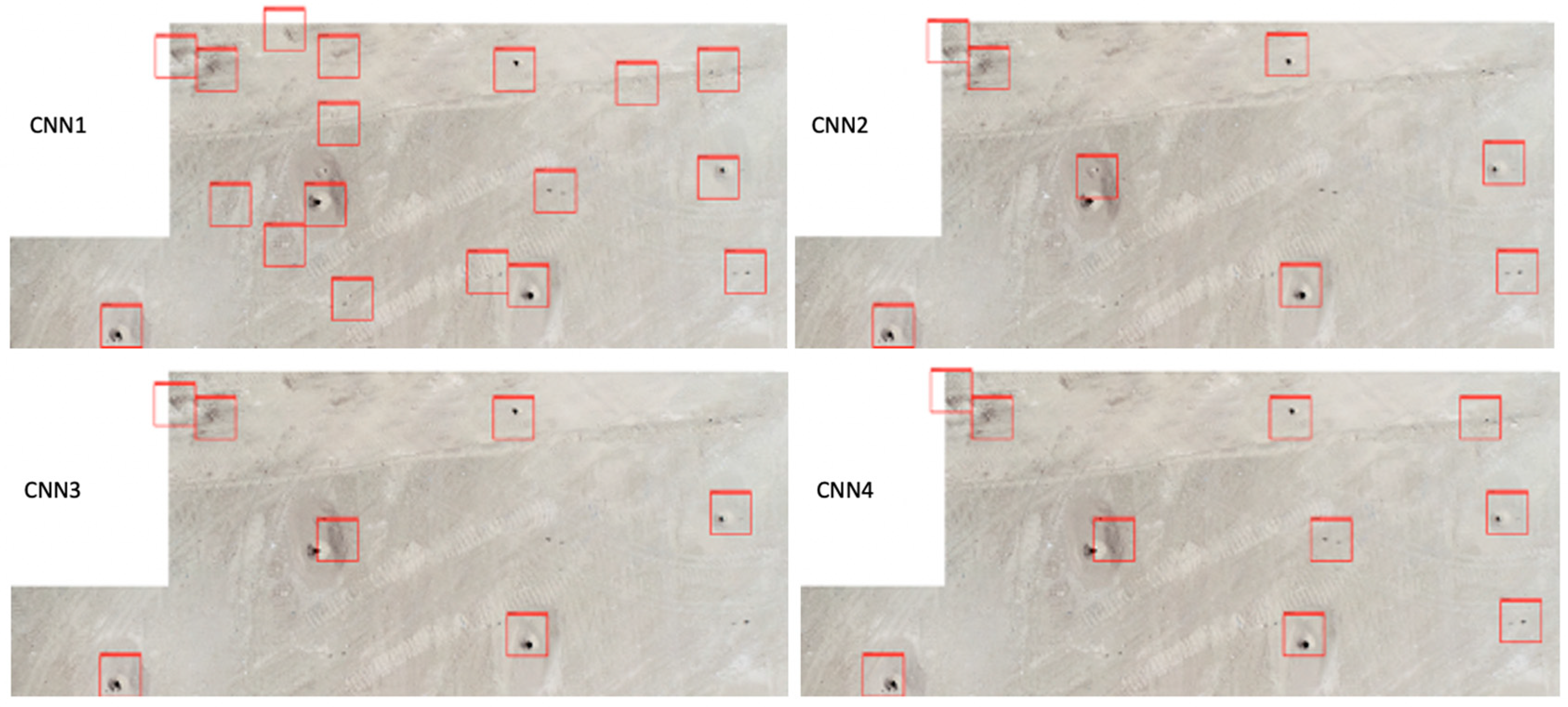
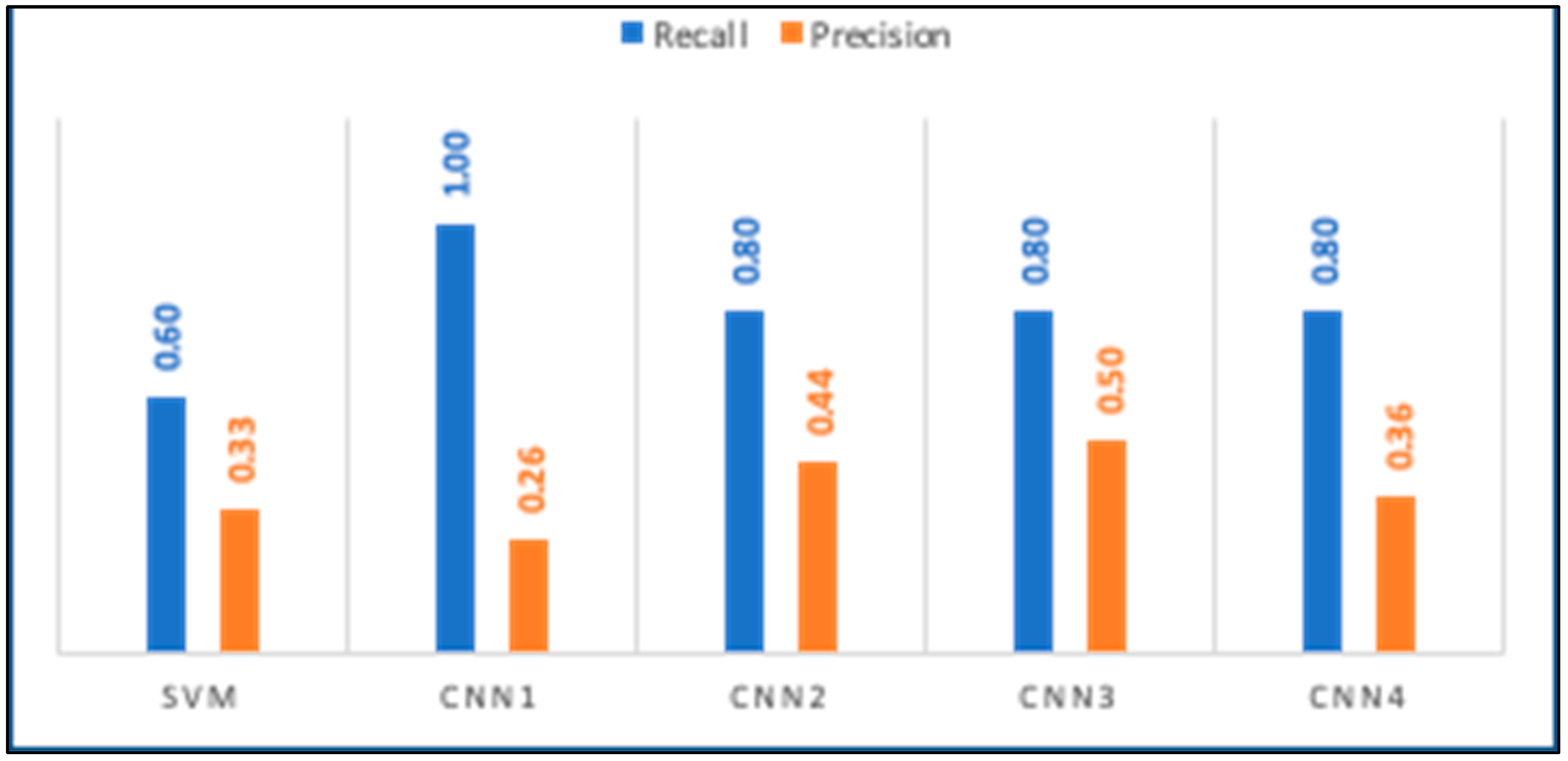
The third model trained with a single dataset utilized a Convolutional Neural Network using the Orthomosaic representation. Figure 19 indicates the detection results for the developed four CNN architectures (CNN1 through CNN4).
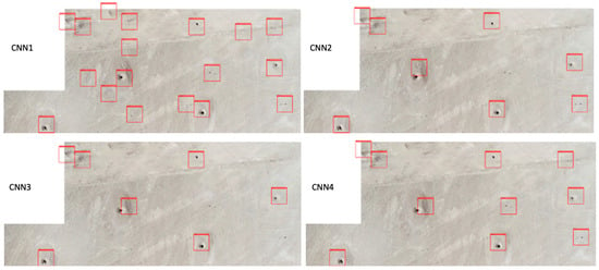
Figure 19.
CNN-Orthomosaic detection results with a single dataset.
4.1.4. Recall and Precision
In this study, two popular machine learning metrics were employed to evaluate the detection results: recall and precision. Recall (R) is defined as the number of true positives (TP) over the number of true positives plus the number of false negatives (FN) (Equation (8)) [41].
Precision (P) is formulated as the number of true positives (TP) over the number of true positives plus the number of false positives (FP) (Equation (9)) [41].
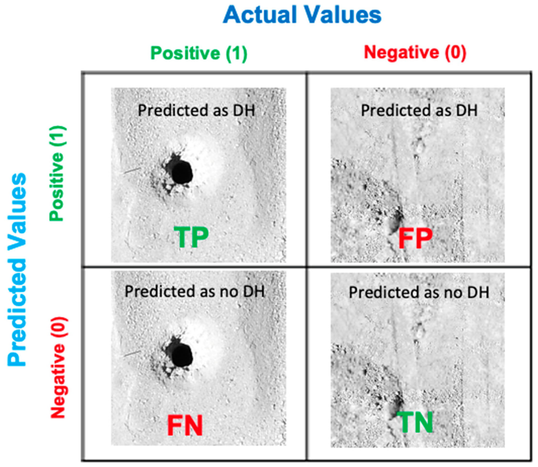
The recall and precision have been calculated using the confusion matrix (Figure 20). The key definitions to estimate the confusion matrix are as follows:
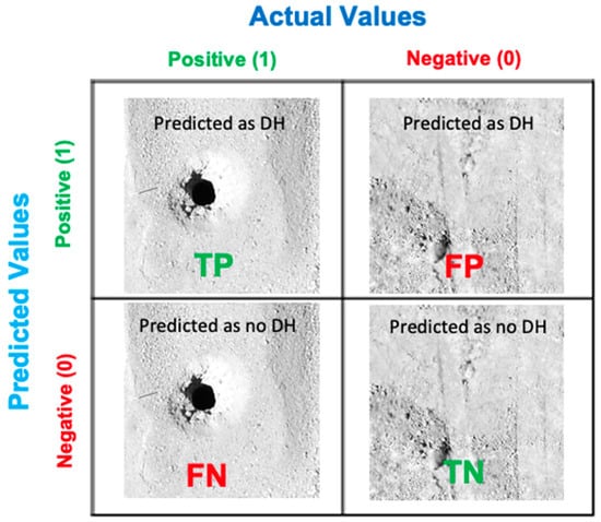
Figure 20.
Confusion Matrix for blasthole detection (DH: Blasthole).
- -
- True Positive (TP): Predicted as blasthole when it is a blasthole.
- -
- True Negative (TN): Predicted as no-blasthole when it is not a blasthole.
- -
- False Positive (FP): Predicted as blasthole, but it is not a blasthole.
- -
- False Negative (FN): Predicted as no-blasthole, but it is a blasthole.
Finally, several detections around the blastholes were filtered out using the non-maximum suppression algorithm, keeping just the detection with the highest score in each case.
Recall and precision (Table 1) were used to compare the results of SVM and CNN detection. Figure 21 displays recall and precision for the five models built (1 SVM, 4 CNN) using the Orthomosaic. The best results were obtained using CNN. Also, in the comparison of detection results between Orthomosaic and DEM (Figure 17 and Figure 18), DEM demonstrated superior performance. For these reasons, the authors have chosen to proceed to the next stage, utilizing CNN and DEM with multiple datasets.

Table 1.
Recall and Precision Results before and after NMS (TP: True Positives, FP: False Positives, FN: False Negatives).
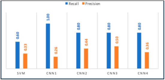
Figure 21.
Recall and Precision results using the Orthomosaic for SVM and CNN.
4.2. Multiple Datasets
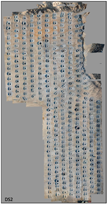
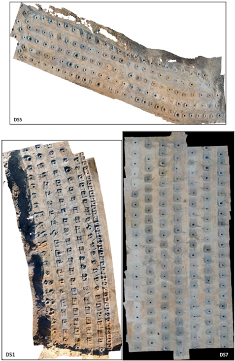
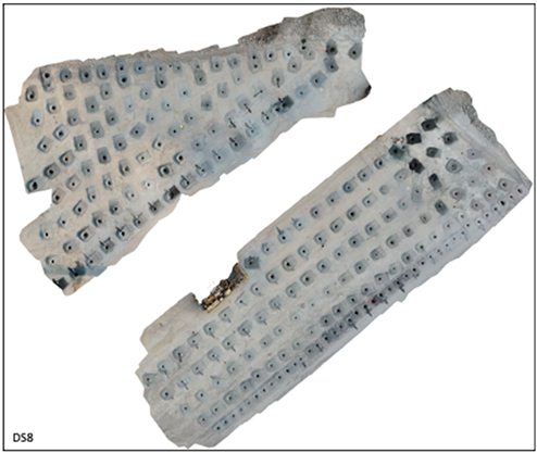
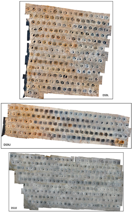
Based on the single dataset results, this study focused on applying CNN with DEM at this stage. Appendix A provides the Orthomosaics for the datasets used in this stage. In this phase, the quantity of collected data exponentially increased from 33 to 1573 blastholes. This increase means 48 times the initial dataset. Table 2 provides a detailed description of the number of blastholes captured for each dataset. After data augmentation, the total number of patches involved in the training/testing process was 11,007 patches.
Table 2.
The number of holes and patches for each dataset.
CNN—DEM
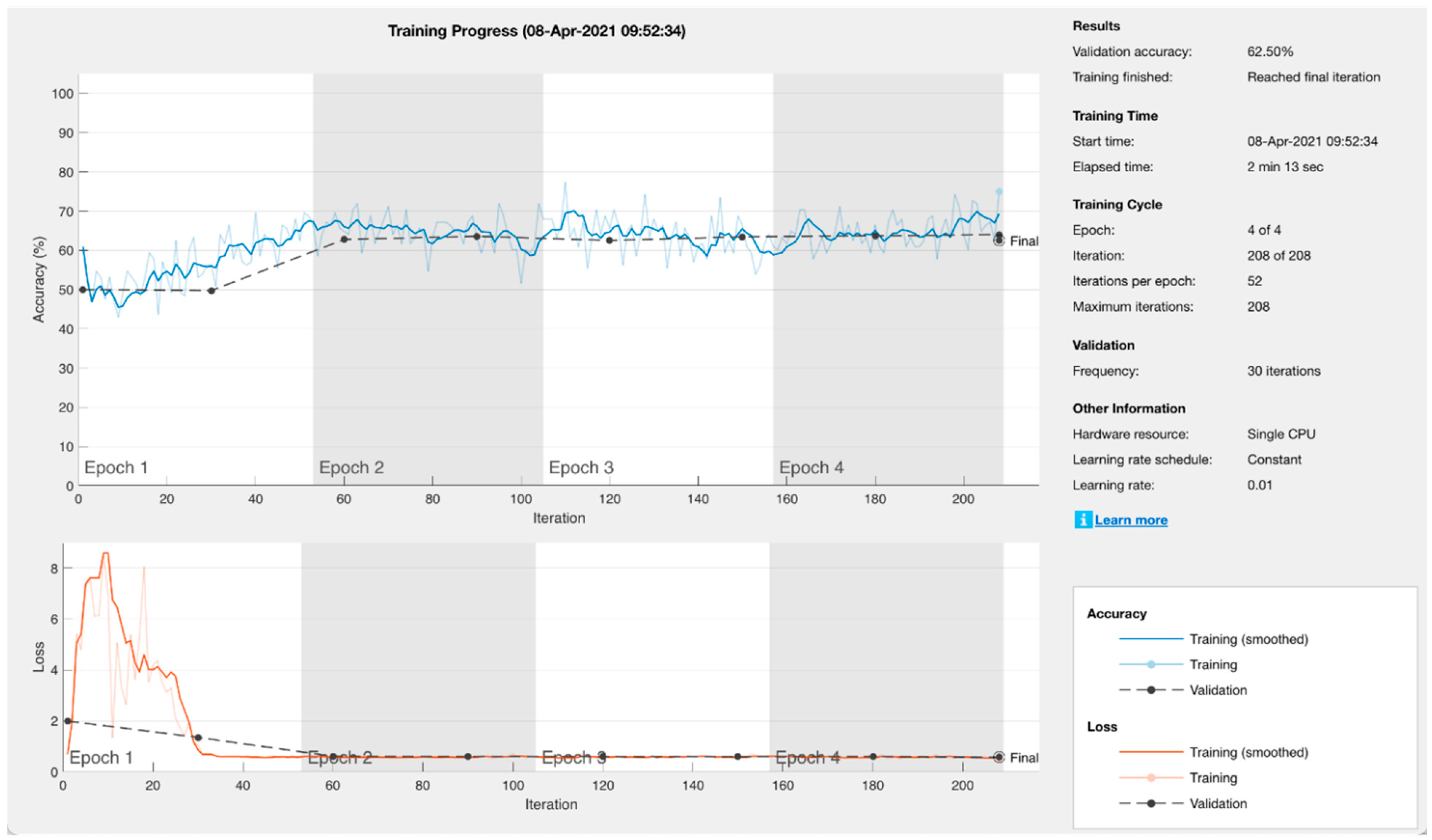
In this stage, Convolutional Neural Networks on DEM with seven datasets were employed for training, and one complete dataset was utilized for testing. Also, multiple experiments were performed with different elevation values. The first experiment used LOOCV, but the validation accuracy was around 60% (Figure 22). In addition, some LOOCV combinations generated just negative sample results. The second experiment was to group datasets with similar elevations for training and testing, but the validation accuracies were between 70% and 80%. Finally, the third group of experiments was performed by normalizing the elevation values, obtaining validation accuracy results greater than 90%. Detection results using normalized elevation values and the testing dataset DS5 are shown in Figure 23 and Figure 24. These results can be verified using the results provided in Table 3, which outlines the detection results for normalized elevation values. The table includes several columns, including the number of layers, experiment numbers E1 through E5, proportions of training and testing data, learning rate used in each experiment, epochs used in the experiments, the number of detected holes after non-maximum suppression, and the last column gives the percentage of detected holes in each experiment. In this case, the testing dataset was DS5, containing 139 blastholes. The best experiment, achieved by E5, detected all the blastholes in the testing dataset. The combination of normalized elevation values, increased training data, and optimized learning rate contributed to the superior performance of Experiment 5 in accurately detecting blastholes. These adjustments demonstrate the importance of thorough experimentation and parameter tuning in achieving optimal results in machine learning tasks.
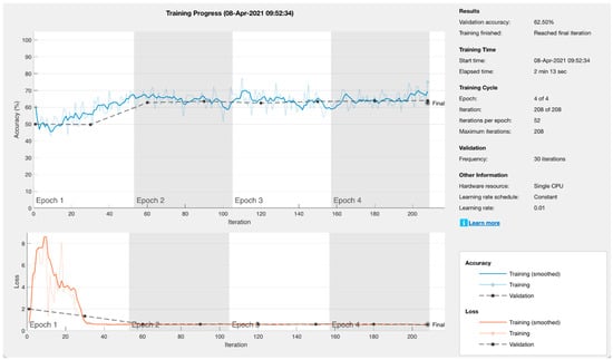
Figure 22.
Training progress screen with a validation accuracy of 62.5%.
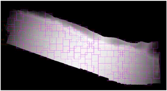
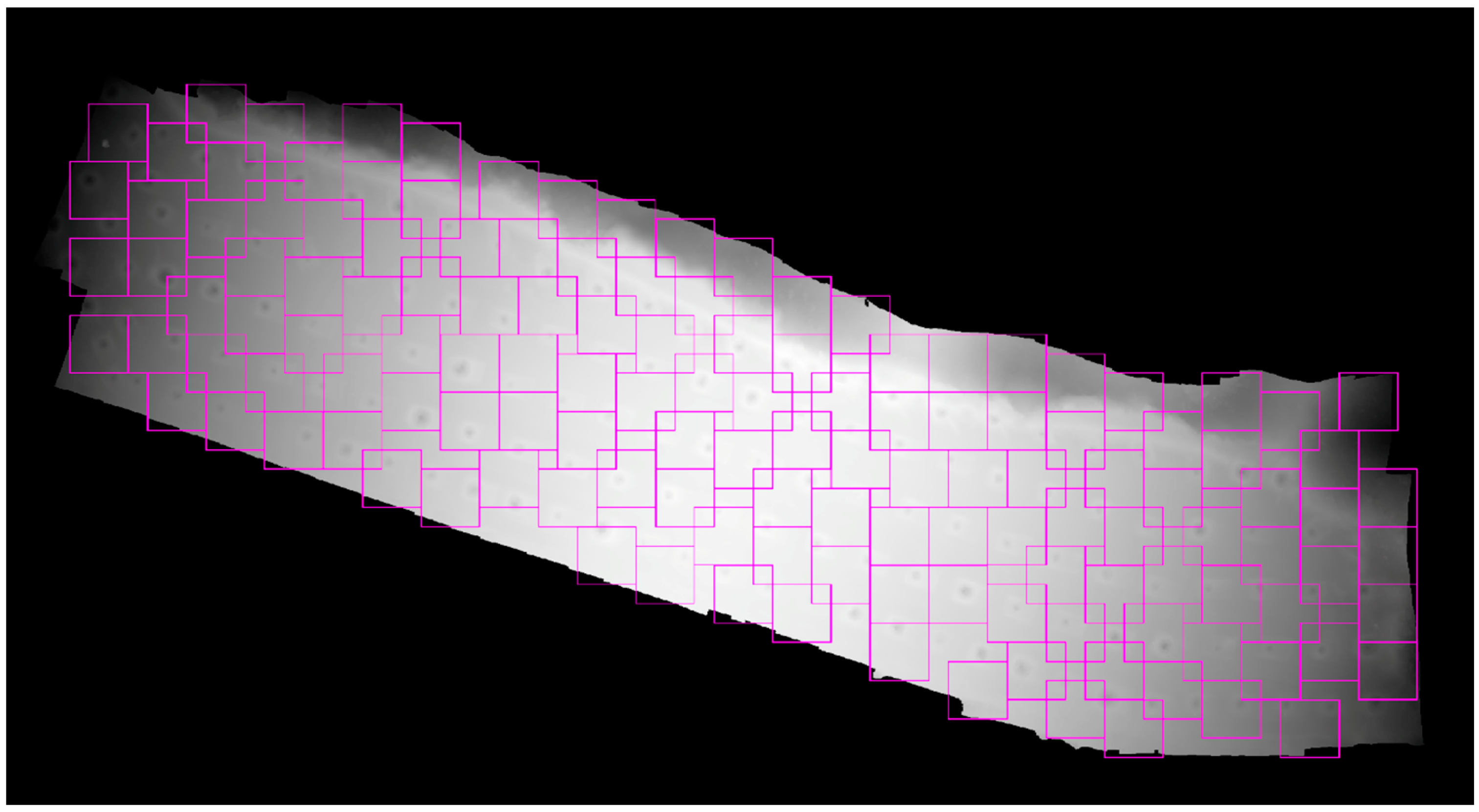
Figure 23.
Detection results with bounding boxes displayed over the testing dataset (DEM).

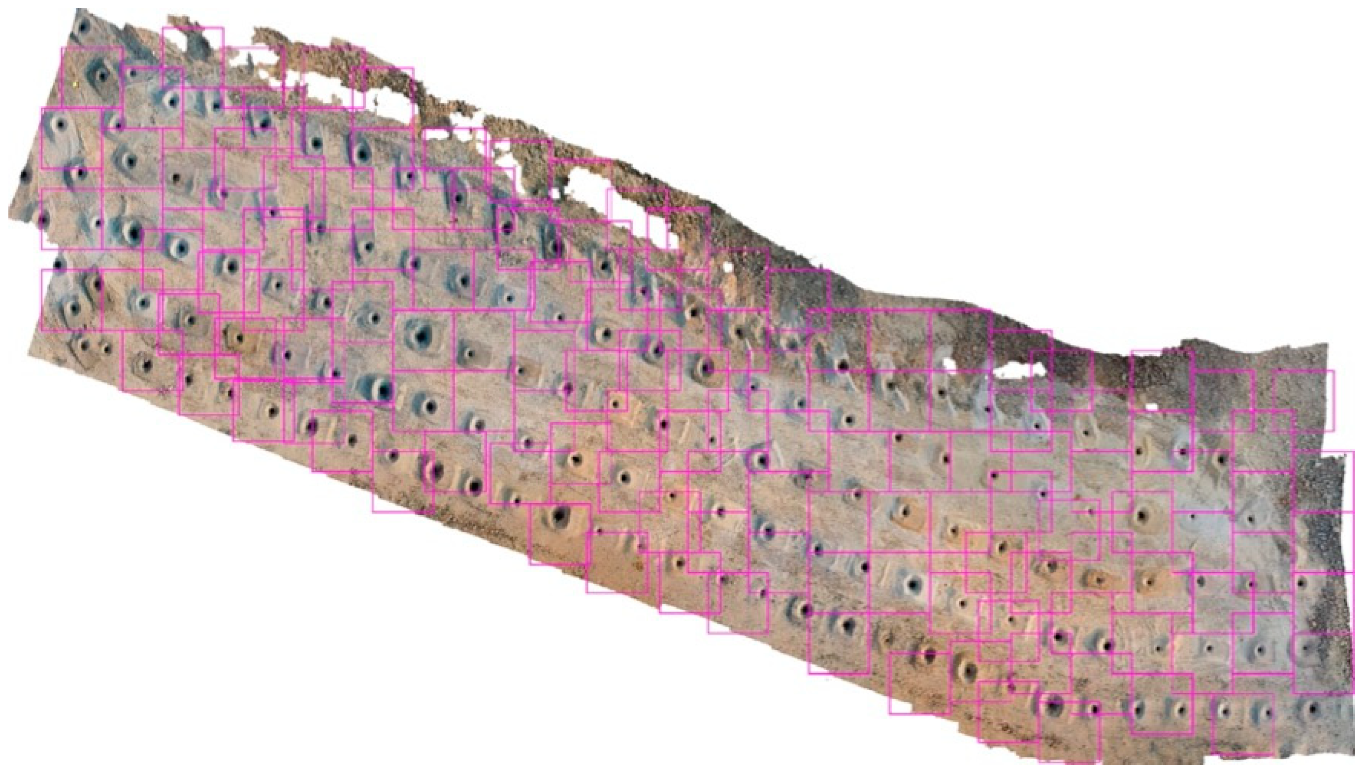
Figure 24.
Detection results with bounding boxes are displayed over the testing dataset (Orthomosaic).
Table 3.
Experiment results using normalized elevation values and DS5 as the testing dataset.
Furthermore, for blasthole detection purposes, the percentage of detected holes is a more representative metric than recall and precision typically used in machine learning.
4.3. Performance Analysis of All Experiments
Many studies indicate that achieving a high recall value or precision is dependent on the specific application. The objective of this study is clear: to detect as many blastholes as possible. This section examines the performance results of the models developed throughout the study.
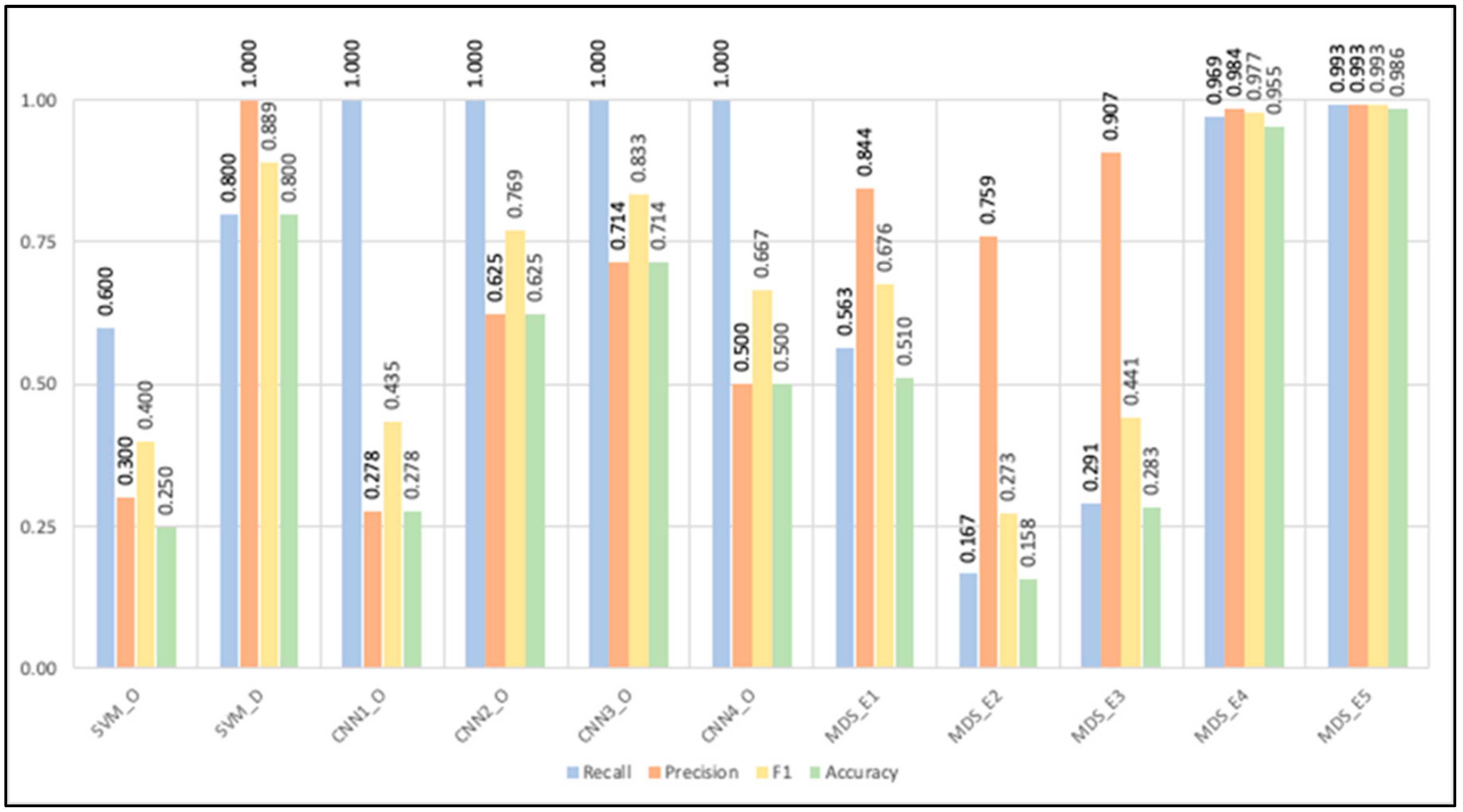
Figure 25 illustrates four performance indicators that were evaluated and compared: recall, also known as sensitivity, precision, F1 score, and accuracy. The recall represents the proportion of correctly predicted blastholes out of all the blastholes in the pattern. Precision is the percentage of detections (bounding boxes) that were accurate. The F1 score is the harmonic mean of recall and precision. Accuracy measures how effectively the model considers both positive and negative cases.
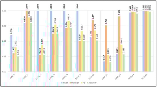
Figure 25.
Performance results of the eleven models built during the research.
As depicted in Figure 25, the first model (SVM_O = SVM_Orthomosaic) exhibits low-performance metrics. In the second model (SVM_D = SVM_DEM), a significant improvement is observed in the metric scores compared to the first model, attributed to using Digital Elevation Maps (DEMs) for detections. CNN architectures were employed for the subsequent four groups of bars (CNN1_O, CNN2_O, CNN3_O, and CNN4_O) to achieve better performance results, particularly for CNN number 3 (CNN3_O), which stood out. Subsequently, we transitioned to the “multiple dataset stage”, where the first three rounds of experiments initially showed low-performance results (MDS_E1, MDS_E2, MDS_E3). However, the score results for experiment E4 (MDS_E4) demonstrated a significant improvement, while experiment E5 yielded outstanding results.
Furthermore, upon analyzing Figure 25 and commencing with the single dataset stage, models built using SVM and DEM (recall: 0.80, precision: 1.0, F1: 0.89, and accuracy: 0.89) outperformed those built using SVM with Orthomosaic (recall: 0.6, precision: 0.3, F1: 0.4, and accuracy: 0.25). Hence, we opted for DEM and CNNs in the final phase of the study, the multiple dataset stage, where we achieved remarkable recall, precision, F1, and accuracy values of 0.99. These high-performance values are not typical in other blasthole detection studies, as evidenced by comparisons with prior literature. For instance, in a study by [9], they obtained a recall of 0.423 and a precision of 0.7115 without reporting the F1 score. Conversely, Zhang et al. [10] utilized IoU and Dice to evaluate models based on semantic segmentation. After the multiple datasets stage, our detectors successfully identified most blastholes in the drill pattern, with just one hole missed, demonstrating the excellent performance of the developed models. These outstanding results were attained through experimentation with different modeling alternatives.
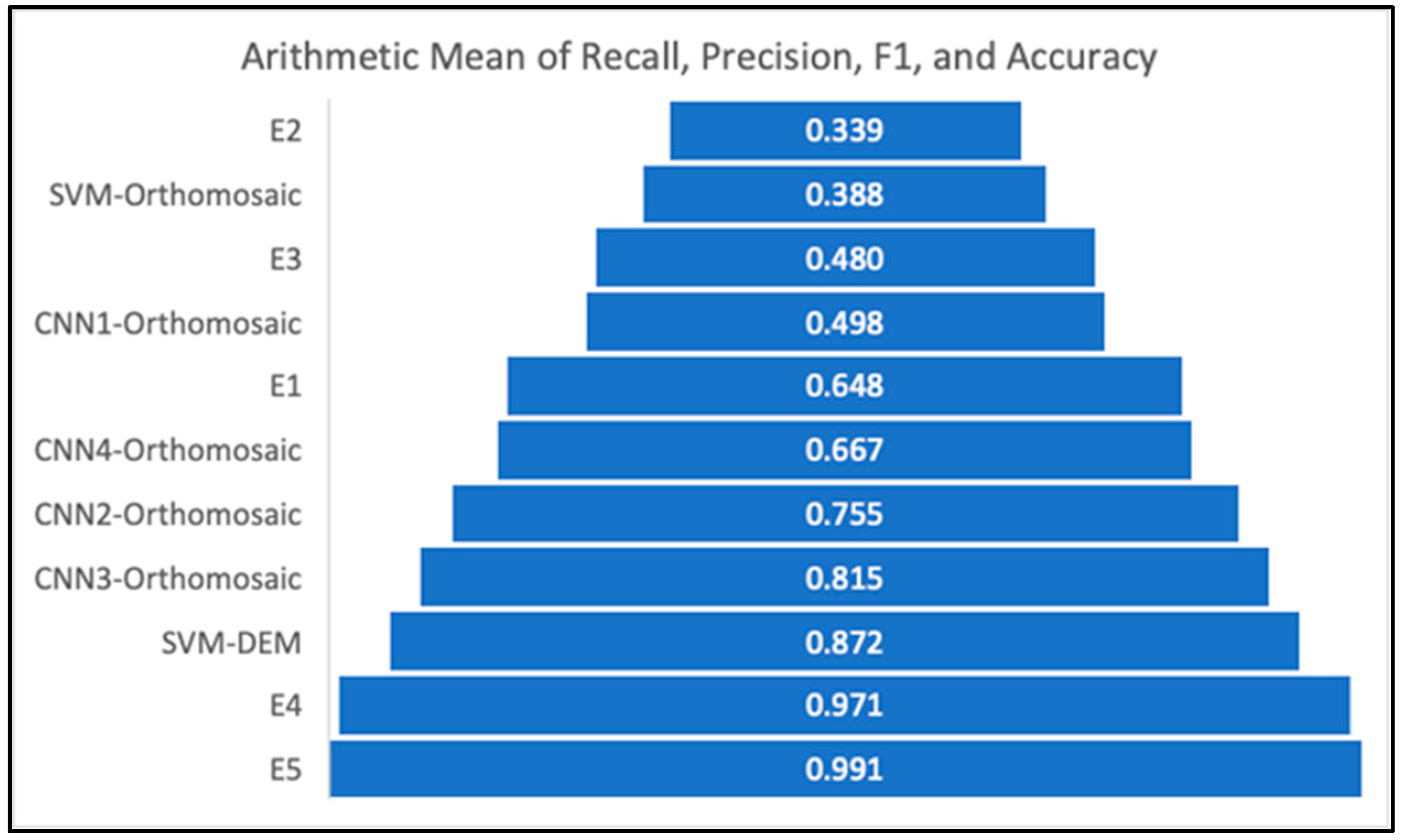
Seeking to summarize the performance results in a single metric, we calculated the arithmetic and harmonic mean of recall, precision, F1, and accuracy (Figure 26 and Figure 27). This method effectively sorted the models based on their overall performances. The clear winner was experiment E5 of the multiple dataset stage, with a harmonic mean (H) of 0.991, closely followed by experiment E4 with H = 0.971. SVM-DEM (H = 0.865) secured the third position, while the CNN3-Orthomosaic model (H = 0.8) ranked fourth.

Figure 26.
The arithmetic mean of performance metrics considers recall, precision, F1, and accuracy.
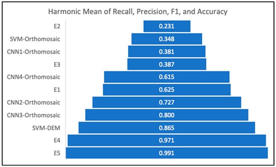
Figure 27.
The harmonic mean of performance metrics considers recall, precision, F1, and accuracy.
4.4. Detection of Snow-Covered Drill Holes Using CNN
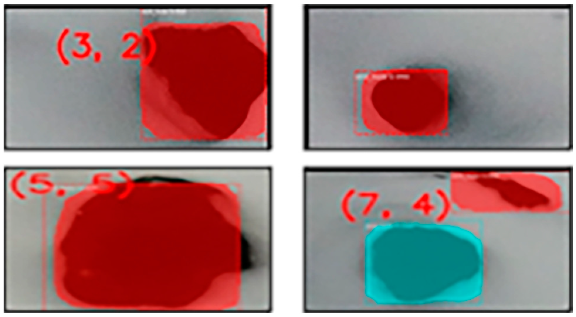
The winter season in Nevada is characterized by snowfall within the region, covering the blastholes with snow. To detect these snowy holes, a new CNN model was developed using a Mask R-CNN (Region-Based Convolutional Neural Networks) architecture (Figure 28). The Mask R-CNN is an object detection model based on a deep CNN architecture developed by researchers in 2017. Mask R-CNN provided high accuracy in object detection problems. The model development procedure was comparable to the steps detailed previously in this paper. The model returns a bounding box and a mask for each detected object. In this case, 90% and 10% of the data were used for training/validation and testing, respectively. The tool used for the annotation stage was VIA (VGG Image Annotator). VIA converts the annotation process to a JSON file specifying the bounding boxes’ extent and coordinates.
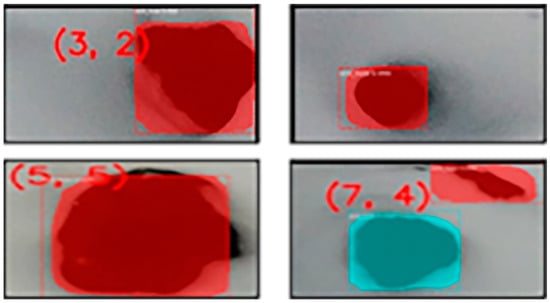
Figure 28.
Snow-covered blastholes detected by the Mask R-CNN Model.
5. Conclusions
The following conclusions can be derived from this research work:
- Blasthole detection using drones and machine learning aims to be a complementary or supplementary way to identify the ultimate location of blastholes and improve the distribution of explosive energy in the blasting process.
- The proposed solution in this study can be used in open-pit mines for drilling accuracy control, enabling drill and blast engineers to simulate and adjust blasting parameters, optimizing blasting results, and improving the safety of the process.
- The research offers a new way to control the drilling accuracy in open-pit mines (not just surveys and GPS mounted over the drill rigs).
- The experiment results demonstrated that it could be possible to automatically detect blastholes on aerial images (captured through a drone) under different seasonal conditions, using Support Vector Machine and Convolutional Neural Networks in open-pit mines.
- The proposed solution provides a way to control drilling accuracy deviations in blast patterns. These inaccuracies occur for several reasons: signal loss in certain mine areas (known as blind spots), operational factors such as drilling near pit edges, or overbreaking resulting from previously blasted patterns.
- Another potential application of this research is to define the extension of the polygon blasted for ore control purposes.
- With a single dataset, detection results using SVM over DEM yielded better results than SVM with Orthomosaic representations, but the best results for the single dataset were obtained using Convolutional Neural Networks and Orthomosaic.
- In the case of multiple datasets, the most favorable results were obtained in experiment E5, wherein all 139 blastholes were detected. This process was accomplished using normalized elevation values and specific hyperparameters: 81% of the data for training, 19% for testing, a learning rate of 0.1, and 4 epochs.
- Hyperparameter tuning was the most time-consuming activity during the training of the CNN-DEM architectures because of the high amount of information in the datasets.
- In this machine learning application, prioritizing the detection of blastholes, the percentage of detected holes proves to be a more representative metric compared to the conventional recall and precision metrics. The final goal of the study is to identify as many blastholes as possible.
- In this study, the percentage of detected holes was the best performance metric. This issue differs from typical deep learning applications in computer vision, where recall and precision are commonly used as performance metrics.
- Future work will involve collecting data from various mine sites encompassing different rock formations, drilling diameters, and weather conditions to develop models capable of detecting blastholes across diverse environments.
- Additionally, exploring the utility of the images captured for blasthole detection for other applications, such as delineating blasting overbreak and estimating the volume and tonnage of blast patterns, presents an avenue for further research and application.
Author Contributions
Conceptualization, J.S.; Methodology, E.E. and R.B.; Software, J.V. and A.J.; Investigation, J.V., E.E., R.B. and A.J.; Resources, J.S.; Data curation, E.E. and A.J.; Writing—original draft, J.V.; Writing—review & editing, J.A.G. and A.M.-M.; Supervision, J.S.; Project administration, J.S. All authors have read and agreed to the published version of the manuscript.
Funding
This study is a part of the project supported by the Center for Disease Control and Prevention and the National Institute for Occupational Health and Safety under contract number 75D30119C06044.
Institutional Review Board Statement
Not applicable.
Informed Consent Statement
Not applicable.
Data Availability Statement
Data are contained within the article.
Acknowledgments
The authors are responsible for this project’s recommendations, conclusions, and findings. The outcomes do not necessarily reflect the views of the National Science Foundation, the Center for Disease Control and Prevention, or the National Institute for Occupational Health and Safety.
Conflicts of Interest
The authors declare no conflicts of interest.
Appendix A. Datasets
Appendix B. CNN Networks
References
- Bamford, T.; Medinac, F.; Esmaeili, K. Continuous monitoring and improvement of the blasting process in open pit mines using unmanned aerial vehicle techniques. Remote Sens. 2020, 12, 2801. [Google Scholar] [CrossRef]
- Girard, J.M.; McHugh, E. Detecting Problems with Mine Slope Stability. In Proceedings of the Thirty-First Annual Institute on Mining Health, Safety and Research, Roanoke, VA, USA, 27–30 August 2000. [Google Scholar]
- Kamran-Pishhesari, A.; Moniri-Morad, A.; Sattarvand, J. Applications of 3D Reconstruction in Virtual Reality-Based Teleoperation: A Review in the Mining Industry. Technologies 2024, 12, 40. [Google Scholar] [CrossRef]
- Marsh, E.; Dahl, J.; Kamran Pishhesari, A.; Sattarvand, J.; Harris, F.C., Jr. A Virtual Reality Mining Training Simulator for Proximity Detection. In Proceedings of the International Conference on Information Technology-New Generations, Las Vegas, NV, USA, 24 April 2023; pp. 387–393. [Google Scholar]
- A Step Change in Mining Productivity|AusIMM Bulletin. 2015. Available online: https://search.informit.org/doi/abs/10.3316/ielapa.156763317610968 (accessed on 10 July 2021).
- GPS.gov: GPS Accuracy. (n.d.). Available online: https://www.gps.gov/systems/gps/performance/accuracy/ (accessed on 11 July 2022).
- de Ingeniería, F.; Patricio Valencia López Profesor Guía, J.; Humberto Contreras Moreno, E. Evaluación de Alternativas de Perforación y Tronadura Para el Mejoramiento de la Fragmentación; Mina Los Filos: Estado de Guerrero, México, 2015. [Google Scholar]
- The Hole Story: The Benefits of Drill and Blast|Engineer Live. (n.d.). Available online: https://www.engineerlive.com/content/hole-story-benefits-drill-and-blast (accessed on 10 July 2022).
- Pan, S.; Tian, Z.; Qin, Y.; Yue, Z.; Yu, T. Intelligent Blasthole Detection of Roadway Working Face Based on Improved YOLOv7 Network. Appl. Sci. 2023, 13, 6587. [Google Scholar] [CrossRef]
- Zhang, Z.; Deng, H.; Liu, Y.; Xu, Q.; Liu, G. A Semi-Supervised Semantic Segmentation Method for Blast-Hole Detection. Symmetry 2022, 14, 653. [Google Scholar] [CrossRef]
- Arthur, C.K.; Temeng, V.A.; Ziggah, Y.Y. Soft computing-based technique as a predictive tool to estimate blast-induced ground vibration. J. Sustain. Min. 2019, 18, 287–296. [Google Scholar] [CrossRef]
- Azimi, Y.; Khoshrou, S.H.; Osanloo, M. Prediction of blast induced ground vibration (BIGV) of quarry mining using hybrid genetic algorithm optimized artificial neural network. Measurement 2019, 147, 106874. [Google Scholar] [CrossRef]
- Dong, L.; Li, X.; Xu, M.; Li, Q. Comparisons of Random Forest and Support Vector Machine for Predicting Blasting Vibration Characteristic Parameters. Procedia Eng. 2011, 26, 1772–1781. [Google Scholar] [CrossRef]
- Hajihassani, M.; Jahed Armaghani, D.; Sohaei, H.; Tonnizam Mohamad, E.; Marto, A. Prediction of airblast-overpressure induced by blasting using a hybrid artificial neural network and particle swarm optimization. Appl. Acoust. 2014, 80, 57–67. [Google Scholar] [CrossRef]
- Hasanipanah, M.; Monjezi, M.; Shahnazar, A.; Jahed Armaghani, D.; Farazmand, A. Feasibility of indirect determination of blast induced ground vibration based on support vector machine. Measurement 2015, 75, 289–297. [Google Scholar] [CrossRef]
- Khandelwal, M.; Kankar, P.K.; Harsha, S.P. Evaluation and prediction of blast induced ground vibration using support vector machine. Min. Sci. Technol. China 2010, 20, 64–70. [Google Scholar] [CrossRef]
- Khandelwal, M.; Singh, T.N. Prediction of blast-induced ground vibration using artificial neural network. Int. J. Rock Mech. Min. Sci. 2009, 46, 1214–1222. [Google Scholar] [CrossRef]
- Kulatilake, P.H.; Qiong, W.; Hudaverdi, T.; Kuzu, C. Mean particle size prediction in rock blast fragmentation using neural networks. Eng. Geol. 2010, 114, 298–311. [Google Scholar] [CrossRef]
- Lary, D.J.; Alavi, A.H.; Gandomi, A.H.; Walker, A.L. Machine learning in geosciences and remote sensing. Geosci. Front. 2016, 7, 3–10. [Google Scholar] [CrossRef]
- Liu, K.; Liu, B. Optimization of smooth blasting parameters for mountain tunnel construction with specified control indices based on a GA and ISVR coupling algorithm. Tunn. Undergr. Space Technol. 2017, 70, 363–374. [Google Scholar] [CrossRef]
- Monjezi, M.; Bahrami, A.; Yazdian Varjani, A. Simultaneous prediction of fragmentation and flyrock in blasting operation using artificial neural networks. Int. J. Rock Mech. Min. Sci. 2010, 47, 476–480. [Google Scholar] [CrossRef]
- Mottahedi, A.; Sereshki, F.; Ataei, M. Overbreak prediction in underground excavations using hybrid ANFIS-PSO model. Tunn. Undergr. Space Technol. 2018, 80, 1–9. [Google Scholar] [CrossRef]
- Pu, Y.; Apel, D.B.; Liu, V.; Mitri, H. Machine learning methods for rockburst prediction-state-of-the-art review. Int. J. Min. Sci. Technol. 2019, 29, 565–570. [Google Scholar] [CrossRef]
- Shang, X.; Li, X.; Morales-Esteban, A.; Chen, G. Improving microseismic event and quarry blast classification using Artificial Neural Networks based on Principal Component Analysis. Soil Dyn. Earthq. Eng. 2017, 99, 142–149. [Google Scholar] [CrossRef]
- Song, G.; Cheng, J.; Grattan, K.T.V. Recognition of Microseismic and Blasting Signals in Mines Based on Convolutional Neural Network and Stockwell Transform. IEEE Access 2020, 8, 45523–45530. [Google Scholar] [CrossRef]
- Temeng, V.A.; Ziggah, Y.Y.; Arthur, C.K. A novel artificial intelligent model for predicting air overpressure using brain inspired emotional neural network. Int. J. Min. Sci. Technol. 2020, 30, 683–689. [Google Scholar] [CrossRef]
- Zhou, J.; Asteris, P.G.; Armaghani, D.J.; Pham, B.T. Prediction of ground vibration induced by blasting operations through the use of the Bayesian Network and random forest models. Soil Dyn. Earthq. Eng. 2020, 139, 106390. [Google Scholar] [CrossRef]
- Amnieh, H.B.; Mozdianfard, M.R.; Siamaki, A. Predicting of blasting vibrations in Sarcheshmeh copper mine by neural network. Saf. Sci. 2010, 48, 319–325. [Google Scholar] [CrossRef]
- Trivedi, R.; Singh, T.N.; Raina, A.K. Prediction of blast-induced flyrock in Indian limestone mines using neural networks. J. Rock Mech. Geotech. Eng. 2014, 6, 447–454. [Google Scholar] [CrossRef]
- Adoko, A.C.; Gokceoglu, C.; Wu, L.; Zuo, Q.J. Knowledge-based and data-driven fuzzy modeling for rockburst prediction. Int. J. Rock Mech. Min. Sci. 2013, 61, 86–95. [Google Scholar] [CrossRef]
- Eades, R.Q.; Perry, K. Understanding the connection between blasting and highwall stability. Int. J. Min. Sci. Technol. 2019, 29, 99–103. [Google Scholar] [CrossRef]
- Shi, X.; Jian, Z.; Wu, B.; Huang, D.; Wei, W.E. Support vector machines approach to mean particle size of rock fragmentation due to bench blasting prediction. Trans. Nonferrous Met. Soc. China 2012, 22, 432–441. [Google Scholar] [CrossRef]
- Oluwoye, I.; Dlugogorski, B.Z.; Gore, J.; Oskierski, H.C.; Altarawneh, M. Atmospheric emission of NOx from mining explosives: A critical review. Atmos. Environ. 2017, 167, 81–96. [Google Scholar] [CrossRef]
- Jha, A.; Tukkaraja, P. (n.d.) Detection of Geological Features Using Aerial Image Analysis and Machine Learning. Available online: https://www.researchgate.net/publication/358566169 (accessed on 11 July 2022).
- Dumakor-Dupey, N.K.; Arya, S.; Jha, A. Advances in Blast-Induced Impact Prediction—A Review of Machine Learning Applications. Minerals 2021, 11, 601. [Google Scholar] [CrossRef]
- Cazzato, D.; Cimarelli, C.; Sanchez-Lopez, J.L.; Voos, H.; Leo, M. A survey of computer vision methods for 2d object detection from unmanned aerial vehicles. J. Imaging 2020, 6, 78. [Google Scholar] [CrossRef]
- Somua-Gyimah, G.; Frimpong, S.; Nyaaba, W.; Gbadam, E. A computer vision system for terrain recognition and object detection tasks in mining and construction environments. In Proceedings of the SME Annual Conference, Denver, CO, USA, 24–27 February 2019. [Google Scholar]
- Maitre, J.; Bouchard, K.; Bédard, L.P. Mineral grains recognition using computer vision and machine learning. Comput. Geosci. 2019, 130, 84–93. [Google Scholar] [CrossRef]
- Marblestone, A.H.; Wayne, G.; Kording, K.P. Toward an Integration of Deep Learning and Neuroscience. Front. Comput. Neurosci. 2016, 10, 94. [Google Scholar] [CrossRef] [PubMed]
- Rosebrock, A. Sliding Windows for Object Detection with Python and Opencv; PylmageSearch, Navigation. 2015. Available online: https://pyimagesearch.com/2015/03/23/sliding-windows-for-object-detection-with-python-and-opencv/ (accessed on 26 March 2024).
- Géron, A. Hands-on Machine Learning with Scikit-Learn, Keras, and TensorFlow. In Hands-On Machine Learning with R; O’Reilly Media, Inc.: Sebastopol, CA, USA, 2017; Volume 510. [Google Scholar]


Disclaimer/Publisher’s Note: The statements, opinions and data contained in all publications are solely those of the individual author(s) and contributor(s) and not of MDPI and/or the editor(s). MDPI and/or the editor(s) disclaim responsibility for any injury to people or property resulting from any ideas, methods, instructions or products referred to in the content. |
© 2024 by the authors. Licensee MDPI, Basel, Switzerland. This article is an open access article distributed under the terms and conditions of the Creative Commons Attribution (CC BY) license (https://creativecommons.org/licenses/by/4.0/).