Communication

Stochastic Maximum Likelihood Direction Finding in the Presence of Nonuniform Noise Fields

1
School of Information and Electronics, Beijing Institute of Technology, Beijing 100081, China
2
Key Laboratory of Ministry of Education in Broadband Wireless Communication and Sensor Network Technology, Nanjing University of Posts and Telecommunications, Nanjing 210003, China
*
Author to whom correspondence should be addressed.
Electronics 2023, 12(10), 2191; https://doi.org/10.3390/electronics12102191
Submission received: 19 March 2023 / Revised: 2 May 2023 / Accepted: 9 May 2023 / Published: 11 May 2023
(This article belongs to the Special Issue Advances in Array Signal Processing)

Abstract

:
The maximum likelihood (ML) technique plays an important role in direction-of-arrival (DOA) estimation. In this paper, we employ and design the expectation–conditional maximization either (ECME) algorithm, a generalization of the expectation–maximization algorithm, for solving the ML direction finding problem of stochastic sources, which may be correlated, in unknown nonuniform noise. Unlike alternating maximization, the ECME algorithm updates both the source and noise covariance matrix estimates by explicit formulas, and can guarantee that both estimates are positive semi-definite and definite, respectively. Thus, the ECME algorithm is computationally efficient and operationally stable. Simulation results confirm that the ECME algorithm can efficiently obtain the ML based DOA estimate of each stochastic source.

1. Introduction

Two source signal models are widely used in Cramer–Rao lower bound (CRLB) and maximum likelihood (ML) direction finding, i.e., the deterministic signal model where signals are deterministic and unknown, and the stochastic signal model where signals are Gaussian. For example, various CRLBs using both models have been derived [1,2,3,4,5,6,7]. However, ML direction finding generally involves high-dimensional search algorithms for both models, which causes a significant increase in computational complexity.
In order to reduce the computational complexity, two classic methods have been developed, i.e., alternating maximization (AM)-type [8] and expectation–maximization (EM)-type [9,10,11,12] algorithms. These two methods are first applied under uniform Gaussian noise, which decreases the number of parameters and simplifies the problem. However, the uniform noise model is unrealistic in many situations, and nonuniform noise has been considered in numerous papers [4,13,14,15,16,17,18,19]. In nonuniform noise, the covariance matrix still keeps a diagonal structure, but the diagonal elements are no longer identical, which hinders direction-of-arrival (DOA) estimation. To tackle the problem of direction finding in unknown nonuniform noise, diverse subspace separation approaches based on the subspace technique have been proposed in the literature [13,14,15,16,17,18].
For obtaining ML based solutions, AM- and EM-type algorithms have also been applied to this problem. However, the AM-type algorithms usually require high-dimensional numerical searches due to the noise nonuniformity at each iteration [4,19], which leads to heavy computational burdens. Moreover, when considering Gaussian source signals, the AM algorithm presented in [19] has one severe shortcoming: the source and noise covariance matrix estimates cannot be guaranteed to be positive semi-definite and definite, respectively. To this end, we have designed several computationally efficient EM-type algorithms in [20] that only need low-dimensional (one or two-dimensional) numerical searches at every iteration. In these EM-type algorithms using the stochastic signal model, however, the sources must be uncorrelated. This restricts the use of stochastic ML direction finding in some situations, e.g., multipath conditions. As a consequence, efficient algorithms are urgently needed to address this issue.
In this paper, we employ and design the expectation–conditional maximization either (ECME) algorithm [21], a generalization of the EM algorithm, for solving the ML direction finding problem of stochastic sources, which may be correlated, in unknown nonuniform noise. Unlike the AM algorithm in [19], the ECME algorithm updates both the source and noise covariance matrix estimates by explicit formulas and can guarantee that both estimates are positive semi-definite and definite, respectively. Thus, the ECME algorithm is computationally efficient and operationally stable. Simulation results confirm the effectiveness of the algorithm.
The rest of this paper is outlined as follows: In Section 2, we formulate the stochastic ML direction finding problem in unknown nonuniform noise. In Section 3 and Section 4, we design the ECME algorithm and provide simulation results to show its effectiveness, respectively. Lastly, we conclude this paper in Section 5.

2. Problem Statement

For simplicity, let a uniformly spaced linear array of W sensors receive the plane waves impinging from V  ( V < W ) narrow-band sources of wavelength ι . The distance between any adjacent sensors is ι / 2 . We denote the direction associated with the vth source by β v ( 0 , π )   ( radian ) , and write the received signal as
r ( t ) = v = 1 V a ( β v ) k v ( t ) + j ( t ) = A ( β ) k ( t ) + j ( t ) ,
where a ( β v ) = [ 1 a v a v W 1 ] T , a v = exp j π cos ( β v ) , [ · ] T denotes transposition, j = 1 , k v ( t ) is the signal with respect to the vth source, and j ( t ) means nonuniform complex Gaussian noise of zero mean and covariance Q , i.e., j ( t ) CN ( 0 , Q ) . Here, Q is diagonal and expressed as Q = diag { δ } , where δ = [ δ 1 δ W ] T > 0 and Q is positive definite, i.e., Q 0 W ( 0 W is the W × W zero matrix). Furthermore, if δ 1 = = δ W = δ > 0 , Q = δ I W ( I W is the W × W identity matrix), which makes the noise uniform. In (1), A ( β ) = [ a ( β 1 ) a ( β V ) ] is the array manifold matrix, β = [ β 1 β V ] T Γ with Γ = ( 0 , π ) V , and k ( t ) = [ k 1 ( t ) k V ( t ) ] T . For notational convenience, we use A instead of A ( β ) hereafter.
We consider Gaussian source signals, which may be correlated, and have k ( t ) CN ( 0 , O ) , where O is the source covariance matrix and positive semi-definite, i.e., O 0 V . Let the sources be uncorrelated with the noise, such that
r ( t ) CN ( 0 , G ) , G = A O A H + Q 0 W ,
where [ · ] H is conjugate transposition. On this foundation, the log-likelihood function (LLF) of L statistically independent snapshots can be formulated as
J ( β , ρ , δ ) = t = 1 L log p r ( t ) ; β , ρ , δ = f L log | G | + trace G 1 R ^ ,
where | · | , trace [ · ] , and ( · ) 1 denote determinant, trace, and inversion, respectively. In (2), f is a constant, R ^ = ( 1 / L ) t = 1 L r ( t ) r H ( t ) means the covariance matrix of snapshots. Moreover,
ρ = [ O ] 1 , 1 , , [ O ] V , V , Re [ O ] 1 , 2 , Im [ O ] 1 , 2 , , Re [ O ] V 1 , V , Im [ O ] V 1 , V ,
where [ O ] p , q is the ( p , q ) th element of O , Re { a } and Im { a } represent the real part and imaginary part of a, respectively. Consequently, the ML based DOA estimation problem is
max β Γ , O 0 V , δ > 0 J ( β , ρ , δ ) .
We assume R [ A ] = V , where R [ A ] is the rank of A , and can thus eliminate O in (3) by [22]
O ^ ( β , δ ) = A ˜ H A ˜ 1 A ˜ H R ˜ I W A ˜ A ˜ H A ˜ 1 = A ˜ H A ˜ 1 A ˜ H R ˜ A ˜ A ˜ H A ˜ 1 A ˜ H A ˜ 1 ,
where Q 1 / 2 = diag { 1 / δ 1 , , 1 / δ W } , A ˜ = Q 1 / 2 A , and R ˜ = Q 1 / 2 R ^ Q 1 / 2 . In other words, ρ can be estimated using the estimates of β and δ . On the basis of (4), G is rewritten as
G = A O ^ ( β , δ ) A H + Q = Q 1 / 2 Π A ˜ R ˜ Π A ˜ + Π A ˜ Q 1 / 2 ,
where Π A ˜ = A ˜ A ˜ H A ˜ 1 A ˜ H and Π A ˜ = I W Π A ˜ . Then, Problem (3) is reduced to [22]
min β Γ , δ > 0 H ( β , δ ) = log | Q 1 / 2 Π A ˜ R ˜ Π A ˜ + Π A ˜ Q 1 / 2 | + trace Π A ˜ R ˜ Π A ˜ + Π A ˜ 1 R ˜ .
In particular, if the noise is uniform Gaussian noise, Problem (5) can be further reduced to [23]
min β Γ G ( β ) = | A O ^ ( β ) A H + δ ^ ( β ) I W | ,
where
δ ^ ( β ) = trace I W A ( A H A ) 1 A H R ^ / ( W V ) , O ^ ( β ) = ( A H A ) 1 A H R ^ δ ^ ( β ) I W A ( A H A ) 1 .
Unfortunately, it is very difficult to reduce Problem (5) to some problems with fewer parameters under nonuniform Gaussian noise. Of course, applying gradient-type algorithms to search the solution of Problem (5) is computationally intensive due to the search space of dimension W + V and the complexity of H ( β , δ ) .
In fact, when direct maximization over all parameters is intractable, AM can always be utilized. As stated before, the authors in [19] have presented an AM algorithm consisting of two steps at every iteration for Problem (3). Specifically, the first step obtains δ ( d ) , the estimate of δ at the dth iteration, by a gradient based algorithm, which is called the “modified inverse iteration algorithm” and satisfies
J ( β ( d 1 ) , ρ ( d 1 ) , δ ( d ) ) J ( β ( d 1 ) , ρ ( d 1 ) , δ ( d 1 ) ) ,
where [ · ] ( 0 ) means an initial estimate. Then, the second step simultaneously obtains β ( d ) and ρ ( d ) by
( β ( d ) , ρ ( d ) ) = arg max β Γ , O 0 V J ( β , ρ , δ ( d ) ) ,
which is solved in a separable manner, i.e.,
β ( d ) = arg min β Γ H ( β , δ ( d ) ) ,
O ( d ) = O ^ ( β ( d ) , δ ( d ) ) .
However, the AM algorithm has two drawbacks: (1) obtaining δ ( d ) and β ( d ) is computationally expensive; (2) Q ( d ) 0 W (or δ ( d ) > 0 ) and O ( d ) 0 V cannot be guaranteed [24,25]. To efficiently obtain the ML estimate of β in (3), we employ and design the ECME algorithm in the next section.

3. ECME Algorithm

Existing EM-type algorithms for stochastic ML direction finding are only applicable to uncorrelated sources [9,12,20], i.e., O is diagonal. In this section, we employ and design the ECME algorithm [21], a generalization of the EM algorithm, to solve Problem (3) associated with correlated sources.

3.1. Procedure

The sources in (1) may be correlated, so we choose K = [ k ( 1 ) k ( L ) ] and J = [ j ( 1 ) j ( L ) ] as augmented data. We express the augmented-data LLF as
M ( K , J ; ρ , δ ) = t = 1 L log p ( k ( t ) ; ρ ) + log p ( j ( t ) ; δ ) = h L log | O | + trace O 1 N ^ k + f L log | Q | + trace Q 1 N ^ j ,
where h is a constant, N ^ k = ( 1 / L ) t = 1 L k ( t ) k H ( t ) , and N ^ j = ( 1 / L ) t = 1 L j ( t ) j H ( t ) . With (11), we first construct the EM algorithm [26], whose expectation and maximization steps at the dth iteration are derived below. Let E { · } and D { · } represent expectation and covariance, respectively.

3.1.1. Expectation Step

Compute the conditional expectation of the augmented-data LLF, i.e.,
M ρ , δ ; Ω ( d 1 ) = E M ( K , J ; ρ , δ ) F ; Ω ( d 1 ) = h L log | O | + trace O 1 N ^ k ( d ) + f L log | Q | + trace Q 1 N ^ j ( d )
with Ω ( d 1 ) = ( β ( d 1 ) , ρ ( d 1 ) , δ ( d 1 ) ) , β ( d 1 ) Γ , O ( d 1 ) 0 V , δ ( d 1 ) > 0 , and F = [ r ( 1 ) r ( L ) ] . Moreover,
N ^ k ( d ) = E N ^ k F ; Ω ( d 1 ) = [ H ( d 1 ) ] H R ^ H ( d 1 ) + O ( d 1 ) [ H ( d 1 ) ] H G ( d 1 ) H ( d 1 ) 0 V ,
N ^ j ( d ) = E N ^ j F ; Ω ( d 1 ) = Q ( d 1 ) [ G ( d 1 ) ] 1 R ^ [ G ( d 1 ) ] 1 Q ( d 1 ) + Q ( d 1 ) Q ( d 1 ) [ G ( d 1 ) ] 1 Q ( d 1 ) 0 W ,
where H ( d 1 ) = [ G ( d 1 ) ] 1 A ( d 1 ) O ( d 1 ) , the conditional distributions of k ( t ) and j ( t ) can be obtained in [27], and
E k ( t ) F ; Ω ( d 1 ) = [ H ( d 1 ) ] H r ( t ) , D k ( t ) F ; Ω ( d 1 ) = O ( d 1 ) [ H ( d 1 ) ] H G ( d 1 ) H ( d 1 ) 0 V , E j ( t ) F ; Ω ( d 1 ) = Q ( d 1 ) [ G ( d 1 ) ] 1 r ( t ) , D j ( t ) F ; Ω ( d 1 ) = Q ( d 1 ) Q ( d 1 ) [ G ( d 1 ) ] 1 Q ( d 1 ) 0 W .

3.1.2. Maximization Step

Obtain ρ ( d ) and δ ( d ) by maximizing M ( ρ , δ ; Ω ( d 1 ) ) with respect to ρ and δ , which leads to the two parallel subproblems
min O 0 V log | O | + trace O 1 N ^ k ( d ) ,
min Q 0 W log | Q | + trace Q 1 N ^ j ( d ) .
ρ ( d ) and δ ( d ) are simultaneously obtained by
O ( d ) = N ^ k ( d ) 0 V ,
δ w ( d ) = [ N ^ j ( d ) ] w , w , [ N ^ j ( d ) ] w , w > 0 , δ w ( d 1 ) / 2 , [ N ^ j ( d ) ] w , w = 0 , w .
From (17) and (18), we have the monotonicity of generalized EM algorithms [26], i.e.,
J β ( d 1 ) , ρ ( d ) , δ ( d ) J β ( d 1 ) , ρ ( d 1 ) , δ ( d 1 ) .
Obviously, β ( d ) is not obtained at the dth iteration of the EM algorithm.

3.1.3. Conditional Maximization Step

In order to obtain β ( d ) , we now add a conditional maximization step at this iteration. Considering the following monotonicity:
J β ( d ) , ρ ( d ) , δ ( d ) J β ( d 1 ) , ρ ( d ) , δ ( d ) , β ( d ) Γ ,
We can design this step as
β ( d ) = arg max β Γ J β , ρ ( d ) , δ ( d ) ,
or use a gradient-type algorithm to obtain β ( d ) based on (20), e.g., Algorithm 1 in the next section. Due to the additional step unrelated to augmented data, the above EM algorithm becomes the ECME algorithm [21].
Algorithm 1 Steepest Descent-Based DOA Estimation
1:
f ( β ) = J β , ρ ( d ) , δ ( d ) / L , initialize β = β ( d 1 ) Γ .
2:
while  f ( β ) 2 > 0.001  do
3:
    t v = ( π β v ) / f v ( β ) , f v ( β ) < 0 , β v / f v ( β ) , f v ( β ) > 0 , , f v ( β ) = 0 ,   v .
4:
    t = 0.1 × min { t 1 , , t V } .
5:
   while  f β t f ( β ) > f ( β ) 0.3 t f ( β ) 2 2  do
6:
      t = 0.5 t .
7:
   end while
8:
    β = β t f ( β ) Γ .
9:
end while
10:
β ( d ) = β .

3.2. Stability and Complexity

The stable operation of the ECME algorithm requires Q ( d ) 0 W (or δ ( d ) > 0 ) and O ( d ) 0 V for d 0 , so we give the following proposition.
Proposition 1.
In the ECME algorithm, Q ( d ) 0 W (or δ ( d ) > 0 ) and O ( d ) 0 V for d 1 if Q ( 0 ) 0 W (or δ ( 0 ) > 0 ) and O ( 0 ) 0 V .
Proof. 
We utilize the mathematical induction method. If Q ( u ) 0 W (or δ ( u ) > 0 ) and O ( u ) 0 V , we have G ( u ) = A ( u ) O ( u ) [ A ( u ) ] H + Q ( u ) 0 W , which leads to N ^ j ( u + 1 ) 0 W in (14) and then in (18) δ w ( u + 1 ) > 0 , w , i.e., Q ( u + 1 ) 0 W (or δ ( u + 1 ) > 0 ). Furthermore, O ( u + 1 ) = N ^ k ( u + 1 ) 0 V is straightforward in (13). The proof is completed. □
Proposition 1 indicates that, when Q ( 0 ) 0 W (or δ ( 0 ) > 0 ) and O ( 0 ) 0 V in the ECME algorithm, ρ ( d ) and δ ( d ) obtained at the dth iteration are in the parameter spaces, respectively. Hence, the ECME algorithm is operationally stable.
Since ρ ( d ) and δ ( d ) are obtained via the explicit formulas in (17) and (18), the computational complexity of the ECME algorithm is dominated by obtaining β ( d ) in (20). Compared with the AM algorithm in [19], the ECME algorithm is, thus, computationally efficient.

3.3. Limit Point

According to [21,28], we know that the ECME algorithm satisfies certain regularity conditions and always converges to a stationary point of J ( β , ρ , δ ) . Unfortunately, J ( β , ρ , δ ) tends to have multiple stationary points, and the limit point of the ECME algorithm may be an undesirable stationary point. To deal with this issue, we need to provide an accurate initial point. Following the method in [19], we can assume that the noise is uniform and then evaluate G ( β ) in (6) on a coarse V-dimensional grid to find a grid point, close to the global minimum of G ( β ) , as β ( 0 ) of the ECME algorithm. We can also use the estimate of β , obtained by a subspace [29] or a sparse representation based [30] algorithm, as β ( 0 ) due to the higher accuracy of the stochastic ML estimate of β [2].
On the boundary of the positive semi-definite region of ρ , i.e., the set ð = { ρ O 0 V and R [ O ] < V } , we give the following proposition. Let N [ O ] denote the null space of O .
Proposition 2.
In the ECME algorithm, N [ O ( d ) ] = N [ O ( 0 ) ] for d 1 if Q ( 0 ) 0 W (or δ ( 0 ) > 0 ) and O ( 0 ) 0 V .
Proof. 
From Proposition 1, we first know that Q ( d ) 0 W (or δ ( d ) > 0 ), O ( d ) 0 V , and G ( d ) 0 W for d 0 due to Q ( 0 ) 0 W (or δ ( 0 ) > 0 ) and O ( 0 ) 0 V . Then, a proof by the mathematical induction method is given.
If O ( u ) v = 0 , we have O ( u + 1 ) v = N ^ k ( u + 1 ) v = 0 in (13) and thus N [ O ( u ) ] N [ O ( u + 1 ) ] . Furthermore, if O ( u + 1 ) v = N ^ k ( u + 1 ) v = 0 , we have v H N ^ k ( u + 1 ) v = 0 and in (13)
v H [ H ( u ) ] H R ^ H ( u ) v = 0 [ H ( u ) ] H R ^ H ( u ) v = 0 ,
v H O ( u ) [ H ( u ) ] H G ( u ) H ( u ) v = 0 O ( u ) [ H ( u ) ] H G ( u ) H ( u ) v = 0 .
In order to proceed, we use the matrix inversion formula [22]
G 1 = Q 1 / 2 I W A ˜ ( O A ˜ H A ˜ + I V ) 1 O A ˜ H Q 1 / 2
and obtain
O H H G H = ( O A ˜ H A ˜ + I V ) 1 O ,
which suggests N [ O ] = N [ O H H G H ] and N [ O ( u ) ] = N [ O ( u ) [ H ( u ) ] H G ( u ) H ( u ) ] . Accordingly, O ( u ) v = 0 in (22) and (23), leading to N [ O ( u ) ] N [ O ( u + 1 ) ] . Finally, by combining N [ O ( u ) ] N [ O ( u + 1 ) ] and N [ O ( u ) ] N [ O ( u + 1 ) ] , we obtain N [ O ( u ) ] = N [ O ( u + 1 ) ] . The proof is completed. □
Proposition 2 indicates that if ρ ( 0 ) in the ECME algorithm is on the boundary, i.e., ρ ( 0 ) ð and N [ O ( 0 ) ] is nonempty, the limit point of ρ is also on the boundary. Hence, let ( β * , ρ * , δ * ) denote the solution of Problem (3) and if ρ * ð , we may need to estimate N [ O * ] before implementing the ECME algorithm. Fortunately, ( β * , ρ * , δ * ) is always an interior point of the parameter space (i.e., ρ * ð , O * 0 V , and N [ O * ] is empty) in practice even if the true value of ρ is on the boundary. As a result, we can always adopt O ( 0 ) 0 V in the ECME algorithm, e.g., the simulation results in Figure 1 related to coherent sources.

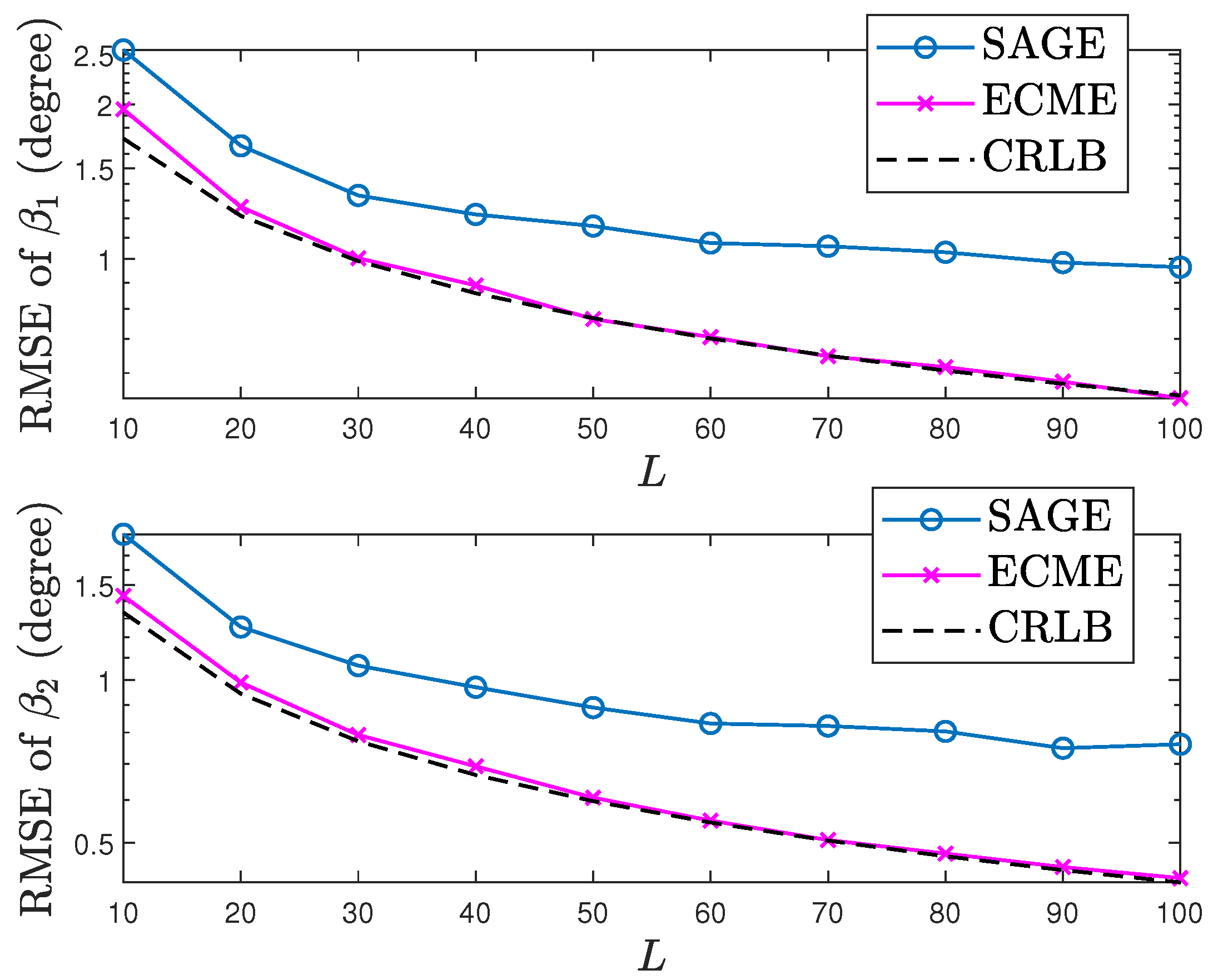
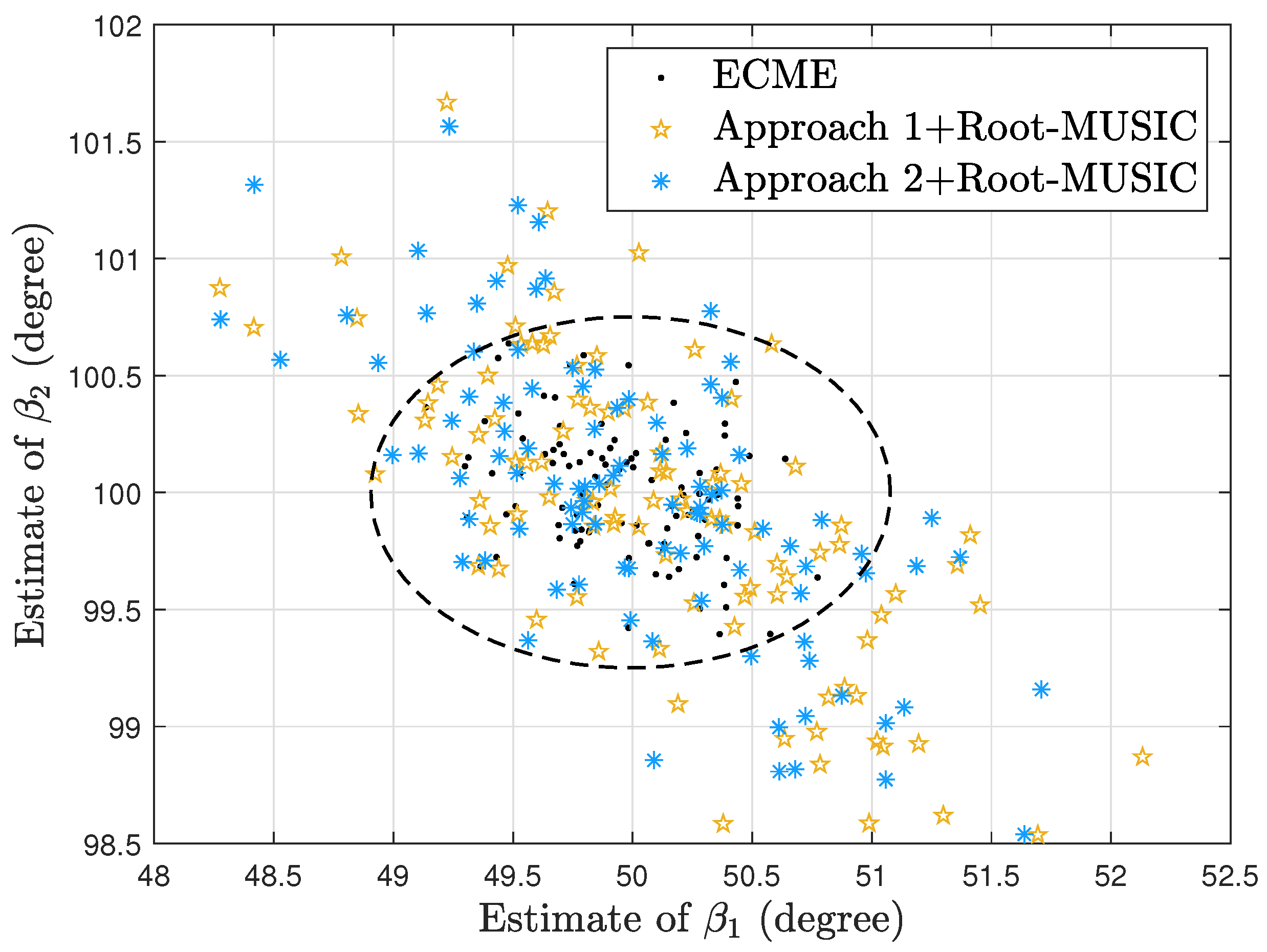
4. Simulation Results

Simulation results are provided to confirm the effectiveness of the ECME algorithm, i.e., the ECME algorithm is able to obtain the ML estimate of β in (3). We set V = 2 , β 1 = 50 , W = 6 , β 2 = 100 , and δ = [ 1 2 3 4 2 10 ] T . Algorithm 1 is used to obtain β ( d ) in (20) and β ( u + 1 ) β ( u ) 2 0 . 001 is adopted as the stopping criterion. The ECME algorithm is given an accurate initial point for obtaining the ML estimate of β . In Figure 1 and Figure 2, we consider the coherent (or fully correlated) source model with [25]
O = γ γ γ γ = γ 0 0 γ 1 1 1 1 γ 0 0 γ .
In Figure 3, we consider the partly correlate source model with
O = 5 4 4 5 = 5 0 0 5 1 4 / 5 4 / 5 1 5 0 0 5 .
In Figure 1 and Figure 2, we compare the root mean square error (RMSE) performance of the ECME algorithm with the CRLB [4,5]. In addition, we simulate the second space-alternating generalized EM (SAGE) algorithm for uncorrelated sources in [20], and this SAGE algorithm adopts the same simulation settings in [20]. Each RMSE is based on 2000 independent trials and the two algorithms share the same initial point. As expected, the ECME algorithm obtains smaller RMSEs than the SAGE algorithm. More importantly, the ECME algorithm attains the CRLB of β when the number of snapshots L or γ is large, which coincides with the well-known conclusion that the stochastic CRLB of β can be achieved asymptotically by the stochastic ML estimator of β [2]. Hence, the ECME algorithm is able to obtain the stochastic ML estimate of β in (3) given an accurate initial point.
In Figure 3, we compare the ECME algorithm with two subspace-based algorithms, which utilize the state-of-the-art subspace separation approaches in [17,18] and are called “Approach 1+Root-MUSIC” and “Approach 2+Root-MUSIC”, respectively. The three algorithms process the same snapshots of each trial. As expected, the ECME algorithm yields more closely spaced estimates of ( β 1 , β 2 ) centered on ( 50 , 100 ) since in DOA estimation, the ML technique offers the highest advantage in terms of accuracy.

5. Conclusions

In this paper, we employed and designed the ECME algorithm for stochastic ML direction finding, where sources may be correlated, in unknown nonuniform noise. Theoretical analysis indicated that the ECME algorithm is computationally efficient and operationally stable. Simulation results confirmed that the ECME algorithm can efficiently obtain the ML based DOA estimate of each stochastic source.

Author Contributions

This paper was co-authored by M.-Y.G. and B.L. Conceptualization, M.-Y.G.; methodology, M.-Y.G.; software, M.-Y.G.; validation, M.-Y.G. and B.L.; formal analysis, M.-Y.G.; investigation, M.-Y.G.; resources, B.L.; data curation, M.-Y.G.; writing—original draft preparation, M.-Y.G.; writing—review and editing, B.L.; supervision, B.L.; funding acquisition, B.L. All authors have read and agreed to the published version of the manuscript.

Funding

This research was funded by the Open Research Project of Jiangsu Provincial Key Laboratory of Photonic and Electronic Materials Sciences and Technology, grant number NJUZDS 2022-008.

Institutional Review Board Statement

Not applicable.

Informed Consent Statement

Not applicable.

Data Availability Statement

The data presented in this study are available on request from the corresponding author. The data are not publicly available, due to the data in this paper not being from publicly available datasets but obtained from the simulation of the signal models listed in the paper.

Conflicts of Interest

The authors declare no conflict of interest.

References

  1. Stoica, P.; Nehorai, A. MUSIC, maximum likelihood, and Cramer-Rao bound. IEEE Trans. Acoust. Speech Signal Process. 1989, 37, 720–741. [Google Scholar] [CrossRef]
  2. Stoica, P.; Nehorai, A. Performance study of conditional and unconditional direction-of-arrival estimation. IEEE Trans. Acoust. Speech Signal Process. 1990, 38, 1783–1795. [Google Scholar] [CrossRef]
  3. Stoica, P.; Larsson, E.G.; Gershman, A.B. The stochastic CRB for array processing: A textbook derivation. IEEE Signal Process. Lett. 2001, 8, 148–150. [Google Scholar] [CrossRef]
  4. Pesavento, M.; Gershman, A.B. Maximum-likelihood direction-of-arrival estimation in the presence of unknown nonuniform noise. IEEE Trans. Signal Process. 2001, 37, 1310–1324. [Google Scholar] [CrossRef]
  5. Gershman, A.B.; Pesavento, M.; Stoica, P.; Larsson, E.G. The stochastic CRB for array processing in unknown noise fields. In Proceedings of the 2001 IEEE International Conference on Acoustics, Speech, and Signal Processing, Proceedings (Cat. No. 01CH37221), Salt Lake City, UT, USA, 22–27 May 2001. [Google Scholar]
  6. Delmas, J.; Abeida, H. Stochastic Cramer-Rao bound for noncircular signals with application to DOA estimation. IEEE Trans. Signal Process. 2004, 52, 3192–3199. [Google Scholar] [CrossRef]
  7. Abeida, H.; Delmas, J. Gaussian Cramer-Rao bound for direction estimation of noncircular signals in unknown noise fields. IEEE Trans. Signal Process. 2005, 53, 4610–4618. [Google Scholar] [CrossRef]
  8. Ziskind, I.; Wax, M. Maximum likelihood localization of multiple sources by alternating projection. IEEE Trans. Acoust. Speech Signal Process. 1988, 36, 1553–1560. [Google Scholar] [CrossRef]
  9. Miller, M.I.; Fuhrmann, D.R. Maximum-likelihood narrow-band direction finding and the EM algorithm. IEEE Trans. Acoust. Speech Signal Process. 1990, 38, 1560–1577. [Google Scholar] [CrossRef]
  10. Chung, P.; Bohme, J.F. Comparative convergence analysis of EM and SAGE algorithms in DOA estimation. IEEE Trans. Signal Process. 2001, 49, 2940–2949. [Google Scholar] [CrossRef]
  11. Gong, M.; Lyu, B. Alternating maximization and the EM algorithm in maximum-likelihood direction finding. IEEE Trans. Veh. Technol. 2021, 70, 9634–9645. [Google Scholar] [CrossRef]
  12. EM and SAGE Algorithms for DOA Estimation in the Presence of Unknown Uniform Noise. Available online: https://arxiv.org/abs/2208.07510 (accessed on 16 August 2022).
  13. Zoubir, A.M.; Aouada, S. High resolution estimation of directions of arrival in nonuniform noise. In Proceedings of the 2004 IEEE International Conference on Acoustics, Speech, and Signal Processing, Montreal, QC, Canada, 17–21 May 2004. [Google Scholar]
  14. Madurasinghe, D. A new DOA estimator in nonuniform noise. IEEE Signal Process. Lett. 2005, 12, 337–339. [Google Scholar] [CrossRef]
  15. Liao, B.; Chan, S.; Huang, L.; Guo, C. Iterative methods for subspace and DOA estimation in nonuniform noise. IEEE Trans. Signal Process. 2016, 64, 3008–3020. [Google Scholar] [CrossRef]
  16. Liao, B.; Huang, L.; Guo, C.; So, H.C. New approaches to direction-of-arrival estimation with sensor arrays in unknown nonuniform noise. IEEE Sens. J. 2016, 16, 8982–8989. [Google Scholar] [CrossRef]
  17. Esfandiari, M.; Vorobyov, S.A.; Alibani, S.; Karimi, M. Non-iterative subspace-based DOA estimation in the presence of nonuniform noise. IEEE Signal Process. Lett. 2019, 26, 848–852. [Google Scholar] [CrossRef]
  18. Esfandiari, M.; Vorobyov, S.A. A novel angular estimation method in the presence of nonuniform noise. In Proceedings of the ICASSP 2022—2022 IEEE International Conference on Acoustics, Speech and Signal Processing (ICASSP), Singapore, 23–27 May 2022. [Google Scholar]
  19. Chen, C.E.; Lorenzelli, F.; Hudson, R.E.; Yao, K. Stochastic maximum-likelihood DOA estimation in the presence of unknown nonuniform noise. IEEE Trans. Signal Process. 2008, 56, 3038–3044. [Google Scholar] [CrossRef]
  20. EM-Type Algorithms for DOA Estimation in Unknown Nonuniform Noise. Available online: https://arxiv.org/abs/2211.02458 (accessed on 4 November 2022).
  21. Liu, C.; Rubin, D.B. The ECME algorithm: A simple extension of EM and ECM with faster monotone convergence. Biometrika 1994, 81, 633–648. [Google Scholar] [CrossRef]
  22. Jaffer, A.G. Maximum likelihood direction finding of stochastic sources: A separable solution. In Proceedings of the ICASSP-88, International Conference on Acoustics, Speech, and Signal Processing, New York, NY, USA, 11–14 April 1988. [Google Scholar]
  23. Stoica, P.; Nehorai, A. On the concentrated stochastic likelihood function in array signal processing. Circuits Syst. Signal Process. 1995, 14, 669–674. [Google Scholar] [CrossRef]
  24. Bresler, Y. Maximum likelihood estimation of linearly stmctured covariance with application to antenna array processing. In Proceedings of the 4th ASSP Workshop Spectrum Estimation Modeling, Minneapolis, MN, USA, 3–5 August 1988. [Google Scholar]
  25. Stoica, P.; Ottersten, B.; Viberg, M.; Moses, R.L. Maximum likelihood array processing for stochastic coherent sources. IEEE Trans. Signal Process. 1996, 44, 96–105. [Google Scholar] [CrossRef]
  26. Dempster, A.P.; Laird, N.M.; Rubin, D.B. Maximum likelihood from incomplete data via the EM algorithm. J. Roy. Statist. Soc. Ser. B (Methodol.) 1977, 39, 1–38. [Google Scholar]
  27. Rhodes, I.B. A tutorial introduction to estimation and filtering. IEEE Trans. Autom. Control 1971, 16, 688–706. [Google Scholar] [CrossRef]
  28. Jeff Wu, C.F. On the convergence properties of the EM algorithm. Ann. Statist. 1983, 11, 95–103. [Google Scholar]
  29. Stoica, P.; Gershman, A.B. Maximum-likelihood DOA estimation by data-supported grid search. IEEE Signal Process. Lett. 1999, 6, 273–275. [Google Scholar] [CrossRef]
  30. Malioutov, D.; Cetin, M.; Willsky, A.S. A sparse signal reconstruction perspective for source localization with sensor arrays. IEEE Trans. Signal Process. 2005, 53, 3010–3022. [Google Scholar] [CrossRef]
Figure 1. Relationship between the RMSE performance of the ECME algorithm and the CRLB. γ = 2 , β 1 ( 0 ) = 45 , O ( 0 ) = I V , β 2 ( 0 ) = 95 , and Q ( 0 ) = I W .
Electronics 12 02191 g001
Figure 2. Relationship between the RMSE performance of the ECME algorithm and the CRLB. L = 100 , β 1 ( 0 ) = 45 , O ( 0 ) = I V , β 2 ( 0 ) = 95 , and Q ( 0 ) = I W .
Electronics 12 02191 g002
Figure 3. Estimates of ( β 1 , β 2 ) obtained from the ECME and two subspace-based algorithms under 100 independent trials. β 1 ( 0 ) = 45 , β 2 ( 0 ) = 95 , O ( 0 ) = I V , L = 100 , and Q ( 0 ) = I W .
Electronics 12 02191 g003
Disclaimer/Publisher’s Note: The statements, opinions and data contained in all publications are solely those of the individual author(s) and contributor(s) and not of MDPI and/or the editor(s). MDPI and/or the editor(s) disclaim responsibility for any injury to people or property resulting from any ideas, methods, instructions or products referred to in the content.

