Article

Deep Cascade AdaBoost with Unsupervised Clustering in Autonomous Vehicles

1
State Key Laboratory of CEMEE, Luoyang 471000, China
2
School of Telecommunications Engineering, Xidian University, Xi’an 710071, China
3
Science and Technology on Complex System Control and Intelligent Agent Cooperation Laboratory, Beijing Electro-Mechanical Engineering Institute, Beijing 100000, China
*
Author to whom correspondence should be addressed.
Electronics 2023, 12(1), 44; https://doi.org/10.3390/electronics12010044
Submission received: 1 November 2022 / Revised: 6 December 2022 / Accepted: 10 December 2022 / Published: 22 December 2022
(This article belongs to the Special Issue Advances and Applications of Networking and Multimedia Technologies)

Abstract

:
In recent years, deep learning has achieved excellent performance in a growing number of application fields. With the help of high computation and large-scale datasets, deep learning models with huge parameters constantly enhance the performance of traditional algorithms. Additionally, the AdaBoost algorithm, as one of the traditional machine learning algorithms, has a minimal model and performs well on small datasets. However, it is still challenging to select the optimal classification feature template from a large pool of features in any scene quickly and efficiently. Especially in the field of autonomous vehicles, images taken by onboard cameras contain all kinds of targets on the road, which means the images are full of multiple features. In this paper, we propose a novel Deep Cascade AdaBoost model, which effectively combines the unsupervised clustering algorithm based on deep learning and the traditional AdaBoost algorithm. First, we use the unsupervised clustering algorithm to classify the sample data automatically. We can obtain classification subsets with small intra-class and large inter-class errors by specifying positive and negative samples. Next, we design a training framework for Cascade-AdaBoost based on clustering and mathematically demonstrate that our framework has better detection performance than the traditional Cascade-AdaBoost framework. Finally, experiments on the KITTI dataset demonstrate that our model performs better than the traditional Cascade-AdaBoost algorithm in terms of accuracy and time. The detection time was shortened by 30 % , and the false detection rate was reduced by 20 % . Meanwhile, the training time of our model is significantly shorter than the traditional Cascade-AdaBoost algorithm.

1. Introduction

Deep learning models have demonstrated superior performance in computer vision, speech recognition, and natural language processing (NLP) over the past few years. Most of these models achieve state-of-the-art performance. The significant progress in deep learning relies mainly on the following two aspects. On one hand, the convolutional neural network (CNN) is used to extract high-dimensional visual features from images, which can effectively mine latent semantic information hidden in data. The deep learning model has been widely used in object detection and tracking [1,2,3,4,5,6,7]. On the other hand, deep learning typically uses deeper and larger models with numerous parameters to achieve higher precision and accuracy.
Before the explosion of deep learning, traditional machine learning algorithms dominated. Traditional machine learning algorithms have achieved great success in various aspects such as image classification [8,9], human action recognition [10,11], and face detection [12,13]. They have been the primary choice even in most current applications in the industry for the following reasons. First, traditional machine learning algorithms utilize handcrafted features rich in expert experience and require only a small number of samples to achieve the desired results. In addition, lightweight models and slight computational complexity make it possible to quickly deploy in arbitrarily complex scenarios without high hardware costs. However, as the size of data increases, the performance of traditional machine learning algorithms will gradually fall into a bottleneck. It takes work to see a significant performance improvement. Furthermore, traditional algorithms rely heavily on manually designed features. Some excellent features, such as HAAR [14,15], HOG [16,17] and LBP [12,18], have been practiced in practical applications with good results. Nevertheless, there is no good solution to finding the best features in a large-scale feature base. The features required for different tasks also vary, making it difficult to expand our algorithm.
In [19], they used the algorithm for feature extraction based on transfer learning, feature selection and optimization of the parameters of a multi-layer neural network based on meta-heuristic optimization, so as to improve the accuracy of the classification of monkeypox images. This is the up-to-date application of feature extraction in the medical field. In the field of autonomous vehicles [20,21], how to quickly and accurately realize the vehicle detection of the pictures taken by onboard cameras is extremely important. In the same way, it is not easy because the pictures taken by the onboard camera contain a massive amount of information. In addition to the vehicles we need to detect, the pictures also include a lot of redundant information, such as lane lines, pedestrians, street trees, road signs, traffic lights, buildings and other targets. How to extract vehicle features from so many targets is extremely difficult. Moreover, the vehicle is constantly moving, that is to say, the target and scene in the picture are changing, which undoubtedly further increases the difficulty of vehicle detection.
This is the main problem to be solved in this work. To handle it, we proposed an algorithm called Deep Cascade AdaBoost, which combines the advantages of the AdaBoost algorithm and deep unsupervised clustering.
Similar to the traditional AdaBoost-based detection task, we also use the structure of Cascade-AdaBoost to construct a classifier with a higher detection rate by concatenating several strong classifiers. To efficiently select the best features of vehicles from the feature pool, we designed a classification-based Cascade-AdaBoost. In our approach, we combine clustering with deep learning. Through this method, we will obtain a feature extractor and then initialize the feature extractor of the network of the data waiting to be solved, which contains little or no data labels. This is the core of the method we proposed. The whole framework is shown in detail in Figure 1. The whole process consists of clustering the features and then updating the parameters of the network based on the results of clustering, which are considered as pseudo-labels so that the network can predict these pseudo-labels. The two processes are carried out in turn. Though this process seems quite simple, it can perform better than previous unsupervised approaches.
Similar to supervised learning, unsupervised learning also has a division between positive and negative samples. In our work, we choose the samples dominated by vehicles as the positive samples. On the contrary, those oriented to the background such as sky, trees and buildings can be classified as negative samples. The traditional AdaBoost algorithm filters the negative samples recognized as a whole randomly. Then, it increases the weights of the negative samples that are difficult to separate for multiple feature extraction for classification. In the case of the cascade classifier, it does not take into account the influence of the overall distribution of negative samples on the performance of the classifier nor the ease of separating negative samples on the performance of the classifier, taking a long time to separate the images. The negative samples are categorized into primary and secondary levels, and the central part is selected with priority, which can greatly reduce the training time. Then, at the same time, the sorting of classification tasks combined with scene analysis can also significantly reduce the detection time.
In our work, firstly, we classify all negative samples. The classification algorithm implements the classification of negative samples by filtering the original randomly large number of negative samples into several classes with fewer differences. Then, a hierarchical training approach uses only one class of negative samples per layer. In each layer of training, the best artificial features based on that class of negative samples are found by traversing the feature library. Finally, we concatenate the classifiers of all layers in turn to form the final strong classifier. Reducing the intra-class interval by sample classification not only reduces the computational effort of traversing the feature pool, but also helps us to find the best features. By concatenating all classifiers in series, we can ensure that we have found the best features that distinguish positive samples from all negative samples.
We also strain every nerve to perform unsupervised clustering on the data of an unknown scene. We combine unsupervised clustering with the previously introduced hierarchical Cascade AdaBoost algorithm to make it possible to efficiently detect vehicles in arbitrary scenes. In addition, we note that the current state-of-the-art deep unsupervised clustering algorithm that uses CNN to extract image features achieves end-to-end clustering and the best performance on data with an unbalanced distribution. In our work, we incorporate this approach, allowing us to achieve clustering of samples with unbalanced distribution in random scenes.
We designed the corresponding experiment to verify the superiority of our model. We chose the KITTI dataset as our training and test dataset. As one of the important datasets in autonomous driving scenarios, the KITTI dataset includes most of the scenes in our daily life and the images in it are ample enough to support our work. The performance on the test dataset demonstrates that our model takes less time while improving detection accuracy. Specifically, the detection time accomplished by our model in a shorter training time was shortened by 30 % , and the false detection rate was reduced by 20 % in our test dataset.
In summary, the main contributions of this work are as follows:
  • We creatively propose a framework that combines deep learning with traditional machine learning. As we describe throughout this article, our model can implement arbitrary scene object detection tasks, greatly enriching the application of traditional detection algorithms. By establishing the relationship between clustering and the AdaBoost algorithm, we obtain the Deep Cascade AdaBoost model.
  • We design a training method based on Cascade-AdaBoost with multi-category samples. Instead of global samples, ordered categorical samples are used, and then the hierarchical training models are cascaded. In this paper, we also demonstrate the effectiveness of our method with a theoretical formulation.
  • We compare with the traditional AdaBoost model on multiple classes of vision tasks, and the model we proposed achieves the best results in both accuracy and time. In our test dataset, the detection time was shortened by 30 % , and the false detection rate was reduced by 20 % , even though our model was accomplished in a shorter training time. In addition, we add the additional interference to the experiment and find that the new model has a remarkable ability to screen out external noise.

2. Materials and Methods

In this section, we briefly introduce some recent developments in two topics, Deep clustering and traditional learning method, which are closely related to our work.

2.1. Deep Clustering

As a traditional method of unsupervised learning, the purpose of clustering is to classify similar data into a cluster based on specific similarity standards. The weakness of the traditional algorithm of clustering is apparent. It is inefficient and performs poorly in high-dimensional data and high computational complexity in large-scale datasets. Along with density estimation, clustering is a family of standard unsupervised learning methods. With the development of deep learning, deep neural networks (DNNs) can be used to transform the data into more clustering-friendly representations because of their inherent characteristics of highly non-linear transformation [22]. Deep embedding clustering (DEC) [23,24] uses auto-encoders as the network architecture, minimizing the KL divergence between the distribution of the soft label and the distribution of the auxiliary target to improve the quality of clustering. JULE [25] uses the hierarchical clustering method and extracts image features using CNN. Deep adaptive image clustering (DAC) is a method of image clustering based on single-stage convolutional networks [26]. Our paper builds upon the work of Caron et al., in which k-means is used to cluster the visual representations.

2.2. Traditional Learning Method

Machine learning is the science of artificial intelligence (AI), which uses data and past experience to improve algorithms and achieve realistic simulations of how humans learn. After decades of development, machine learning has become a very mature theory and system, showing a powerful vitality in solving complex problems in engineering applications and scientific fields. For example, decision tree is a typical machine learning algorithm [27,28,29,30]. By selecting an optimal feature recursively, the training data set is segmented according to the optimal feature to classify data efficiently. Using multiple tree classifiers to classify and predict data, random forest is one of the essential methods of machine learning [31,32]. The EM algorithm considers the probabilistic model with hidden variables to achieve maximum likelihood estimation of the observed data [33,34]. Boosting only needs rough basic algorithms and can achieve a high-precision prediction model through repeated adjustments [35,36]. As the most representative of the Boosting algorithm, AdaBoost achieves great success. The cascade classifier is a qualitative leap to detect the AdaBoost algorithm. It connects several classifiers with good classification performance in series to detect objects faster and more accurately. However, traditional machine learning algorithms have encountered difficulties in the face of large datasets The processing of multiple parameters also remains a complex problem for machine learning.

2.3. Dataset for AdaBoost Training

The choice of training dataset affects the performance of the final trained detectors, so we used the KITTI dataset, one of the most important datasets for evaluating computer vision algorithms in autonomous driving scenarios, as the training dataset. KITTI is diverse and contains images taken in urban, rural and highway scenes with up to 15 vehicles and 30 pedestrians, as well as varying degrees of occlusion and truncation. The negative background contains sky, trees, buildings, roads, traffic signs, etc., which is closely related to the presence of vehicles and helps to discriminate between vehicles and non-vehicles when running the detector in real video. In addition, KITTI includes images of vehicles at different times of the day under different lighting conditions, which helps the final vehicle detector to adapt to different environments. We only consider the vehicle detection task in the road context. So we divide the training dataset and the test dataset in a 2:1 ratio in our work.

2.4. Data Processing

The training of AdaBoost requires positive and negative samples Thus we need to segment the original image. The KITTI dataset provides training labels for cropping out vehicles from each image in the training set to extract frontal samples. We prioritized images with unobstructed vehicles and precise bodywork. Then we extracted frontal samples containing both the front and back of the vehicles. The vehicle samples contain vehicles with different orientations and brightness, which match the images taken in real scenes. After cropping the vehicles, we extracted negative samples from the remaining area to ensure that the negative samples only contained objects other than vehicles in the background. In addition to these negative samples from KITTI, we also select real-world relevant databases containing images of roads, trees, skies, buildings, etc. as negative samples for training. During the training process of AdaBoost, the ability of the classifiers to classify negative samples increases as the STAGE increases, leading to difficulties in generating negative samples. Therefore, it is necessary to provide as many negative samples as possible to support the training. We set the ratio of positive and negative samples to 1:5 during training to ensure the classifier has better learning ability.

3. Proposed Methodology

3.1. Deep Cascade AdaBoost

In this section, we elaborate on the deep unsupervised clustering and classifier based on cascade AdaBoost. We also mathematically prove that our model performs better than the traditional Cascade-AdaBoost algorithm in terms of accuracy and time.

3.1.1. Deep Unsupervised Clustering

Convolution networks can map images to fixed dimensionality spaces and provide good visual features for image clustering. In this work, we use the f θ to represent the feature mapping function, where θ is the corresponding parameter vector. We expect to find a parameter θ in the prescient image train set X = x 1 , x 2 , , x n , which can make f θ perform well in the forecast task.
In traditional classification prediction methods, the values of these parameters are given by supervised learning. Briefly, for each image x, there is a label to indicate that it belongs to a specific predefined category. Contrary to previous work, we take the vectors obtained in the penultimate layer of ConvNet as a feature, then cluster the output of ConvNet and optimize it by using the subsequent cluster assignment as a “pseudo-label”. We define a potential pseudo label z n and the corresponding linear classifier V for each image n. Pseudo tags can be updated by minimizing exponential loss functions. These cluster-based methods alternate between learning parameters θ and V and update pseudo-label z n . By optimizing the function:
θ , V m i n = 1 N n = 1 N ( y n , V f θ ( x n ) ) .
where is the loss function, also known as the negative log-softmax function. The small-batch stochastic gradient descent method is used to optimize the loss function. During the optimization process, label z n can be redistributed.
Clustering technology has developed rapidly in recent years, and various clustering methods are put forward and improved constantly. Even different clustering methods are proposed for different data. In our work, we will focus on Caron and other Deep Cluster frameworks through the k-means to activate potential clustering targets. The pre-experiment results show that the choice of different clustering algorithms has no evident influence on the results, so we choose the standard k-means method. With the characteristic which is produced by the convolution network f θ ( x n ) as input, we gather them into k different groups by solving the following optimization problem:
C R d × k m i n n = 1 N y n 0 , 1 k s . t . y n 1 = 1 m i n C y n f θ ( x n ) 2 2
here, C is the learned centroid matrix, where each column corresponds to a centroid, k is the number of centroids, z n is a binary vector with only one non-zero term, and the best clustering assignment is learned for each image n. These assignments are used as pseudo labels to update the parameters in Equation (1).
However, in this approach, it is inevitable to encounter two problems. One of the problems is that of empty clusters due to the lack of constraint of empty clusters. In order to solve this problem, we can place restrictions on the minimum number of samples per cluster. Nevertheless, it requires calculating the entire dataset, which costs too much. So when a certain cluster is empty, we randomly select a non-empty cluster and add some small perturbations to make it a new centroid of the empty cluster. Meanwhile, the samples belonging to the non-empty cluster also belong to the new cluster. The other problem is trivial parametrization. A large amount of data is clustered into a small number of classes. There exists one extreme situation where all the data is clustered into one class. Under the circumstances, the network may produce the same output no matter what the input is. The solution to this problem is to sample the samples according to classes or pseudo-labels evenly.

3.1.2. Classifier-Based Cascade AdaBoost

AdaBoost algorithm is a kind of Boosting algorithm which can modify weak learning classifiers to strong learning classifiers. This kind of algorithm usually trains the base classifiers from the initialized sample first, and the performance of these classifiers is better than that of random guessing. We can adjust the distribution of the weight of the samples through the performance of the base classifier in the initial sample, so that the samples distributed into error categories in the previous classification will receive more attention in the following training stage. Then, the next base classifier is trained with the adjusted sample. After iterating the specified number of times, all the base classifiers are weighted to form the final classifier. The following is a detailed description of the AdaBoost algorithm.
By minimizing the exponential loss function, the AdaBoost algorithm can make s i g n ( H ( x ) ) reach the Bayesian optimal error rate. Through that, the classification error rate is the minimum. Moreover, the exponential loss function is continuously differentiable and is used as the optimization target.
In the AdaBoost algorithm, h 1 is a weak classifier generated by acting on the initialized distribution of weight through a direct basis learning algorithm. Then through one iteration, the weight updates. Based on the previous iteration of the sample, weight distribution of D t , h t is obtained by the base learning algorithm. The weight of the classifier should be made to minimize the exponential function.
For the weak classification h t ( x ) , the exponential function is:
e x p ( α t h t ( x ) | D t ) = E x D t [ e α t f ( x ) h t ( x ) ] E x D t [ e α t Π ( f ( x ) = h t ( x ) ) + [ e α t Π ( f ( x ) h t ( x ) ) ] = e α t P x D t ( f ( x ) = h t ( x ) ) + e α t P x D t ( f ( x ) h t ( x ) ) = e α t ( 1 ϵ t ) + e α t ϵ t
here, ϵ t = P x D t ( f ( x ) h t ( x ) ) . Consider the derivative of the loss function:
e x p ( α t h t ( x ) | D t ) α t = e α t ( 1 ϵ t ) + e α t ϵ t
We can solve for this when Equation (5) is equal to 0:
α t = 1 2 ln 1 e t e t
Plug Equation (6) into Equation (5), we have:
e x p ( α t h t ( x ) | D t ) = ( 1 ϵ t ) ( ϵ t )

3.1.3. Cascade AdaBoost

The Adaboost algorithm can train a strong classifier, but only one strong classifier cannot guarantee the detection accuracy. Accordingly, the combination of several strong classifiers is needed to generate a classifier with a high correct rate. A cascade of face classifiers is a decision tree where a classifier is trained and formed at each stage to detect almost all frontal faces while rejecting a certain fraction of non-face patterns. Those image-windows that are not rejected by a stage classifier in the cascade sequence will be processed by the continuous stage classifiers. The cascade architecture can dramatically increase the speed of the detector by focusing attention on promising regions of the images.
For h t , we have
e x p ( α t h t ( x ) | D t ) = E x D t [ e α t f ( x ) h t ( x ) ] = e α t ( 1 ϵ t ) + e α t ϵ t = ( 1 ϵ t ) ( ϵ t )
For every t, ϵ t < ϵ t , ( 1 ϵ t ) ( ϵ t ) < ( 1 ϵ t ) ( ϵ t ) , so we have e x p ( α t h t ( x ) | D t ) < e x p ( α t h t ( x ) | D t ) .
e x p ( H ( x ) | D ) = E x D [ e f ( x ) H ( x ) ] = E x D [ e f ( x ) t = 1 T α t h t ( x ) ] = t = 1 T ( 1 ϵ t ) ( ϵ t )
For every t, ϵ t < ϵ t , so we have e x p ( H ( x ) | D t ) < e x p ( H ( x ) | D t ) .
The steps of the algorithm of our method are shown below in Algorithm 1.
Algorithm 1:The Deep Cascade AdaBoost
Input: Initialize the following parameters.
(1) Feature extraction function: f θ ;
(2) The parameter vector: θ ;
(3) Linear classifier W;
(4) the number of classifications k;
Output: the results of Clustering:
The center of mass matrix C and k cluster samples N k
for n = 1 ; n k ; n + + do
Initialize the weights w i = 1 N k , i = 1 , 2 , , N k
   for  t = 1 ; t M ; j + +  do
      (a) Fit a classifier G t ( x ) to the training set
      (b) Compute e t = i = 1 N k w i I ( y i G t ( x i ) ) i = 1 N k w i
      (c) Compute α t = ln ( 1 e t e t )
      (d) Set w i w i · e x p ( α t · I ( y i G t ( x i ) ) )
      (e) Set f i ( X ) = t = 1 N k α t G t ( x )
      Output f ( n ) ( X ) = s i g n ( f M ( X ) )
   endfor
Output: f ( X ) = n = 1 k f ( n ) ( X )
endfor

3.1.4. Clustering-Based Cascade AdaBoost

Compared with the performance of the original algorithm, our method improves a lot owing to achieving optimization index loss function. Under the same number of iteration layers, the algorithm we proposed has better classification performance. In order to achieve the specified performance effect, we train fewer layers than the original algorithm. It means that, compared with the original algorithm, we only need a few features to accurately distinguish the positive samples from the negative ones.
G k ( H k ( x ) | T k ) > G k ( H ( x ) | T )
Here, k represents the class k samples after classification, and the number of training layers is T k ; G k represents the classification effect of class k things; T represents the number of training layers of unclassified samples, T k < < T , and k = 1 n < = T .
k = 1 n t = 1 T k ( 1 ϵ t ) ( ϵ t ) < t = 1 T ( 1 ϵ t ) ( ϵ t )
In actual training, it is easy to find T i and T that satisfy the above relation. In fact, only three to five layers for each category can satisfy the relation. Moreover, the total sample of regular training needs a large number of layers; so, under most conditions, k = 1 n < T .

3.2. Experiment

In this section, we conduct experiments to validate the effectiveness of the Deep Cascade AdaBoost we proposed. To evaluate our proposed method, we apply it to a vehicle detection system on the road. This system contains two modules, the first module is the clustering algorithm to cluster the ROI, which is the first focus of this paper. The second module is the second focus of this paper, where we train the clustered data for hierarchical cascade enhancement.

3.2.1. Clustering

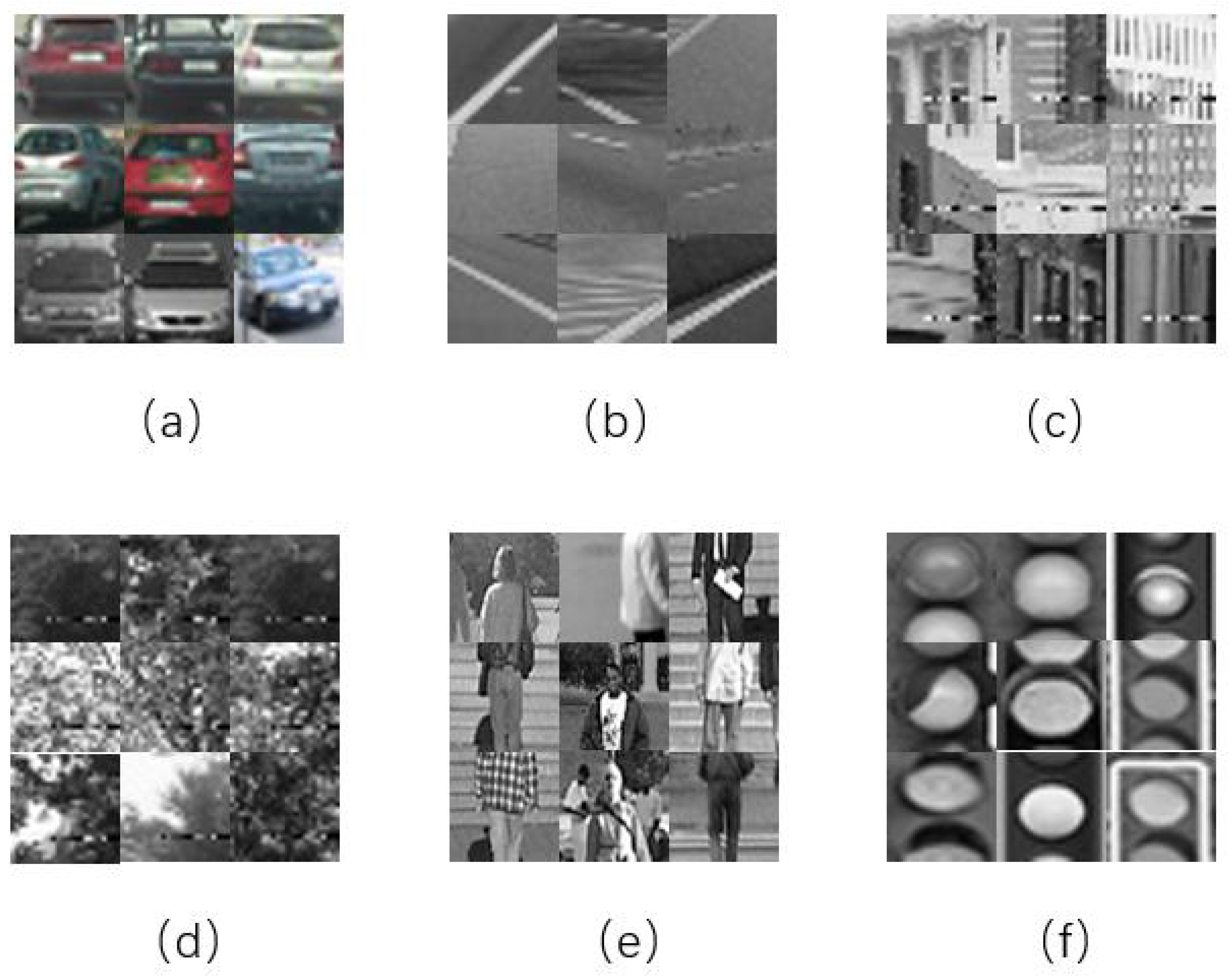
The experiments are all carried out on a workstation with NVIDIA GeForce RTX 2060. Our implementation of deep clustering is based on the framework described in DeepCluster [37]. In this work, all input images are simply resized to the size of 227 × 227 before clustering to ensure the utilization of the standard AlexNet architecture. We follow the method in the previous section to obtain positive and negative samples. For all samples, we use the state-of-the-art unsupervised clustering method for clustering. We set the number of species of clusters to 6 and obtained a more satisfactory result of clustering. The vehicle samples were correctly clustered in the final clustering results with 98 % accuracy. In the meantime, the model also clustered roads, buildings, skies and plants accurately, which is consistent with what we observed in practice. Below are the examples of a figure caption in Figure 2.

3.2.2. Multi-Cascade-AdaBoost

The multi-layer cascade classifier is a series of individual cascade classifiers. Each cascade classifier is composed of individual stages with a strong classifier consisting of weak classifiers combined with the AdaBoost algorithm. The cascade structure ensures that the final classifier has the ability to classify positive and negative samples with high accuracy. In order to compare the performance of our method with traditional methods, we train with three features, HAAR, LBP and HOG. Then, we compare the detection results.
In order to optimize the training process, we adjust some of the more critical training parameters.
  • Number of stages. Usually, increasing the number of stages results in a more accurate detector, but it needs more time to train the model. Higher stages may also require more training images, and the demand for such images tends to grow exponentially, while the improvement for detectors is minimal. In our training, the number of stages was set to 30.
  • Object training size. By default, the training function sets the size of the samples in the instance to [24 24]. To make the training results more accurate, we refer to the expected size of the target in the actual image. Finally, the training sample size is set to [30 30].
  • False alarm rate. Higher values of alarm rate tend to require more cascading stages to achieve reasonable detection accuracy and increase the memory consumption of the model. Lower values increase the model complexity. The alarm rate generally defaults to 0.5, and we set the alarm rate to 0.3 in order to use a smaller number of stages.
  • Feature Selection. Using AdaBoost in the evaluation method of vehicle detection, the classical three features are HAAR features, LBP features and HOG features. HAAR shows the information of light and dark transformation of image pixel values. LBP describes the texture information corresponding to the local extent of the image and HOG reacts to the edge gradient information of the image. In this work, we use these three features above to learn the vehicle detector and observe the performance of vehicle detection with different features.

4. Results and Discussion

This section shows the performance of our algorithm from the training process to the test results compared to the traditional algorithm.

4.1. Effect on the Training Process

In Table 1, we recorded the time of training the classifier, the number of stages to terminate the training, and the number of features found for several methods.
By comparing the results shown in Table 1, it can be observed that the AdaBoost algorithm using HAAR features takes the longest time to train the model, utilizing the largest number of features and stages of model convergence. Using LBP has the smallest value among all of them. In addition, we can notice that the AdaBoost algorithm combining HAAR, LBP and HOG features has a significant decrease in training time, the number of features and the number of stages compared to the original algorithm after using the framework of clustering-cascading-AdaBoost. This indicates that our method helps to find the best features, making the model reach convergence as early as possible.

4.2. Comparison of Detector Performance

To evaluate the performance of these methods, we recorded the True Positive Rate ( T P R ) and the False Positive Rate ( F P R ). TPR indicates the percentage of correctly identified vehicle samples. It was calculated using Equation (11)
T P R = T P T P + F N
where T P is the number of true positive samples and F N is the number of false negative samples.
The false positive rate indicates the probability that a positive vehicle sample is predicted to be a negative sample. It was calculated using Equation (12)
F P R = F P F P + T N
where F P is the number of false positive samples and T N is the number of true negative samples.
Table 2 summarizes the results obtained for the six vehicle detection methods on the test dataset. According to the results in Table 2, the HAAR feature combined with the AdaBoost method has the best detection rate and false detection rate in vehicles, followed by the HOG feature, and the LBP feature is the least. Meanwhile, Table 2 also displays that the detection rate and false detection rate of all three features combined with the AdaBoost algorithm are greatly improved after the clustering algorithm, which shows the superiority of the method we proposed.
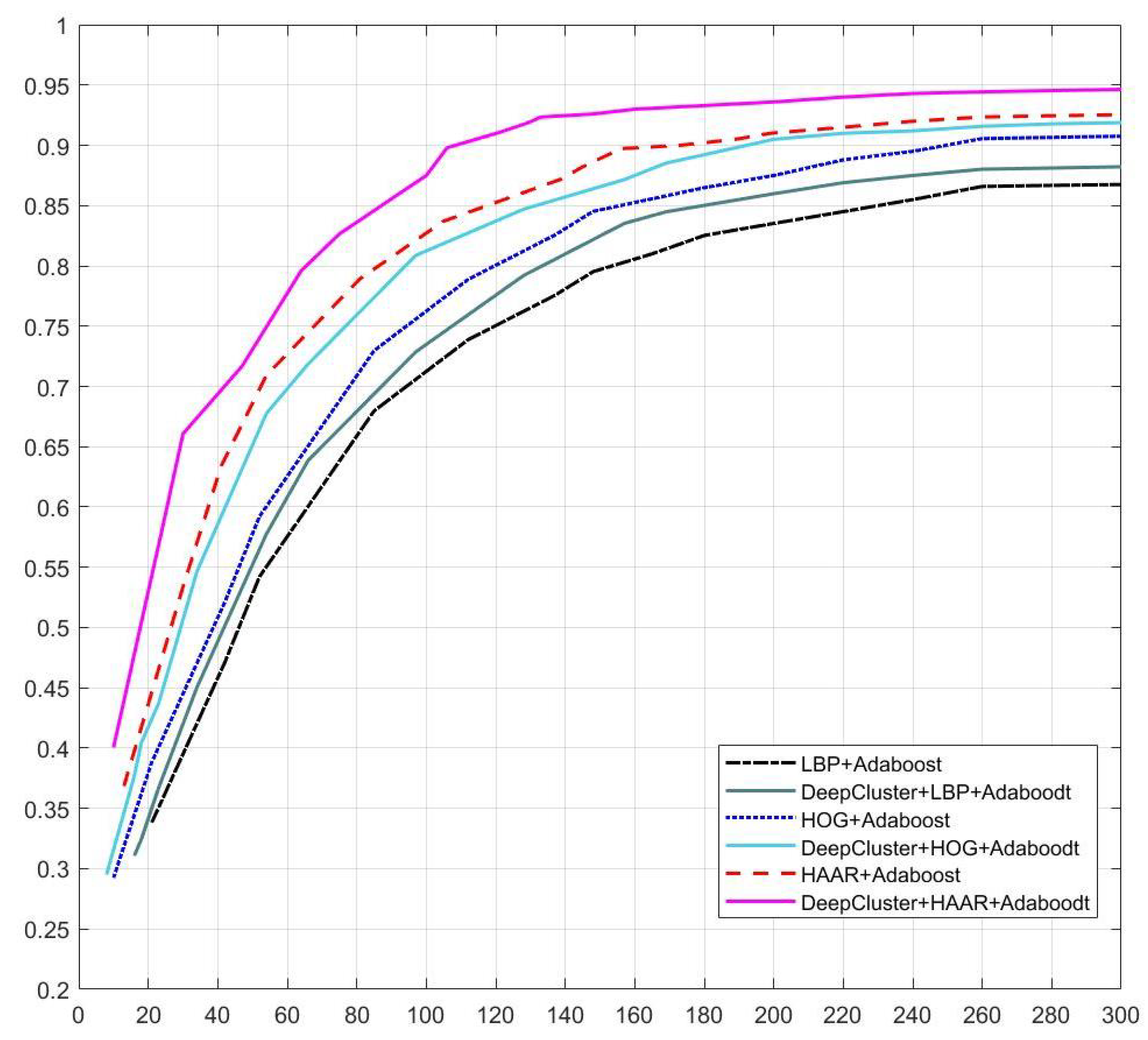
Figure 3 shows the ROC curves for the performance of the six modalities of the detector on the test dataset. To generate the ROC curves, we take the threshold of the last stage of the classifier from − to +, adjusting the different thresholds. Setting the threshold to +, all samples are determined to be non-vehicle and the detection rate and false detection rate are both 0. The previous method set the threshold to a very high value, but we take the threshold to a value greater than 10 with a detection rate of already 0. Adjusting the threshold to − will improve both the detection rate and the false detection rate. Since we are only adjusting the last stage, the previous classifier already has a certain detection performance, so both the detection rate and false detection rate will tend to a fixed value. The previous solution was to remove the last layer, but we found that when the threshold is taken above −10 it has already achieved the same effect as removing the last layer in the actual experiment. In order to construct complete ROC curves, we use the number of false positives on the x-axis of the ROC curves instead of the false positive rate to facilitate comparison with other systems.
The solution can be derived from Figure 3, compared with LBP and HOG features, the HAAR feature with the AdaBoost algorithm can better characterize the vehicle and detect the vehicle with the best results. We can also find that after introducing the framework of clustering, our algorithm has been dramatically improved compared with the original algorithm.
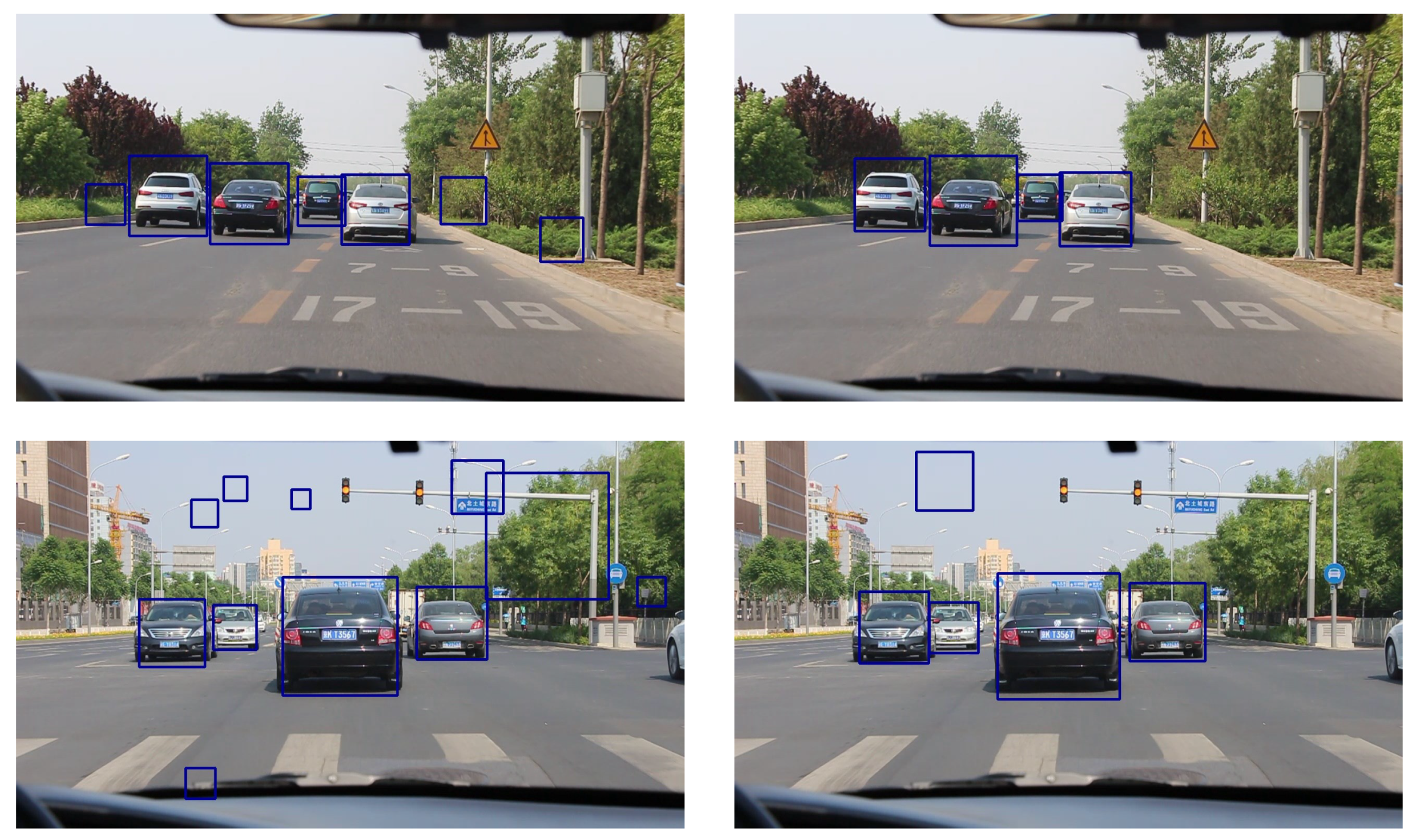
Table 3 shows the average time required to detect one frame of an image by the six approaches. Figure 4 displays the comparison of the detection effect of the two detectors.
From Table 3, we can conclude that the LBP feature combined with the AdaBoost algorithm is the fastest in detecting one frame and the HAAR feature is the slowest. We can conclude that the method we proposed improves a lot in the speed of the detection of vehicles. One of the main reasons responsible for this is that our algorithm excludes the road at the top level for traffic scenes with a heavy road share, so it speeds up the detection of one frame of an image.

4.3. Analysis of the Size of Dataset and Noise Resistance Performance

To better show the improvement in the performance of the vehicle detection using the algorithm we proposed, we add Gaussian noise to the image and observe the performance of vehicle detection under noisy conditions. Figure 3 shows the variation in the detection rate of the six algorithms with the addition of different noise conditions. It can be seen that after adding noise, our algorithm can increase the anti-interference performance of the original algorithm. Although both algorithms have significant false detection when the noise is relatively high, the anti-noise contribution of our algorithm to low-power noise cannot be denied. It is worth noting that we clustered the samples by the clustering algorithm and then trained them in a hierarchical manner, reducing the spacing within the samples and increasing the spacing between different samples. The features found in this way not only distinguish the vehicle from all other non-vehicle samples, but also for each class of samples, the features found can accurately distinguish them from the vehicle.
As illustrated clearly in Figure 5, the effect of the size of the dataset and the noise jamming on the accuracy of the algorithm are exhibited. The blue line is the traditional supervised learning algorithm, while the yellow line and the orange line are the unsupervised clustering algorithm we proposed. From the figure, we can clearly notice that the average time and the accuracy of the different algorithms remain essentially the same as the size of the dataset increases. It is apparent that our algorithm surpasses the traditional algorithm. Similarly, our algorithm still remains ahead, regardless of the increase in noise jamming. Moreover, although the accuracy of the algorithms decreases with increasing noise jamming, our algorithm decreases more slowly than the traditional one. In summary, the deep cascade AdaBoost with unsupervised clustering algorithms we proposed is superior to the traditional algorithm.

4.4. Sensitivity Analysis

The choice of parameters determines the performance of the algorithm in solving the evaluated optimization problem. We performed a sensitivity analysis [38] on the elements used in our model, such as the number of training stages, the size of training images, and false alarm rate. Sensitivity analysis was performed by using the One-at-a-Time (OAT) sensitivity measure [39], which is considered as one of the simplest strategies in sensitivity analysis. OAT examines the performance of the algorithm by varying a single parameter while keeping the other parameters constant. Table 4 and Table 5 describe in detail the changes in run time and TPR values for different parameter values whether or not DeepClustering is used. We used the HAAR feature as an example and chose ten different values within the interval of each parameter. Each variable underwent ten runs of the algorithm and the average values of run time and TPR are shown in the tables below.

5. Conclusions

In this paper, we propose an unsupervised clustering-based cascade-AdaBoost solution for vehicle detection. First, for an unknown scene, we applied unsupervised clustering on samples collected in the scene and assigned labels to the clustered samples as the training input of the AdaBoost algorithm. Then we proposed a hierarchical cascade-AdaBoost-based training approach and theoretically demonstrated the effectiveness of this approach in performing feature screening. We conducted experiments on HAAR, LBP, and HOG features separately. By comparing the three features cross-sectionally, we found that the HAAR feature is the best in detection accuracy. However, it takes the most time and features to train the model and also costs the most time to detect. LBP feature is fast, especially in terms of training time, but the detection accuracy is the worst. The performance of the HOG feature is generally between the other two features. Therefore, it is a compromise. We also compare the performance of the vehicle detector with the introduction of clustering longitudinally. The following conclusions can be obtained: compared with the traditional algorithm, the introduction of clustering not only improves the training process of the model but also shortens the training time and the number of stages of the model. In addition, the detection accuracy improves dramatically, witnessing considerable improvement in the detection rate and false detection rate. In brief, the method we proposed enhances the classification performance of vehicles and non-vehicles.

Author Contributions

Conceptualization, J.D.; methodology, J.D.; software, J.D.; validation, J.D., H.Y.; formal analysis, Z.L.; investigation, H.Y.; resources, Z.L.; data curation, H.Z.; writing—original draft preparation, J.D.; writing—Mreview and editing, H.Y. and J.D.; visualization, J.D.; supervision, Z.L.; project administration, H.Z. All authors have read and agreed to the published version of the manuscript.

Funding

This work was supported in part by the NSFC under Grant 61901341; in part by the China Postdoctoral Science Foundation under Grant 2021TQ0260 and Grant 2021M700105.

Data Availability Statement

Not applicable.

Conflicts of Interest

The authors declare no conflict of interest.

Abbreviations

The following abbreviations are used in this manuscript:
IoTInternet of things
NLPNatural language processing
CNNConvolutional neural network
HAARHaar-like features
HOGHistogram of oriented gradients
LBPLocal Binary Pattern
ROIRegion of Interest
TPRTure positive rate
FPRFalse positive rate

References

  1. Wang, L.; Ouyang, W.; Wang, X.; Lu, H. Visual Tracking with Fully Convolutional Networks. In Proceedings of the IEEE International Conference on Computer Vision, Las Vegas, NV, USA, 27–30 June 2016. [Google Scholar]
  2. Milan, A.; Rezatofighi, S.H.; Dick, A.; Schindler, K.; Reid, I. Online Multi-Target Tracking Using Recurrent Neural Networks. arXiv 2013, arXiv:1604.03635. [Google Scholar] [CrossRef]
  3. Ren, S.; He, K.; Girshick, R.B.; Sun, J. Faster R-CNN: Towards Real-Time Object Detection with Region Proposal Networks. CoRR 2015. Available online: https://doi.org/10.48550/arXiv.1506.01497 (accessed on 30 October 2022). [CrossRef] [PubMed] [Green Version]
  4. Girshick, R.B.; Donahue, J.; Darrell, T.; Malik, J. Rich feature hierarchies for accurate object detection and semantic segmentation. CoRR 2013. Available online: https://doi.org/10.48550/arXiv.1311.2524 (accessed on 30 October 2022).
  5. Lin, T.-Y.; Dollár, P.; Girshick, R.B.; He, K.; Hariharan, B.; Serge, J. Feature Pyramid Networks for Object Detection. CoRR 2016. Available online: https://doi.org/10.48550/arXiv.1612.03144 (accessed on 30 October 2022).
  6. Zhou, Z.; Zhao, X.; Wang, Y.; Wang, P.; Foroosh, H. CenterFormer: Center-based Transformer for 3D Object Detection. In European Conference on Computer Vision; Springer: Cham, Switzerland, 2022. [Google Scholar]
  7. Pavlitskaya, S.; Polley, N.; Weber, M.; Zöllner, J.M. Adversarial Vulnerability of Temporal Feature Networks for Object Detection. arXiv 2022, arXiv:2208.10773. [Google Scholar] [CrossRef]
  8. Ham, J.; Chen, Y.; Crawford, M.M.; Ghosh, J. Investigation of the random forest framework for classification of hyperspectral data. IEEE Trans. Geosci. Remote. Sens. 2005, 43, 492–501. [Google Scholar] [CrossRef] [Green Version]
  9. Antonio, B.; Davide, M.; Massimo, M. Efficient Adaptive Ensembling for Image Classification. arXiv 2022, arXiv:2206.07394. [Google Scholar] [CrossRef]
  10. Schuldt, C.; Laptev, I.; Caputo, B. Recognizing human actions: A local SVM approach. In Proceedings of the International Conference on Pattern Recognition, Cambridge, UK, 26 August 2004. [Google Scholar]
  11. Dasom, A.; Sangwon, K.; Hyunsu, H.; Byoung, C.K. STAR-Transformer: A Spatio-temporal Cross Attention Transformer for Human Action Recognition. arXiv 2022, arXiv:2210.07503. [Google Scholar] [CrossRef]
  12. Viola, P.A.; Jones, M.J. Rapid Object Detection using a Boosted Cascade of Simple Features. In Proceedings of the Computer Vision and Pattern Recognition, CVPR, Kauai, HI, USA, 8–14 December 2001. [Google Scholar]
  13. Islam, M.T.; Ahmed, T.; Raihanur Rashid, A.B.M.; Islam, T.; Rahman, S.; Habib, T. Convolutional Neural Network Based Partial Face Detection. In Proceedings of the 2022 IEEE 7th International conference for Convergence in Technology (I2CT), Mumbai, India, 7–9 April 2022. [Google Scholar]
  14. Ojala, T.; Pietikainen, M.; Maenpaa, T. Multiresolution Gray-Scale and Rotation Invariant Texture Classification with Local Binary Patterns. IEEE Trans. Pattern Anal. Mach. Intell. 2002, 24, 971–987. [Google Scholar] [CrossRef]
  15. Arreola, L.; Gudiño, G.; Flores, G. Object Recognition and Tracking Using Haar-Like Features Cascade Classifiers: Application to a Quad-Rotor UAV. arXiv 2019, arXiv:1903.03947. [Google Scholar]
  16. Dalal, N.; Triggs, B. Histograms of Oriented Gradients for Human Detection. In Proceedings of the IEEE Computer Society Conference on Computer Vision Pattern Recognition, San Diego, CA, USA, 20–25 June 2005. [Google Scholar]
  17. Kitayama, M.; Kiya, H. Generation of Gradient-Preserving Images allowing HOG Feature Extraction. In Proceedings of the 2021 IEEE International Conference on Consumer Electronics-Taiwan (ICCE-TW), Penghu, Taiwan, 15–17 September 2021. [Google Scholar]
  18. Alhindi, T.J.; Kalra, S.; Ng, K.H.; Afrin, A.; Tizhoosh, H.R. Comparing LBP, HOG and Deep Features for Classification of Histopathology Images. In Proceedings of the 2018 International Joint Conference on Neural Networks (IJCNN), Rio de Janeiro, Brazil, 8–13 July 2018. [Google Scholar]
  19. Abdelhamid, A.A.; El-Kenawy, E.-S.M.; Khodadadi, N.; Mirjalili, S.; Khafaga, D.S.; Alharbi, A.H.; Ibrahim, A.; Eid, M.M.; Saber, M. Classification of Monkeypox Images Based on Transfer Learning and the Al-Biruni Earth Radius Optimization Algorithm. Mathematics 2022, 10, 3614. [Google Scholar] [CrossRef]
  20. Hui, Y.; Cheng, N.; Su, Z.; Huang, Y.; Zhao, P.; Luan, T.H.; Li, C. Secure and Personalized Edge Computing Services in 6G Heterogeneous Vehicular Networks. IEEE Internet Things J. 2022, 9, 5920–5931. [Google Scholar] [CrossRef]
  21. Hui, Y.; Su, Z.; Tom, H. Luan: Unmanned Era. A Service Response Framework in Smart City. IEEE Trans. Intell. Transp. Syst. 2022, 23, 5791–5805. [Google Scholar] [CrossRef]
  22. Schmidhuber, J. Deep Learning in Neural Networks: An Overview. Neural Netw. 2015, 61, 85–117. [Google Scholar] [CrossRef] [PubMed] [Green Version]
  23. Xie, J.; Girshick, R.; Farhadi, A. Unsupervised Deep Embedding for Clustering Analysis. Comput. Sci. 2015. Available online: https://doi.org/10.48550/arXiv.1511.06335 (accessed on 30 October 2022). [CrossRef]
  24. Mong, Y.-L.; Ackley, K.; Killestein, T.L.; Galloway, D.K.; Vassallo, C.; Dyer, M.; Cutter, R.; Brown, M.J.I.; Lyman, J.; Ulaczyk, K.; et al. Self-Supervised Clustering on Image-Subtracted Data with Deep-Embedded Self-Organizing Map. Mon. Not. R. Astron. Soc. 2022, 518, 152–762. [Google Scholar] [CrossRef]
  25. Yang, J.; Parikh, D.; Batra, D. Joint Unsupervised Learning of Deep Representations and Image Clusters. In Proceedings of the IEEE Conference on Computer Vision and Pattern Recognition, Las Vegas, NV, USA, 27–30 June 2016; pp. 5147–5156. [Google Scholar]
  26. Chang, J.; Wang, L.; Meng, G.; Xiang, S.; Pan, C. Deep Adaptive Image Clustering. In Proceedings of the 2017 IEEE International Conference on Computer Vision (ICCV), Venice, Italy, 22–29 October 2017. [Google Scholar]
  27. Quinlan, J.R. Induction of decision trees. Mach. Learn. 1986, 1, 81–106. [Google Scholar] [CrossRef] [Green Version]
  28. Quinlan, J. Program for Machine Learning; C4.5 Morgan Kaufmann Publisher: San Mateo, CA, USA, 1993. [Google Scholar]
  29. Nasraoui, O. Web Data Mining: Exploring Hyperlinks, Contents, and Usage Data. Acm Sigkdd Explor. Newsl. 2008, 10, 23–25. [Google Scholar] [CrossRef]
  30. Caglar, A. Neural Networks Are Decision Trees. arXiv 2022, arXiv:2210.05189. [Google Scholar] [CrossRef]
  31. Louppe, G. Understanding Random Forests: From Theory to Practice. arXiv 2014, arXiv:1407.7502. [Google Scholar]
  32. Breiman, L. Random Forests–Random Features. Mach. Learn. 2001, 45, 5–32. Available online: https://link.springer.com/article/10.1023/a:1010933404324 (accessed on 11 October 2022).
  33. Dempster, A. Maximum-likelihood from incomplete data via the EM algorithm. J. R. Stat. Soc. 1977, 39, 1–22. [Google Scholar]
  34. Mclachlan, G.J.; Krishnan, T. The EM Algorithm and Extensions: Second Edition; John Wiley & Sons: Hoboken, NJ, USA, 2007. [Google Scholar]
  35. Freund, Y.; Schapire, R.E. Schapire (translation by Naoki Abe). A short introduction to boosting. Artif. Intell. 1999, 14, 771–780. (In Japanese) [Google Scholar]
  36. Hastie, T.; Tibshirani, R.; Friedman, J. The elements of statistical learning, 2001. J. R. Stat. Soc. 2004, 167, 192. [Google Scholar]
  37. Caron, M.; Bojanowski, P.; Joulin, A.; Douze, M. Deep Clustering for Unsupervised Learning of Visual Features. CoRR 2018. Available online: https://doi.org/10.48550/arXiv.1807.05520 (accessed on 30 October 2022).
  38. El-kenawy, E.-S.M.; Albalawi, F.; Ward, S.A.; Ghoneim, S.S.M.; Eid, M.M.; Abdelhamid, A.A.; Bailek, N.; Ibrahim, A. Feature Selection and Classification of Transformer Faults Based on Novel Meta-Heuristic Algorithm. Mathematics 2022, 10, 3144. [Google Scholar] [CrossRef]
  39. Confalonieri, R.; Bellocchi, G.; Bregaglio, S.; Donatelli, M.; Acutis, M. Comparison of sensitivity analysis techniques: A case study with the rice model WARM. Ecol. Model. 2010, 221, 1897–1906. [Google Scholar] [CrossRef]
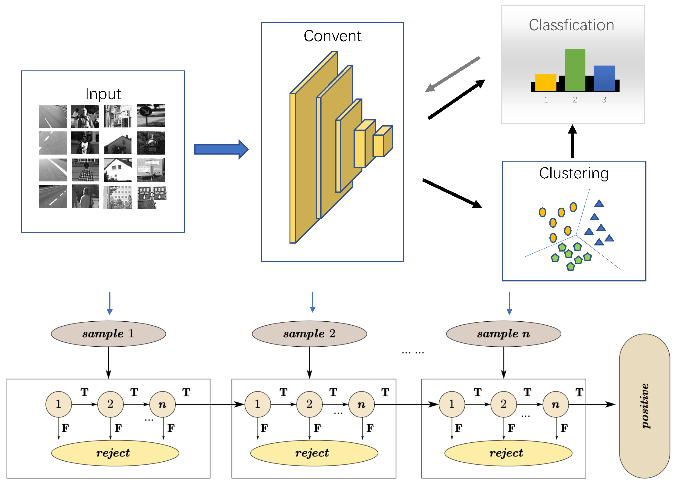
Figure 1. The convolutional neural network is used as the feature extractor, the unsupervised clustering algorithm is used to cluster the samples, and then the Cascade AdaBoost method is used for training according to the sequence. Finally, the object detection model is generated.
Electronics 12 00044 g001
Figure 2. Examples of a figure caption.
Electronics 12 00044 g002
Figure 3. ROC curves for the performance of the six modalities of the detector on the test dataset.
Electronics 12 00044 g003
Figure 4. Comparison of the detection effect of the two detectors.
Electronics 12 00044 g004
Figure 5. The effect of the size of the dataset and noise jamming on the accuracy of the algorithm.
Electronics 12 00044 g005
Table 1. Train of six vehicle detection methods.
MethodTime Cost (h)Number of FeaturesNumber of Training Stages
HAAR + AdaBoost57 ± 0.563530
LBP + AdaBoost12 ± 0.530220
HOG + AdaBoost33 ± 0.547725
DeepCluster + HAAR + AdaBoost23 ± 0.553826
DeepCluster + LBP + AdaBoost9 ± 0.518716
DeepCluster + HOG + AdaBoost20 ± 0.541222
Table 2. Evaluation results of six vehicle detection methods.
MethodTPRFPR
HAAR + AdaBoost91.88%6.83%
LBP + AdaBoost86.75%12.73%
HOG + AdaBoost90.76%9.66%
DeepCluster + HAAR + AdaBoost94.40%3.59%
DeepCluster + LBP + AdaBoost88.22%10.49%
DeepCluster + HOG + AdaBoost92.55%7.31%
Table 3. Time for six vehicle detectors to detect one image frame.
MethodDetection Time (ms)
HAAR + AdaBoost42
LBP + AdaBoost26
HOG + AdaBoost33
DeepCluster + HAAR + AdaBoost36
DeepCluster + LBP + AdaBoost24
DeepCluster + HOG + AdaBoost28
Table 4. Sensitivity analysis results using HAAR + AdaBoost.
Number of Training StagesSize of Training ImagesFalse Alarm Rate
ValuesRun TimeTPRValuesRun TimeTPRValuesRun TimeTPR
2040.9680.12%2041.7290.27%0.0541.9291.88%
2141.8382.71%2142.3390.93%0.1042.3491.77%
2242.9183.90%2241.9691.24%0.1541.0491.54%
2343.0185.24%2342.2291.36%0.2042.8590.93%
2445.2087.93%2442.1791.88%0.2542.1590.77%
2546.3689.90%2542.1291.96%0.3042.1889.64%
2648.2290.24%2642.1391.99%0.3542.4487.53%
2745.1390.89%2742.0992.03%0.4042.0785.15%
2844.7891.20%2842.1191.89%0.4543.7182.38%
2943.1791.77%2942.1091.77%0.5044.2179.94%
3042.1091.88%3042.1091.86%0.5544.7977.42%
Table 5. Sensitivity analysis results using DeepCluster + HAAR + AdaBoost.
Number of Training StagesSize of Training ImagesFalse Alarm Rate
ValuesRun TimeTPRValuesRun TimeTPRValuesRun TimeTPR
2034.8185.68%2035.5594.16%0.0535.9394.90%
2135.6887.59%2136.1694.82%0.1036.5494.67%
2236.7688.95%2235.7995.13%0.1535.9294.44%
2337.8689.80%2336.0595.62%0.2036.2593.81%
2439.0590.07%2435.9795.85%0.2536.1693.48%
2540.2191.33%2535.9595.87%0.3036.4492.61%
2640.0792.75%2635.9695.89%0.3536.8590.55%
2738.1893.32%2735.9295.93%0.4037.1187.22%
2837.6393.79%2835.9495.88%0.4537.6485.56%
2936.3294.43%2935.9395.95%0.5038.1383.49%
3035.9594.90%3035.9395.89%0.5538.4982.90%
Disclaimer/Publisher’s Note: The statements, opinions and data contained in all publications are solely those of the individual author(s) and contributor(s) and not of MDPI and/or the editor(s). MDPI and/or the editor(s) disclaim responsibility for any injury to people or property resulting from any ideas, methods, instructions or products referred to in the content.